Developing advanced x-ray scattering methods combined with crystallography and computation

Abstract

The extensive use of small angle x-ray scattering (SAXS) over the last few years is rapidly providing new insights into protein interactions, complex formation and conformational states in solution. This SAXS methodology allows for detailed biophysical quantification of samples of interest. Initial analyses provide a judgment of sample quality, revealing the potential presence of aggregation, the overall extent of folding or disorder, the radius of gyration, maximum particle dimensions and oligomerization state. Structural characterizations include ab initio approaches from SAXS data alone, and when combined with previously determined crystal/NMR, atomistic modeling can further enhance structural solutions and assess validity. This combination can provide definitions of architectures, spatial organizations of protein domains within a complex, including those not determined by crystallography or NMR, as well as defining key conformational states of a protein interaction. SAXS is not generally constrained by macromolecule size, and the rapid collection of data in a 96-well plate format provides methods to screen sample conditions. This includes screening for co-factors, substrates, differing protein or nucleotide partners or small molecule inhibitors, to more fully characterize the variations within assembly states and key conformational changes. Such analyses may be useful for screening constructs and conditions to determine those most likely to promote crystal growth of a complex under study. Moreover, these high throughput structural determinations can be leveraged to define how polymorphisms affect assembly formations and activities. This is in addition to potentially providing architectural characterizations of complexes and interactions for systems biology-based research, and distinctions in assemblies and interactions in comparative genomics. Thus, SAXS combined with crystallography/NMR and computation provides a unique set of tools that should be considered as being part of one’s repertoire of biophysical analyses, when conducting characterizations of protein and other macromolecular interactions.

1.1 Introduction

The importance of studying protein interactions to gain a coherent understanding of complex biological systems has been highlighted by the plethora of tools that have been created to analyze such interactions. This is because the progression of cellular pathways, and often catalysis, is largely controlled through such interactions. Tools critical to defining these interactions may characterize proteins at atomic resolution or function at the level of studying the entire interactomics system of a cell. At higher-resolution, detailed crystallographic, nuclear magnetic resonance (NMR) and electron microscopy (EM) studies have revealed profound insights into the molecular mechanisms of cellular machines functioning to control fundamental biological processes. Examples include analyses of the molecular machines involved in the many different DNA metabolism steps of DNA replication, recombination or repair [1, 2]. These studies have often been supported by biophysical techniques providing values to binding affinities, on-off rates of protein interactions and complex formations, and helping to identify allosteric control mechanisms. Yet, much still remains to be defined due to the inherent difficulties in studying large, complex molecular machines and their interactions, and the inherent limitations of the structural methods being used.

One technique whose beginnings date back to the 1930s, and is now very much coming to the fore for studying protein interactions, is in-solution small angle x-ray scattering (SAXS). The interest being generated in this powerful, complimentary and robust technique is that there is a lack of size constraints that can hinder other methods such as NMR or EM. Also, there is no requirement for diffraction-quality crystals as needed for macromolecular crystallography. Disadvantages of SAXS are that rotational averaging of the data means that enantiomorphs cannot be distinguished, and that the structural models produced contain lower information content akin to low-resolution EM images, with data in the 10–30 Å range. Importantly however, SAXS has very rapid data collection and processing times relative to other structural techniques. Also, SAXS analyses are conducted in solution that can include near physiological conditions including ambient temperatures, and with minimal sample preparation. Thus, SAXS readily lends itself to charactering protein interactions, flexibility, conformational changes and formations or disruptions of higher order complexes, and has an added advantage of being a higher throughput method than the other major structural techniques.

The ability of SAXS to characterize flexibility in larger proteins and complexes is a noticeable asset when studying protein interactions [3]. Interestingly, eukaryotic proteins contain significant regions of flexibility and disorder [4], more than typically observed proteins in bacteria or archaea [5, 6]. The increased flexibility likely reflects more complex regulatory roles for eukaryotic proteins. This could be through the occurrence of post-translational modifications within the regions of disorder that are more accessible by the modification machinery, and through conformational controls and switches regulating enzymatic activities or pathway progression through protein partner handoffs. However, in crystallography these disordered regions are often removed to aid crystallization or are not clearly visible in the electron density maps unless they are involved in a crystal-packing interface. Moreover, certain flexible regions are known to have disorder-to-order transitions, upon partner interactions that can promote catalytic activities or cellular signaling. SAXS studies can reveal these key switches within global architectures in solution, albeit at lower resolution. Additionally, SAXS is a very sensitive technique for defining assemblies, including transient complexes, as the scattering power in SAXS is related to the square of the number of electrons in the protein/complex, and as such, the formation of larger complexes can be readily observed. These mixtures of the individual proteins and their higher order assemblies can be deconvoluted, providing that the initial protein constituents are known.

Combining high-resolution information from crystallography or NMR to SAXS data generates an effective hybrid method to reveal key biological insights into protein interactions. This combinatorial approach has been aided and developed in recent years through the advances in computing power and new SAXS algorithms and software to provide detailed analyses, and due to the ease of sample preparation and speed of data collection. As an example, it can be difficult to identify the correct biological oligomer within a crystal from crystal packing interfaces alone, but SAXS analyses can define the in solution biological oligomer and hence reveal the best match within the crystal (e.g. [7, 8]). Similarly, SAXS data can distinguish cases in which the solution behavior of a sample does not perfectly match the crystalline assembly, perhaps due to conformational relaxation from forced crystal contacts. Another application is to study larger, inherently flexible molecules, which high-resolution techniques have difficulties in analyzing due to being out of the typical range of NMR or being a notable challenge to crystallize. Here, SAXS analyses can reveal holo-architectures that can be fitted with individual domains that have been determined by NMR and/or crystallography. Advantageously, the use of 96-well plate technology and data collection time of seconds, allows for hundreds of samples to be analyzed within a typical allocation of 8-hrs beamtime, enabling the holo-architectures to be characterized in detail. This includes defining interactions with multiple partners, substrates, co-factors, altering buffer conditions etc, to define overall architectural structural states.

Here, we highlight these recent developments in SAXS for studying protein interactions, provide methods and examples of results used to gain such information on flexible and reversible molecular complexes. In particular, we discuss applications and provide our insights that have been gained from SAXS studies from our own research and that of collaborators, which have been conducted at the Structurally Integrated BiologY for Life Sciences (SIBYLS) beamline, Advanced Light Source (ALS), Berkeley National Laboratory, Berkeley, California. Despite the growth of SAXS studies that are markedly helping define key biomolecular complexes and interactions, these methods are under-utilized and underexplored. For example, SAXS could be utilized as a tool in the early states of drug discovery. Here, much of the low-hanging fruit in drug discovery has been plucked, leaving more challenging structural-targets, requiring new approaches characterizing protein interactions and assemblies, and disrupting or stabilizing these via small molecules. SAXS clearly falls within this this category, being of potential benefit due to an ability to both screen and produce structure and conformation-based outputs rapidly and facilely. Thus, through this review we hope to provide the reader with an understanding of the latest methods and practical uses of SAXS, encouraging those interested to explore and further evolve the uses SAXS methods to define protein interactions to uncover new insights into biological processes.

1.2 Methods

In addition to home sources, SAXS data is routinely collected at multiple synchrotron beamlines across the world, with a list of current SAXS capable beamlines at Wikipedia (http://en.wikipedia.org/wiki/Small-angle_X-ray_scattering). Our data is collected at the ‘Structurally Integrated Biology for Life Sciences’ (SIBYLS) beamline 12.3.1 at the ALS. A user can request SIBYLS SAXS time by visiting the RAPIDD access link on the SIBYLS beamline homepage at http://bl1231.als.lbl.gov. SIBYLS is a dual function end station for SAXS (schematic of SAXS setup depicted in Fig. 1) and crystallography. Switching between the SAXS and crystallographic data collection modes takes approximately 1 hr, enabling a user to collect both SAXS and crystallographic data on a single visit to the beamline. Data is generally collected on 15–25 μl sample volumes at 1–5 mg/ml range, with at least 3 serial dilutions preferred. Data is collected in the order of buffer, lowest concentration, medium concentration(s) and highest concentration, and lastly a second buffer is measured. The sample cell is washed both between the highest-concentration sample and subsequent second buffer, as well as between differing protein samples by a mild detergent for 1 min, followed by 3 rinses in buffer solution. The data collection occurs in a high-throughput fashion, using a 96-well plate and pipetting robot that loads samples into the sample cell, which is situated in a positive helium pressure to reduce air scatter and oxidative damage [9]. The sample plate is typically maintained at 15 °C prior to chamber dispensing, and temperature can be altered for increased user-control. Control software for this high throughput data collection has been developed from the Blu-Ice/DCS control systems, which is used from crystallography data collection at certain synchrotron beamlines [10].

Fig. 1.

Schematic of the SAXS end station at the SIBYLS 12.3.1 beamline, ALS.

Data for each sample is typically collected by four exposures of 0.5, 1, 2 and 4 secs, although longer exposures, such as up to 40 secs, are collected if there is an interest collecting at the highest resolutions. The scattering profiles of the buffers collected before and after the molecule samples are compared, to ensure to no significant errors have occurred from the instrumentation or from bubbles occurring from loading the buffer blank. Similarly, a photographic image of the sample cell captured for each sample ensures proper loading and lack of bubbles.

In addition to on-site data collection, this high-throughput setup allows for mail-in format, where the user ships to the technical staff their 96-well PCR microplate (Axygen Scientific, catalog no. PCR-96-FS-C) containing samples and which is sealed by a silicon mat (Axygen Scientific, catalog no. AM-96-PCR-RD). If shipped frozen, the plate is subsequently thawed and spun, before it is used for data collection with the aid of the pipetting robot that adds and removes samples to the sample cell. The data output is then mailed to the user, with annotated comments on global data collection success. The instrumentation is set up so that the beam at the sample cell has a relatively large spread, in an effort to minimize radiation damage, and is narrowly focused at the detector, allowing for a relatively small beamstop. Usually x-rays at ~1 Å wavelength are used, providing significant flux of 10¹² photons s⁻¹, although longer wavelengths can be used allow for data collection on samples with dimensions significantly greater than the norm.

1.3 Results

1.3.1. Generating the SAXS Profile

Here, we focus on key methods for SAXS analyses and describe recent developments that combined crystallography and computation with SAXS analyses for studying protein complexes. For a detailed background on SAXS theory, we refer the readers to elegant reviews [11–13]. We also refer the readers to a detailed review that provides a comparison between protein crystallography and SAXS theory and techniques, and also provides comparisons of SAXS software programs [14]. In SAXS, the signal difference between the sample and buffer is small (although the contrast will vary for different macromolecules and buffer conditions), and thus the buffer data is subtracted from the sample measurement, which at SIBYLS is through a script that can be automated for high throughput studies [9]. This background subtraction generates the scattering profile of the macromolecule, which plots intensity, I, in detector units versus distance (q) A⁻¹. (Fig. 2). Often the y-axis is I(q) to provide a wavelength- and detector-independent scattering profile, where q is the photon momentum transfer, and q = 4πsin(θ)/λ, with 2θ being the scattering angle relative to the incident beam and λ the wavelength. The buffer subtraction step also helps to remove background scattering from the data, which can occur from the primary beam and could otherwise add significant noise. The generated SAXS profile represents both the size and shape of the macromolecule, present in all possible orientations in solution (2). Importantly, for subsequent analyses, no two unique structures produce the same scattering profile [15, 16], although low-resolution data may prove very similar. For this reason, the current q-range for our MarCCD 165 detector is typically 0.01–0.32 Å to ensure finer resolution features can be distinguished from the SAXS experiment.

Fig. 2.

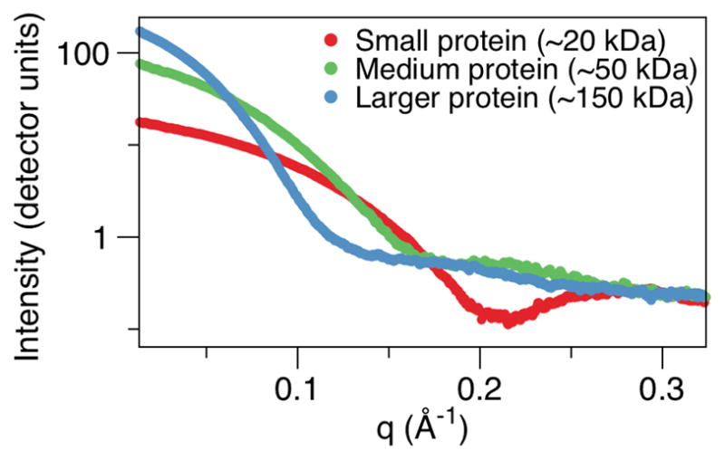
The unique scattering profiles of the 3 different sized macromolecules (unpublished experimental data) with the scattering profile being intensity, I, plotted against the photon momentum transfer, q.

The ATSAS software suite [17], as developed by the Svergun laboratory (http//www.embl-hamburg.de/biosaxs/software.hmtl), is typically used for initial analysis of SAXS data, in addition to its uses in later shape reconstructions. The ATSAS software component PRIMUS [18], is used to plot the buffer-corrected scattering data generated, in addition to generating a number of subsequent plots. These plots are used to define several parameters, including the maximum particle dimension, d_max, radius of gyration, R_G, volume and provide a mass estimation and hence the oligomerization state. This is in addition to a qualitative measure of the presence of aggregation, flexibility and disorder.

Radiation damage can induce aggregation or complex disassociations, as observed by a change in the intensity at close to zero scattering angle, I(0) (Figs. 3,5). An initial comparison of two scattering curves of the same sample shot before and after a long-exposure shot allows for the identification of any such potential radiation sensitivity. If inherent radiation sensitivity is observed, measures to deal with this include adding free radical scavengers and/or protectants such as glycerol to the sample buffer, or cooling and/or diluting the sample. This is important, as radiation-induced changes adversely affect data analyses [19], often precluding further modeling. Next, a scaled comparison of the scattering profiles of the sample at different concentrations is conducted to identify any potential concentration dependent interactions, which would alter the signal at the lowest q ranges and can adversely affect the analyses. If observed, using alternate buffer conditions and/or increasing the salt concentration may ameliorate these long-ranged interactions. However, the current, less than ideal data may still be analyzed, through an extrapolation of this data to a zero concentration point. A final, merged scattering curve for the sample at a specific concentration with improved signal-to-noise, is generated through merging the short, medium and long exposures, and removing parts of these that do not readily superimpose, which is often the higher q range in shorter exposures.

Fig. 3.

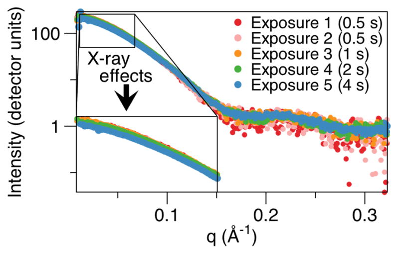
Radiation damage from increasing x-ray exposure induces the disassociation of a protein complex being analyzed (unpublished experimental data) as observed by a decrease in the scattering intensities close to zero scattering angle.

Fig. 5.

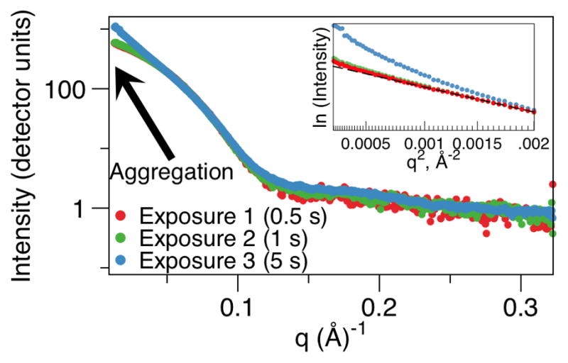
Radiation damage induces aggregation within a sample being analyzed by SAXS (unpublished experimental data). The intensity close to I(0) increases, and the slope of the Guinier region shown by the insert loses its linearity at the longest exposure.

1.3.2. Estimating maximum particle dimension, radius of gyration and molecular weight

X-ray scattering from proteins is a function of their electron density, where a Fourier transformation of the SAXS curve gives an electron pair distribution function, P(r), of the interatomic vectors within the biomolecule, which is a plotted against real space radius, r in Å, where:

$$\text{I}(q)=4\pi \underset{\text{o}}{\overset{d_{max}}{\int }}\text{P}(\text{r})\frac{sin(q\text{r})}{q\text{r}}\text{dr}$$

Thus, the P(r) distribution can be used to estimate the maximum dimension of the molecule, d_max, a parameter used in later shape reconstructions. Gross features can be gained from this plot, as a globular molecule will have a single P(r) peak, a bilobal molecule giving two, while an elongated conformation in solution will have an extended, skewed plot that gives a relatively large d_max. This P(r) distribution is particularly useful in sample comparisons, such as changes in oligomerization state (Fig. 4), which will result in changes in the shape of the P(r) curve and the d_max value. Conformational switching or changes in flexibility may also be revealed by changes in the shape of the P(r) curve and d_max value.

Fig. 4.

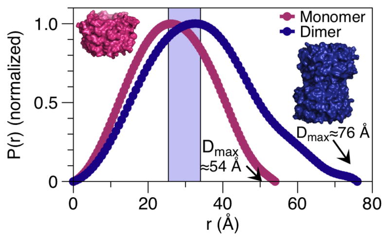
Changes in oligomerization state, as observed by alteration of the P(r) distribution and d_max value, which is where the curve intercepts the x-axis.

The radius of gyration, R_G, is a value that defines the mass distribution of the molecule about its center of gravity, and can be estimated from the P(r) function, such as provided by the GNOM program run within PRIMUS, through an integration of the function with r² over all values of r:

$${{\text{R}}_{\text{G}}}^2=\underset{\text{o}}{\overset{d_{max}}{\int }}{\text{r}}^2\text{P}(\text{r})\text{dr}/\underset{\text{o}}{\overset{d_{max}}{\int }}\text{P}(\text{r})\text{dr}$$

The R_G value can also be estimated from the slope of the plot of ln[I(q)] versus q² in the Guinier region, in addition to an estimated intensity at zero scattering angle I(0) at the y-axis intercept. The Guinier approximation, I(q) = I(0) exp[−(q²R_G²/3)], describes the scattering of a particle, and remains valid at lower resolutions such that data is examined at q.R_G < 1.3 for globular proteins. Disagreements in the ‘real space’ R_G, as calculated from the P(r) of function and that calculated in reciprocal space by the Guinier plot are suggestive of small amounts of aggregation that will primarily affect the low resolution Guinier range. Aggregation can arise after purification steps, could have occurred at later stages such as freeze-thawing of the samples or be induced by radiation damage during data collection (Fig. 5). The Guinier plot will indicate the presence of aggregation through the slope in the Guinier region not being linear, while at the same time the P(r) function will indicate an extended conformation with a difficult-to-determine d_max. This is observed, further analyses should be taken with extreme care, as the aggregated sample is likely to greatly affect the data, such as by overestimating d_max. One common method for removing suspected aggregates before data collection is a gel filtration purification step at the beamline, followed by immediate data collection on the fractions. A second, relatively quick method is passing the sample through a large molecule weight spin filter, where the filtrate contains the non-aggregated components that are used for the subsequent data collection. However, appropriate methods to ensure a lack of aggregation should ideally be conducted prior to SAXS analyses (e.g. analytical gel filtration, ideally coupled to static and/or dynamic light scattering). Methods to inhibit radiation induced aggregation, as revealed by samples having increasing R_G and I(0) with increasing exposure, include shooting samples in an appropriate buffer that includes 5% glycerol. Once the possibility of aggregation has been eliminated, the opening or closing of the molecule/complex, such as observed when adding a ligand that induces a conformational change, can be observed through changes in this R_G value.

A number of methods can be used and compared for an estimation of molecular mass, and hence multimeric state. One common means is to generate a calibration curve of data collected with control samples of known mass, such as lysozyme, bovine serum albumin, etc, in the same buffer as that in the sample being measured. From this a linear plot of molecular weight versus I(0)/concentration can be created, from which the molecular weight of the sample can be estimated [20]. Care, however, should be taken with control samples, which should be representative of the sample (i.e. similar shape and density), as for example, nucleotide:protein complexes may not be so accurately measured against protein only controls. Quicker approaches to estimating molecular mass include a rough estimate of mass from the Porod volume as estimated within the P(r) plotting function in PRIMUS x 1.2/2. Not surprisingly, proteins away from the norm in shape and size have less of an agreement to this approximation. Also, a useful molecular weight estimation tool on the web is SAXS MoW (http://www.if.sc.usp.br/~saxs/saxsmow.html) that estimates molecular mass through a calculation of volume times the average protein density of 0.83 × 10⁻³ kDa A⁻³ [21].

1.3.3. Defining a folded versus unfolded state

The Kratky plot (q²I(q) versus q), is used to provide estimation of whether the macromolecule is folded, has partial disorder or is unfolded. A folded sample obeys Porod’s law, resulting in a parabolic shape with the position of the peak roughly correlated to the size of the complex [22]. However, when the sample is unstructured the plot does not diminish after the peak, and has a hyperbolic shape. In a macromolecule exhibiting partial disorder, such as a protein domain with flexible N- and/or C-terminal region, the initial peak is parabolic, but forms a higher baseline with increasing q. Here, care should be taken in using an exact buffer blank, as inaccurate buffer blank subtraction can also result in increased baseline, especially at the higher q regions. An appropriate blank is typically created by dialysis, gel filtration or spin-concentrator buffer exchange, and not by simply attempting to mimic or recreate the sample buffer. Another, perhaps underutilized approach in SAXS to detecting flexibility is the use of the Porod-Debye law [23]. Interestingly, the Porod plot of q⁴I(q) versus q, as plotted in PRIMUS, may be more effective than the Kratky plot to differentiate between a macromolecule that has a change in conformation, versus a macromolecule that has a localized change in flexibility. In the low range of data, akin to the Guiner plot, the plot of an ordered protein will contain an increasing value that plateaus. If a ligand is added that induces a distinct conformational change, plotting of this second set of data will reveal a plateau in the low q range, but if ligand binding results in a increase in flexibility, the plateau is lost. As such, in our studies on the Mre11-Rad50 DNA repair complex, analysis of the Kratky plot suggested that in the presence and absence of ATP, this repair complex changes between two conformational states. However, upon closer analysis, the Porod plots instead suggested that the complex was in a compact shape in the presence of ATP and become more flexible in its absence [23, 24] (Fig. 6).

Fig. 6.

SAXS analysis of the Mre11-Rad50 DNA repair complex, in the presence and absence of ATP. A) The SAXS profile combined with the Kratky plots, upper right panel, indicated a change between two conformational states in the presence of ATP (black line) or the absence of ATP (red line). B) The Porod plots more clearly define that the complex is in a compact shape in the presence of ATP (black line), and becomes more flexible in its absence (red line). Figure adapted from experimental data [23, 24].

1.3.4. SAXS Structural databases

The scattering curve of a macromolecule of interest can be compared to those pre-calculated from structures deposited in the protein databank (PDB). This enables finding structural neighbors, by an approach distinct from classical sequence search based methods. The DARA database contains scattering profiles for a large fraction of deposited structures in the PDB, with some homologous structures removed [15, 16]. The relative fit of the experimental profile is compared to these pre-calculated scattering profiles, where close scoring hits have in general a similar overall shape and fold to the macromolecule of interest. Difficulties in this approach can arise when the biological assembly is not correctly defined, or when residues with multiple conformations or containing heavy atoms for phasing are included in the PDB file [25]. This SAXS structural homology search has a number of interesting uses. This includes identifying homologues to be used for molecular replacement searches for phasing in crystallography, or for high-throughput studies [9, 26], such as those focusing on proteome analyses or structural and comparative genomics. A second SAXS structural database has also been developed, BIOISIS (http://www.bioisis.net). The function of BIOISIS is to be an open access database for the deposition, distribution and maintenance of small angle X-ray scattering data. The deposited data includes the initial scatting curve, P(r), Guinier, and Kratky plots, in addition to the protein and/or nucleotide sequence of the macromolecule, and the final structural model(s) and methods used for modeling.

1.3.5. Ab initio structural modeling

Shape reconstructions can proceed if the initial SAXS analyses determine that the sample is monodisperse, does not suffer from significant radiation damage and does not have long-range concentration-dependent interactions. Generation of macromolecular models from the SAXS data is by either ab initio, rigid body modeling methods or by a combination of these [14]. If the researcher lacks an input atomic structure, ab initio methods can be used to define coarse shapes using dummy beads/atoms to create an envelope that best fits the experimental SAXS profile. These dummy atoms are not representing positions of specific residues, but instead are non-unique, defining a volume that fits the scattering profile. Perhaps the most commonly used programs that conduct this ab initio shape reconstruction are GASBOR [27] and DAMMIN [28] and the more recent development of the latter, DAMMIF [29]. These all use a simulated annealing approach reduce the search space and to generate shape envelopes and incorporate basic protein properties, to reduce the number of potential envelopes that match the scattering curve. The simulated annealing approaches used have certain advantages over other methods used, such as spherical harmonics, as they can represent a wide variety of shapes including those with holes or large cavities. The approach in GASBOR is to use dummy atoms that match an amino acid in its size and scattering power. A penalty enforces dummy atoms, equal to the number of residues in the protein, to have connectivity akin to amino acids in a protein structure, to form a chain compatible model. DAMMIN and DAMMIF differ by instead searching for a compact structure using dummy atoms of adjustable sizes, to find a shape with a best fit to the scattering profile.

Comparisons of ab initio shape reconstructions with crystal structures have demonstrated a somewhat surprising accuracy of this approach. However, certain considerations should taken into account by the researcher when using ab initio methods, and we also suggest that ab initio models should be tested as hypotheses, to be further validated by additional experimentation. We also observe that providing information on oligomerization state, and any potential symmetry in the molecule can increase prediction accuracy of shape envelopes. Quality control of sample and data analysis is important to keep in mind as everything in the sample scatters x-rays, so poor quality samples will provide limited information [30]. Inaccuracies can occur through by the presence of sample heterogeneity, where the shape solution will reflect an average of the distinct structures that may or may not be present in solution. Also, aggregation and/or long regions of flexibility can make an assignment of the d_max parameter more difficult, resulting in accuracies in ab initio modeling, often manifesting as elongated protrusions from the model. General approaches to improve prediction accuracy from good quality data, such as used in GASBOR, are to conduct multiple runs of envelope prediction and provide a final averaged solution. The accuracy of the final prediction can be gaged from comparing the individual runs convergence on a final model, and the levels of finer agreement between the runs. Such an approach and analysis are aided by DAMAVER, which provides a method for aligning ab initio models, and building an averaged model from this [31], assigning a normalized spatial discrepancy value. Modeling inaccuracies introduced by heterogeneity will be further explained in section 1.3.8.

1.3.6. Rigid-body structural modeling

When atomic resolution structures or suitable homology models are available, rigid-body methods can be used, which either places the domains of a complex into an orientation that most readily agrees with the experimental SAXS curve (as reviewed in [14, 32]), or best fits into the an initio shape (reviewed in [14]). One recently developed and convenient, web-based tool for quick preliminary analysis of how the SAXS profile compares to a known or modeled structure is FoXS (http://modbase.compbio.ucsf.edu/foxs/index.html) [33]. FoXS computes the predicted SAXS profile from a known structure/complex, through computing all the inter-atomic distances within the macromolecule in addition to including a solvation layer that is based on the solvent accessible surface area. This prediction is compared this to the uploaded experimental data for closeness of fit. In the second, envelope type of approach, the ab initio structure represents a low-resolution envelope into which the atomic model, containing all the residues, is fit. This latter method can be useful in revealing key macromolecular conformational states, as exemplified by the definition of the ATP-coupled conformational changes of the p97 AAA+ ATPase [34]). The ability of SAXS to define shapes of complexes has many biological implications because the shapes of macromolecular complexes can determine pathway selection and biological outcomes. For example, this was seen for the DNA repair protein Atl1 binding damaged guanine bases in DNA and forming a conformation suitable to channel base damage into the canonically distinct nucleotide excision repair pathway [35]. Two useful tools for ab initio shape fitting are SUPCOMB [36] that automatically superimposes the atomic model with the dummy atoms, or SITUS [37, 38] that uses a vector quatization of the high and low resolution structures, to produce a best fit of between these.

Rigid body analyses can aid the interpretations of crystallographic results. For example, in the case of the Vav1/Rac1 complex that functions in T-cell activation and in carcinogenesis, the rigid body-based SAXS analyses defined that the in solution SAXS structure was similar to a compact structure observed by crystallography [7]. However, these two structures were quite distinct from that proposed through EM-based analyses, suggesting that the x-ray structures represent the biologically relevant assembly [7]. SAXS revealed the ring assembly state of full-length Rad51 [39], and similarly, SAXS could distinguish the two possible dimers for the thermophilic superoxide dismutase to show it resembled the human rather than the microbial dimer [40]. Also, SAXS studies clearly defined the conformations of a plant hormone receptor, PYR1, binding to the hormone abscisic acid (ABA) that has functions in plant adaptations to abiotic stresses [8]. Crystal packing suggested a number of potential conformations of PYR1, being either a monomer, extended dimer, asymmetric dimer or tetramer. In solution SAXS data collection and ab initio shape reconstructions determined that in the absence of ABA, PYPR1 forms an asymmetric dimer, while in the presence of ABA, the dimer shifts to a more compact homo-dimeric state (Fig. 7a). When combined with crystallographic data, this asymmetric to homo-dimeric shift observed by SAXS was more clearly defined at higher resolution (Fig. 7b). This combined analysis also revealed in the absence of ABA, one of the PYPR1 subunits has its a ABA-binding site ‘lid-open’ conformation and the second with a ‘lid-closed’. The presence of ABA induces a homo-dimeric state that changes both lids in the PYPR1 to a closed conformation, and this conformational change likely exposes key surface residues for partner interactions that promote downstream signaling. For the DNA break repair and processing nuclease Mre11, SAXS revealed that the small crystal-packing interface was a dimer in solution and allowed the validated design on monomeric mutants to test the biological importance of the dimer [41]. For the Rad50 ATPase partner of Mre11, SAXS showed ATP dependent formation of an ATPase-domain interface [42].

Fig. 7.

SAXS reveals shape changes in the PYR1 dimer in the presence and absence of ABA. A) Orange spheres depict the averaged ab initio structure in the absence of ABA, which readily fits to an asymmetric dimeric crystal structure. The addition of ABA results in a shift to a symmetrical conformation, as depicted by green spheres. B) Model fitting to the SAXS curves reveals that the asymmetric conformation in the absence of ABA, depicted by the gray subunit, left and orange subunit, right, which shifts into a symmetric conformation in the presence of ABA, as depicted by gray subunit, left and green subunit, right, with a both subunits in now containing a ‘lid-closed’ conformation. Figure was adapted from [7].

Several of the popular rigid body tools include software from the ATSAS suite, which refine directly against the SAXS data. CRYSOL evaluates the fitting of a SAXS profile to a known atomic structure, either x-ray crystallographic or NMR, and of protein or protein:nucleic acid complex [43]. CRYSOL uses spherical harmonics envelopes (multipole expansion) covering the entire model, to allow for a fast calculation of the P(r) function, with fitting of an atomic structure occurring through the minimization of the experimental scattering curve to the theoretical curve. SASREF is used to model the quaternary structure of a complex from its known atomic domains, through a simulated annealing protocol to best fit experimental to theoretical curves, and designed to incorporate subunit interconnectivity without steric clashing [44]. Similar to SASREF is CORAL, which can be used when some structural information on the interdomain linkers or termini are missing [45]. CORAL also functions by looking for a best fit to the SAXS data though rotations and translations of the individual domains, but is distinct from SASREF in that the domain rearrangements are not fully random, but instead the distances between the N- and C-terminal portions of adjacent domains in a chain are constrained. GLOBSYMM [44] is used for analyzing complexes that can form symmetric oligomers. GLOBSYMM functions by performing an extensive grid search of the quaternary structure to minimize the discrepancy between the calculated curve and the experimental data. In doing so, its calculations avoid configurations that have either steric clashes or disconnectivities.

1.3.7. Combining rigid body modeling to other structural modeling methods

A combination of rigid body modeling with ab initio methods allows for characterization of regions outside of previously determined domains. The program BUNCH models multidomain containing proteins/complexes as containing rigid domains, which are linked via their termini to other domains or regions of flexibility [44]. BUNCH calculates the optimal positions and orientations of domains with known structures and the potential positions of attached dummy residue chains, through simulated annealing, so as to best fitting to experimental data. The program also penalizes steric clashes and in appropriate bond/dihedral angle in its calculations, and can incorporate multiple scattering curves from deletion mutants. SAXS shape information when combined with NMR methods can greatly improve modeling efforts of multi-domain proteins and complexes, e.g. [46–52] or of disordered proteins with transient secondary structural shapes [46]. Interestingly, this hybrid approach cannot only use NMR chemical shifts, but also NMR residual dipolar couplings that provide more general information of the relative orientations between helical regions of protein domains. Using EM approaches can also aid SAXS, where interestingly, EM studies have revealed that normal modes could well describe conformational states of macromolecular machines [53], and as such have been used in the fitting of EM density maps [54–57]. These low-frequency normal modes that represent global motions of a macromolecule have also been applied to SAXS [58], where normal modes have been used to find a model best fitting the SAXS electron pair distribution [59]. Another potential EM-like approach is to fit a flexible macromolecule/complex into an ab initio SAXS envelope, using SITUS to convert a SAXS envelope into a synthetic EM envelope, for fitting with the use the NORMA software [60].

Computational informed approaches include the methods used in the integrative modeling platform, IMP [61, 62]. IMP uses stereochemical restraints and an atomic distance-dependent statistical potential-based approach to independently generate molecular models of rigid, binary complexes or multidomain containing proteins, selecting a final model best fitting to the SAXS profile. Another recent SAXS-computational based hybrid approach, FoXSDock, has been developed for studying protein:protein docking interactions that uses the SAXS curve in its restraints [63]. This hybrid method uses several steps to compute models of a two-component complex that achieve physiochemical complementarity and fit against the SAXS curve. Initially, a global shape-matching search is conducted, and these initial models are screened for a match of their R_G with that of the experimental R_G. Models are then scored for match to SAXS curve, and clustered via their interface Cα root mean square deviations. Within each cluster, the model that most closely matches the SAXS curve is used in the next step of conformational refinement, through optimization of protein orientations and side chain positions, and is ranked by fit to SAXS curve and also by energy-based scoring. This novel hybrid approach may offer improvements in docking predictions to previously developed methods. For example, those based on CRYSOL generally sample the interaction through rolling one structure over the surface of the other, without optimization of the physiochemical complementarity of the subunit interfaces within a complex.

1.3.8. Defining macromolecular ensembles

Conformational switching between a few major states, and with significant changes in structure, are the most readily defined by SAXS. Regions that are folded and those that are largely disordered can be examined from SAXS data on full length and truncated constructs, as was completed to reveal how the phosphoprotein binding domains of Nbs1 were flexibly linked to Mre11 [64]. Identifying flexible regions might also aid the design of anti-peptide antibodies that bind the intact proteins [65]. Furthermore, software tools have been developed to more accurately define the structural features of multi-domain containing proteins with significant degrees of intrinsic flexibility [66–69]. These tools incorporate atomic resolution models of individual domains, and can define ensemble structures where a single model fitting the SAXS curve would not be representative of the dynamics of the macromolecule in solution. An important feature adopted by these tools is to avoid over-fitting of the data and instead determining probabilities of a certain multi-conformational equilibrium being present. As such, several tools with distinct approaches to the problem have been developed in the recent years including: the ensemble refinement of SAXS, EROS [70], ensemble optimization method, EOM [71], minimal ensemble search (MES) [72], and basis-set supported by SAXS (BSS-SAXS) [73]. The initial input for such approaches is typically models generated from NMR, crystallography and/or comparative homology modeling of individual domains, and these are linked by a randomized library of coil conformations, as in EOM or generated during high temperature molecular dynamics simulations (using BILBO-MD, http://bl1231.als.lbl.gov/saxs_protocols/bilbomd.php), with MES. Typically a large sampling of the conformational space is sought, and best fits to the data searched by genetic algorithm. Using these methods, we have found that modeling conformational ensembles has provided novel insights into a number of macromolecular complexes. This includes characterizing the flexibility of polynucleotide kinase [74], defining the partially unfolded state and extended architecture of XRCC4 and XRCC4-like proteins [75, 76], determining the subunit positions of DNA pol δ [77] and elucidating the structural rearrangements of the DNA-dependent protein kinase [78].

1.4 Conclusions

SAXS synchrotron-collected data, when combined with crystallography and computing, provides a robust range of unique tools that can be invaluable to a structural biologist. Initial analyses can provide an estimation of sample quality including the presence of aggregates, unfolded regions and stability in certain buffers including those mimicking physiological conditions. Thus, SAXS provides a very complimentary approach to the other major structural techniques, in addition to having advantages of its own. These include the relatively high-throughput SAXS data collection and process times. Moreover, the in solution analyses can include studies on large molecular ensembles, present in varies degrees of flexibility and/or switching between conformational states, and where multimerization can be important to catalytic activity or processivity [79]. This ensemble characterization enables molecular-based definitions of cellular pathways, which use dynamic complex formation, typically through modular proteins, for functional coordination. Such coordination can include interface mimicry and/or conformational switches linked to chemistry [2, 67, 80, 81].

Leveraging the high throughput nature of SAXS, a prime new use will likely include aiding structural genomics studies. This is because despite best efforts and significant technological advances, the majority of proteins studied in structural genomics are not structurally determined. Here, SAXS could provide novel shape information, guiding construct design for successful crystallization, in addition to providing results on assembly states and flexibility. Moreover, as pathway progression is linked to protein hand-offs, we suggest that studying assemblies in a high-throughput fashion should be a key goal of future structural genomics-based research, especially as so far, most structures in the PDB are not of complexes. These types of SAXS studies can be further expanded upon for comparative genomics studies, through defining the differences in protein complexes and interactions. Interestingly, microbial metalloproteome studies have recently defined a much wider usage of metals in biology than previously expected [82, 83], and so using SAXS to aid these definitions of metal ion binding events is likely to prove invaluable. Indeed, the binding of metal ion co-factors such as Fe-S clusters to the helicase XPD [84] and Zn to the Rad50 hook domain can be important for domain folding [85], and this can be readily discerned by SAXS on metal ion bound and free states. Similarly, systems biology efforts could be given a structural emphasis [86], through SAXS defining the key architectures and assemblies such as in the signal transduction pathways and metabolic networks of interest. Higher throughput capacities of SAXS could also be used to help better define which of the greater than ten million polymorphisms within the human genome can affect protein structure and function. Such studies could be focused on protein folding and stability, the interfaces key for protein complex formations and also sites critical to conformational changes within assembles that provide key signals for pathway progression.

Other exciting areas of development for SAXS include potential uses for analyses of membrane proteins within lipid bilayers and detergent, aiding the attempts to define this class of proteins by crystallography and NMR. Several exciting new methods are being developed along these lines, including the use of cubic lipid phases [87–89], which can be used to provide better blank matching in SAXS. Technologies such as nano-gold labeling of DNA could dramatically increase the SAXS signal, so amplifying any distance changes that can occur within the macromolecule being analyzed. Also, heavy atom labeling of amino acids can provide a means to define more exact spatial arrangements of atoms within a SAXS structure [90]. Co-crystallization studies can reveal novel small molecule allosteric binding sites [91], but high throughput SAXS is perhaps more readily suited for screening, detecting and characterizing small molecule allosteric interactions. SAXS based analyses could screen and/or define unique inhibitors the can inhibit or promote conformational changes (e.g. [92]) and/or assembly formations. Thus, this SAXS-based screening approach could provide new avenue for inhibitor design, avoiding off-target activities that can often occur when targeting enzyme active sites such as kinases.

References

- 1.Perry JJ, Fan L, Tainer JA. Neuroscience. 2007;145:1280–1299. doi: 10.1016/j.neuroscience.2006.10.045. [DOI] [PMC free article] [PubMed] [Google Scholar]
- 2.Perry JJ, Cotner-Gohara E, Ellenberger T, Tainer JA. Current opinion in structural biology. 2010;20:283–294. doi: 10.1016/j.sbi.2010.03.012. [DOI] [PMC free article] [PubMed] [Google Scholar]
- 3.Tsutakawa SE, Hura GL, Frankel KA, Cooper PK, Tainer JA. Journal of structural biology. 2007;158:214–223. doi: 10.1016/j.jsb.2006.09.008. [DOI] [PubMed] [Google Scholar]
- 4.Vucetic S, Brown CJ, Dunker AK, Obradovic Z. Proteins. 2003;52:573–584. doi: 10.1002/prot.10437. [DOI] [PubMed] [Google Scholar]
- 5.Dunker AK, Obradovic Z, Romero P, Garner EC, Brown CJ. Genome informatics. Workshop on Genome Informatics. 2000;11:161–171. [PubMed] [Google Scholar]
- 6.Dunker AK, Cortese MS, Romero P, Iakoucheva LM, Uversky VN. The FEBS journal. 2005;272:5129–5148. doi: 10.1111/j.1742-4658.2005.04948.x. [DOI] [PubMed] [Google Scholar]
- 7.Chrencik JE, Brooun A, Zhang H, Mathews, Hura GL, Foster SA, Perry JJ, Streiff M, Ramage P, Widmer H, Bokoch GM, Tainer JA, Weckbecker G, Kuhn P. Journal of molecular biology. 2008;380:828–843. doi: 10.1016/j.jmb.2008.05.024. [DOI] [PMC free article] [PubMed] [Google Scholar]
- 8.Nishimura N, Hitomi K, Arvai AS, Rambo RP, Hitomi C, Cutler SR, Schroeder JI, Getzoff ED. Science. 2009;326:1373–1379. doi: 10.1126/science.1181829. [DOI] [PMC free article] [PubMed] [Google Scholar]
- 9.Hura GL, Menon AL, Hammel M, Rambo RP, Poole FL, 2nd, Tsutakawa SE, Jenney FE, Jr, Classen S, Frankel KA, Hopkins RC, Yang SJ, Scott JW, Dillard BD, Adams MW, Tainer JA. Nat Methods. 2009;6:606–612. doi: 10.1038/nmeth.1353. [DOI] [PMC free article] [PubMed] [Google Scholar]
- 10.Classen S, Rodic I, Holton J, Hura GL, Hammel M, Tainer JA. J Synchrotron Radiat. 2010;17:774–781. doi: 10.1107/S0909049510028566. [DOI] [PMC free article] [PubMed] [Google Scholar]
- 11.Lipfert J, Doniach S. Annual review of biophysics and biomolecular structure. 2007;36:307–327. doi: 10.1146/annurev.biophys.36.040306.132655. [DOI] [PubMed] [Google Scholar]
- 12.Koch MH, Vachette P, Svergun DI. Quarterly reviews of biophysics. 2003;36:147–227. doi: 10.1017/s0033583503003871. [DOI] [PubMed] [Google Scholar]
- 13.Petoukhov MV, Svergun DI. Current opinion in structural biology. 2007;17:562–571. doi: 10.1016/j.sbi.2007.06.009. [DOI] [PubMed] [Google Scholar]
- 14.Putnam CD, Hammel M, Hura GL, Tainer JA. Q Rev Biophys. 2007;40:191–285. doi: 10.1017/S0033583507004635. [DOI] [PubMed] [Google Scholar]
- 15.Sokolova AV, Volkov VV, Svergun DI. Journal of Applied Crystallography. 2003;36:865–868. [Google Scholar]
- 16.Sokolova AV, Volkov VV, Svergun DI. Crystallography Reports. 2003;48:959–965. [Google Scholar]
- 17.Petoukhov KPV, MV, Kikney AG, Svergun DI. J Appl Crystal. 2007;40:s223–s228. [Google Scholar]
- 18.Konarev J. Appl Crystal. 2004;36:1277–1282. [Google Scholar]
- 19.Akiyama S, Fujisawa T, Ishimori K, Morishima I, Aono S. Journal of molecular biology. 2004;341:651–668. doi: 10.1016/j.jmb.2004.06.040. [DOI] [PubMed] [Google Scholar]
- 20.Mylonas E, Svergun DI. Journal of Applied Crystallography. 2007;40:s245–s249. [Google Scholar]
- 21.Fischer H, de Oliveira Neto M, Napolitano HB, Polikarpov I, Craievich AF. J Appl Crystal. 2010;41:101–109. [Google Scholar]
- 22.Glatter O, Kratky O. Small angle x-ray scattering. Academic Press; London, New York: 1982. [Google Scholar]
- 23.Rambo RP, Tainer JA. Biopolymers. 2011;95:559–571. doi: 10.1002/bip.21638. [DOI] [PMC free article] [PubMed] [Google Scholar]
- 24.Williams GJ, Williams RS, Williams JS, Moncalian G, Arvai AS, Limbo O, Guenther G, SilDas S, Hammel M, Russell P, Tainer JA. Nat Struct Mol Biol. 2011;18:423–431. doi: 10.1038/nsmb.2038. [DOI] [PMC free article] [PubMed] [Google Scholar]
- 25.Hamada D, Higurashi T, Mayanagi K, Miyata T, Fukui T, Iida T, Honda T, Yanagihara I. Journal of molecular biology. 2007;365:187–195. doi: 10.1016/j.jmb.2006.09.070. [DOI] [PubMed] [Google Scholar]
- 26.Grant TD, Luft JR, Wolfley JR, Tsuruta H, Martel A, Montelione GT, Snell EH. Biopolymers. 2011;95:517–530. doi: 10.1002/bip.21630. [DOI] [PMC free article] [PubMed] [Google Scholar]
- 27.Svergun DI, Petoukhov MV, Koch MH. Biophysical journal. 2001;80:2946–2953. doi: 10.1016/S0006-3495(01)76260-1. [DOI] [PMC free article] [PubMed] [Google Scholar]
- 28.Svergun DI. Biophysical journal. 1999;76:2879–2886. doi: 10.1016/S0006-3495(99)77443-6. [DOI] [PMC free article] [PubMed] [Google Scholar]
- 29.Franke SDD. J Appl Crystal. 2009;42:342–246. doi: 10.1107/S0021889809000338. [DOI] [PMC free article] [PubMed] [Google Scholar]
- 30.Jacques DA, Trewhella J. Protein science : a publication of the Protein Society. 2010;19:642–657. doi: 10.1002/pro.351. [DOI] [PMC free article] [PubMed] [Google Scholar]
- 31.Volkov VV, Svergun DI. J Appl Cryst. 2003;36:860–864. [Google Scholar]
- 32.Wall ME, Gallagher SC, Trewhella J. Annual review of physical chemistry. 2000;51:355–380. doi: 10.1146/annurev.physchem.51.1.355. [DOI] [PubMed] [Google Scholar]
- 33.Schneidman-Duhovny D, Hammel M, Sali A. Nucleic acids research. 2010;38:W540–544. doi: 10.1093/nar/gkq461. [DOI] [PMC free article] [PubMed] [Google Scholar]
- 34.Davies JM, Tsuruta H, May AP, Weis WI. Structure. 2005;13:183–195. doi: 10.1016/j.str.2004.11.014. [DOI] [PubMed] [Google Scholar]
- 35.Tubbs JL, Latypov V, Kanugula S, Butt A, Melikishvili M, Kraehenbuehl R, Fleck O, Marriott A, Watson AJ, Verbeek B, McGown G, Thorncroft M, Santibanez-Koref MF, Millington C, Arvai AS, Kroeger MD, Peterson LA, Williams DM, Fried MG, Margison GP, Pegg AE, Tainer JA. Nature. 2009;459:808–813. doi: 10.1038/nature08076. [DOI] [PMC free article] [PubMed] [Google Scholar]
- 36.Kozin MB, Svergun DI. J Appl Cryst. 2001;34:33–41. [Google Scholar]
- 37.Wriggers W, Milligan RA, McCammon JA. Journal of structural biology. 1999;125:185–195. doi: 10.1006/jsbi.1998.4080. [DOI] [PubMed] [Google Scholar]
- 38.Wriggers W. Biophysical reviews. 2010;2:21–27. doi: 10.1007/s12551-009-0026-3. [DOI] [PMC free article] [PubMed] [Google Scholar]
- 39.Shin DS, Pellegrini L, Daniels DS, Yelent B, Craig L, Bates D, Yu DS, Shivji MK, Hitomi C, Arvai AS, Volkmann N, Tsuruta H, Blundell TL, Venkitaraman AR, Tainer JA. EMBO J. 2003;22:4566–4576. doi: 10.1093/emboj/cdg429. [DOI] [PMC free article] [PubMed] [Google Scholar]
- 40.Shin DS, Didonato M, Barondeau DP, Hura GL, Hitomi C, Berglund JA, Getzoff ED, Cary SC, Tainer JA. Journal of molecular biology. 2009;385:1534–1555. doi: 10.1016/j.jmb.2008.11.03. [DOI] [PMC free article] [PubMed] [Google Scholar]
- 41.Williams RS, Moncalian G, Williams JS, Yamada Y, Limbo O, Shin DS, Groocock LM, Cahill D, Hitomi C, Guenther G, Moiani D, Carney JP, Russell P, Tainer JA. Cell. 2008;135:97–109. doi: 10.1016/j.cell.2008.08.017. [DOI] [PMC free article] [PubMed] [Google Scholar]
- 42.Hopfner KP, Karcher A, Shin DS, Craig L, Arthur LM, Carney JP, Tainer JA. Cell. 2000;101:789–800. doi: 10.1016/s0092-8674(00)80890-9. [DOI] [PubMed] [Google Scholar]
- 43.Svergun DI, Baberato C, Koch MHJ. J Appl Crystal. 1995;28:768–773. [Google Scholar]
- 44.Petoukhov MV, Svergun DI. Biophysical journal. 2005;89:1237–1250. doi: 10.1529/biophysj.105.064154. [DOI] [PMC free article] [PubMed] [Google Scholar]
- 45.Petoukhov MV, Franke D, Shkumatov AV, Tria G, Kikhney AG, Gajda M, Gorba C, Mertens HDT, Konarev PV, Svergun DI. J Appl Crystal. 2012;45:342–350. doi: 10.1107/S0021889812007662. [DOI] [PMC free article] [PubMed] [Google Scholar]
- 46.Sibille N, Bernado P. Biochemical Society transactions. 2012;40:955–962. doi: 10.1042/BST20120149. [DOI] [PubMed] [Google Scholar]
- 47.Shi X, Betzi S, Lugari A, Opi S, Restouin A, Parrot I, Martinez J, Zimmermann P, Lecine P, Huang M, Arold ST, Collette Y, Morelli X. FEBS letters. 2012;586:1759–1764. doi: 10.1016/j.febslet.2012.05.017. [DOI] [PMC free article] [PubMed] [Google Scholar]
- 48.Ogura K, Kumeta H, Takahasi K, Kobashigawa Y, Yoshida R, Itoh H, Yazawa M, Inagaki F. Genes to cells : devoted to molecular & cellular mechanisms. 2012;17:159–172. doi: 10.1111/j.1365-2443.2012.01580.x. [DOI] [PubMed] [Google Scholar]
- 49.Jeffries CM, Lu Y, Hynson RM, Taylor JE, Ballesteros M, Kwan AH, Trewhella J. Journal of molecular biology. 2011;414:735–748. doi: 10.1016/j.jmb.2011.10.029. [DOI] [PubMed] [Google Scholar]
- 50.Ullman O, Fisher CK, Stultz CM. Journal of the American Chemical Society. 2011;133:19536–19546. doi: 10.1021/ja208657z. [DOI] [PMC free article] [PubMed] [Google Scholar]
- 51.Wang X, Watson C, Sharp JS, Handel TM, Prestegard JH. Structure. 2011;19:1138–1148. doi: 10.1016/j.str.2011.06.001. [DOI] [PMC free article] [PubMed] [Google Scholar]
- 52.Madl T, Gabel F, Sattler M. Journal of structural biology. 2011;173:472–482. doi: 10.1016/j.jsb.2010.11.004. [DOI] [PubMed] [Google Scholar]
- 53.Chacon P, Tama F, Wriggers W. Journal of molecular biology. 2003;326:485–492. doi: 10.1016/s0022-2836(02)01426-2. [DOI] [PubMed] [Google Scholar]
- 54.Hinsen K, Reuter N, Navaza J, Stokes DL, Lacapere JJ. Biophysical journal. 2005;88:818–827. doi: 10.1529/biophysj.104.050716. [DOI] [PMC free article] [PubMed] [Google Scholar]
- 55.Bahar I, Rader AJ. Current opinion in structural biology. 2005;15:586–592. doi: 10.1016/j.sbi.2005.08.007. [DOI] [PMC free article] [PubMed] [Google Scholar]
- 56.Tama F, Valle M, Frank J, Brooks CL., 3rd Proceedings of the National Academy of Sciences of the United States of America. 2003;100:9319–9323. doi: 10.1073/pnas.1632476100. [DOI] [PMC free article] [PubMed] [Google Scholar]
- 57.Hinsen K, Beaumont E, Fournier B, Lacapere JJ. Methods Mol Biol. 2010;654:237–258. doi: 10.1007/978-1-60761-762-4_13. [DOI] [PubMed] [Google Scholar]
- 58.Miyashita O, Gorba C, Tama F. Journal of structural biology. 2011;173:451–460. doi: 10.1016/j.jsb.2010.09.008. [DOI] [PubMed] [Google Scholar]
- 59.Gorba C, Tama F. Bioinformatics and biology insights. 2010;4:43–54. doi: 10.4137/bbi.s4551. [DOI] [PMC free article] [PubMed] [Google Scholar]
- 60.Suhre K, Navaza J, Sanejouand YH. Acta crystallographica. Section D, Biological crystallography. 2006;62:1098–1100. doi: 10.1107/S090744490602244X. [DOI] [PubMed] [Google Scholar]
- 61.Forster F, Webb B, Krukenberg KA, Tsuruta H, Agard DA, Sali A. Journal of molecular biology. 2008;382:1089–1106. doi: 10.1016/j.jmb.2008.07.074. [DOI] [PMC free article] [PubMed] [Google Scholar]
- 62.Russel D, Lasker K, Webb B, Velazquez-Muriel J, Tjioe E, Schneidman-Duhovny D, Peterson B, Sali A. PLoS biology. 2012;10:e1001244. doi: 10.1371/journal.pbio.1001244. [DOI] [PMC free article] [PubMed] [Google Scholar]
- 63.Schneidman-Duhovny D, Hammel M, Sali A. Journal of structural biology. 2011;173:461–471. doi: 10.1016/j.jsb.2010.09.023. [DOI] [PMC free article] [PubMed] [Google Scholar]
- 64.Williams RS, Dodson GE, Limbo O, Yamada Y, Williams JS, Guenther G, Classen S, Glover JN, Iwasaki H, Russell P, Tainer JA. Cell. 2009;139:87–99. doi: 10.1016/j.cell.2009.07.033. [DOI] [PMC free article] [PubMed] [Google Scholar]
- 65.Tainer JA, Getzoff ED, Alexander H, Houghten RA, Olson AJ, Lerner RA, Hendrickson WA. Nature. 1984;312:127–134. doi: 10.1038/312127a0. [DOI] [PubMed] [Google Scholar]
- 66.Hammel M. European biophysics journal : EBJ. 2012;41:789–799. doi: 10.1007/s00249-012-0820-x. [DOI] [PMC free article] [PubMed] [Google Scholar]
- 67.Rambo RP, Tainer JA. Curr Opin Struct Biol. 2010;20:128–137. doi: 10.1016/j.sbi.2009.12.015. [DOI] [PMC free article] [PubMed] [Google Scholar]
- 68.Receveur-Brechot V, Durand D. Current protein & peptide science. 2012;13:55–75. doi: 10.2174/138920312799277901. [DOI] [PMC free article] [PubMed] [Google Scholar]
- 69.Bernado P, Svergun DI. Molecular bioSystems. 2012;8:151–167. doi: 10.1039/c1mb05275f. [DOI] [PubMed] [Google Scholar]
- 70.Mylonas E, Svergun DI. J Appl Crystal. 2007;40:s245–s249. [Google Scholar]
- 71.Bernado P, Mylonas E, Petoukhov MV, Blackledge M, Svergun DI. Journal of the American Chemical Society. 2007;129:5656–5664. doi: 10.1021/ja069124n. [DOI] [PubMed] [Google Scholar]
- 72.Pelikan M, Hura GL, Hammel M. General physiology and biophysics. 2009;28:174–189. doi: 10.4149/gpb_2009_02_174. [DOI] [PMC free article] [PubMed] [Google Scholar]
- 73.Yang S, Blachowicz L, Makowski L, Roux B. Proceedings of the National Academy of Sciences of the United States of America. 2010;107:15757–15762. doi: 10.1073/pnas.1004569107. [DOI] [PMC free article] [PubMed] [Google Scholar]
- 74.Bernstein NK, Hammel M, Mani RS, Weinfeld M, Pelikan M, Tainer JA, Glover JN. Nucleic Acids Res. 2009;37:6161–6173. doi: 10.1093/nar/gkp597. [DOI] [PMC free article] [PubMed] [Google Scholar]
- 75.Hammel M, Yu Y, Fang S, Lees-Miller SP, Tainer JA. Structure. 2010;18:1431–1442. doi: 10.1016/j.str.2010.09.009. [DOI] [PMC free article] [PubMed] [Google Scholar]
- 76.Hammel M, Rey M, Yu Y, Mani RS, Classen S, Liu M, Pique ME, Fang S, Mahaney BL, Weinfeld M, Schriemer DC, Lees-Miller SP, Tainer JA. The Journal of biological chemistry. 2011;286:32638–32650. doi: 10.1074/jbc.M111.272641. [DOI] [PMC free article] [PubMed] [Google Scholar]
- 77.Jain R, Hammel M, Johnson RE, Prakash L, Prakash S, Aggarwal AK. Journal of molecular biology. 2009;394:377–382. doi: 10.1016/j.jmb.2009.09.066. [DOI] [PMC free article] [PubMed] [Google Scholar]
- 78.Hammel M, Yu Y, Mahaney BL, Cai B, Ye R, Phipps BM, Rambo RP, Hura GL, Pelikan M, So S, Abolfath RM, Chen DJ, Lees-Miller SP, Tainer JA. J Biol Chem. 2010;285:1414–1423. doi: 10.1074/jbc.M109.065615. [DOI] [PMC free article] [PubMed] [Google Scholar]
- 79.Perry JJ, Asaithamby A, Barnebey A, Kiamanesch F, Chen DJ, Han S, Tainer JA, Yannone SM. The Journal of biological chemistry. 2010;285:25699–25707. doi: 10.1074/jbc.M110.124941. [DOI] [PMC free article] [PubMed] [Google Scholar]
- 80.Prudden J, Perry JJ, Nie M, Vashisht AA, Arvai AS, Hitomi C, Guenther G, Wohlschlegel JA, Tainer JA, Boddy MN. Mol Cell Biol. 2011;31:2299–2310. doi: 10.1128/MCB.05188-11. [DOI] [PMC free article] [PubMed] [Google Scholar]
- 81.Prudden J, Perry JJ, Arvai AS, Tainer JA, Boddy MN. Nat Struct Mol Biol. 2009;16:509–516. doi: 10.1038/nsmb.1582. [DOI] [PMC free article] [PubMed] [Google Scholar]
- 82.Yannone SM, Hartung S, Menon AL, Adams MW, Tainer JA. Current opinion in biotechnology. 2012;23:89–95. doi: 10.1016/j.copbio.2011.11.005. [DOI] [PMC free article] [PubMed] [Google Scholar]
- 83.Cvetkovic A, Menon AL, Thorgersen MP, Scott JW, Poole FL, 2nd, Jenney FE, Jr, Lancaster WA, Praissman JL, Shanmukh S, Vaccaro BJ, Trauger SA, Kalisiak E, Apon JV, Siuzdak G, Yannone SM, Tainer JA, Adams MW. Nature. 2010;466:779–782. doi: 10.1038/nature09265. [DOI] [PubMed] [Google Scholar]
- 84.Fan L, Fuss JO, Cheng QJ, Arvai AS, Hammel M, Roberts VA, Cooper PK, Tainer JA. Cell. 2008;133:789–800. doi: 10.1016/j.cell.2008.04.030. [DOI] [PMC free article] [PubMed] [Google Scholar]
- 85.Hopfner KP, Craig L, Moncalian G, Zinkel RA, Usui T, Owen BA, Karcher A, Henderson B, Bodmer JL, McMurray CT, Carney JP, Petrini JH, Tainer JA. Nature. 2002;418:562–566. doi: 10.1038/nature00922. [DOI] [PubMed] [Google Scholar]
- 86.Svergun DI. Biological chemistry. 2010;391:737–743. doi: 10.1515/BC.2010.093. [DOI] [PubMed] [Google Scholar]
- 87.Lunde CS, Rouhani S, Facciotti MT, Glaeser RM. Journal of structural biology. 2006;154:223–231. doi: 10.1016/j.jsb.2006.02.002. [DOI] [PubMed] [Google Scholar]
- 88.Siegel DP, Cherezov V, Greathouse DV, Koeppe RE, 2nd, Killian JA, Caffrey M. Biophysical journal. 2006;90:200–211. doi: 10.1529/biophysj.105.070466. [DOI] [PMC free article] [PubMed] [Google Scholar]
- 89.Caffrey M. Current opinion in structural biology. 2000;10:486–497. doi: 10.1016/s0959-440x(00)00119-6. [DOI] [PubMed] [Google Scholar]
- 90.Grishaev A, Anthis NJ, Clore GM. Journal of the American Chemical Society. 2012;134:14686–14689. doi: 10.1021/ja306359z. [DOI] [PMC free article] [PubMed] [Google Scholar]
- 91.Perry JJ, Harris RM, Moiani D, Olson AJ, Tainer JA. Journal of molecular biology. 2009;391:1–11. doi: 10.1016/j.jmb.2009.06.005. [DOI] [PMC free article] [PubMed] [Google Scholar]
- 92.Hall J, Aulabaugh A, Rajamohan F, Liu S, Kaila N, Wan ZK, Ryan M, Magyar R, Qiu X. The Journal of biological chemistry. 2012;287:7717–7727. doi: 10.1074/jbc.M111.311993. [DOI] [PMC free article] [PubMed] [Google Scholar]