Recovering Directed Networks in Neuroimaging Datasets Using Partially Conditioned Granger Causality

Abstract

Recovering directed pathways of information transfer between brain areas is an important issue in neuroscience and helps to shed light on the brain function in several physiological and cognitive states. Granger causality (GC) analysis is a valuable tool to detect directed dynamical connectivity, and it is being increasingly used. Unfortunately, this approach encounters some limitations in particularly when applied to neuroimaging datasets, often consisting in short and noisy data and for which redundancy plays an important role. In this article, we address one of these limitations, namely, the computational and conceptual problems arising when conditional GC, necessary to disambiguate direct and mediated influences, is used on short and noisy datasets of many variables, as it is typically the case in some electroencephalography (EEG) protocols and in functional magnetic resonance imaging (fMRI). We show that considering GC in the framework of information theory we can limit the conditioning to a limited number of variables chosen as the most informative, obtaining more stable and reliable results both in EEG and fMRI data.

Introduction

The dynamical interactions among brain regions are being increasingly investigated, to obtain what has been called the brain functional connectome. This integration between distant brain areas can be detected with analysis of functional and effective connectivity (EC). Functional connectivity (FC) measures statistical dependencies of timeseries corresponding to distinct units, while EC investigates the influence one neuronal system exerting over another, by means of predictive models (Friston, 2011).

These models can either be physiologically motivated, such as dynamical causal models (Friston, 2011), or purely data driven such as in Granger causality (GC) analysis [for a recent comparative review, see (Friston et al., 2012)]. In the original definition of GC (Granger, 1969), if the prediction error on one variable is significantly reduced by including another variable in the autoregressive (AR) model, then this second variable is said to Granger cause the first one. In the presence of many variables, GC can be applied to individual pairs, as it has been done in previous EEG and functional magnetic resonance imaging (fMRI) studies (Goebel et al., 2003; Kus et al., 2004). On the other hand, from the beginning, it has been known that if two signals are influenced by a third one that is not included in the regressions, this leads to spurious causalities, so an extension to the multivariate case is in order. The conditional Granger causality (CGC) analysis (Geweke, 1984) is based on a straightforward expansion of the AR model to a general case, including simultaneously all measured variables. CGC has been proposed to correctly estimate coupling in multivariate data sets (Barrett et al., 2010; Chen et al., 2006; Deshpande et al., 2008; Liao et al., 2010; Zhou et al., 2008). Sometimes though, a fully multivariate approach can result in problems that can be purely computational (computation of a big number of coefficients and inversion of large matrices), but even conceptual: underestimation of causalities can arise in presence of redundancy (Marinazzo et al., 2010), due not only to high-density datasets but even inherent to the human brain itself (Price and Friston, 2002).

When dealing with fMRI datasets, the issue of grouping-correlated variables is particularly challenging, and it has been addressed so far using a principal component analysis (Zhou et al., 2008) or independent component analysis (Liao et al., 2010), to project data into a lower-dimensional subspace. However, the quantitative dimensionality in conditional variables has not yet been considered.

To cope with redundancy and dimensionality curse in evaluating multivariate GC, it has recently been proposed (Marinazzo et al., 2012) that conditioning on a small number of variables, chosen as the most informative ones for each given candidate driver, can be enough to recover a network eliminating spurious influences, in particular when the connectivity pattern is sparse. We refer to this approach as the partially conditioned GC (PCGC).

The purpose of this study was to show the applicability and usefulness of this method, using it on a dynamical model implemented on the human connectome structural connectivity matrix and then on publicly available EEG and resting-state fMRI data.

Materials and Methods

Partially conditioned GC

It has been recently proved that measures based on transfer entropy provide an elegant and convenient framework to investigate multivariate information transfer (Faes et al., 2011; Runge et al., 2012). PCGC was first proposed (by Marinazzo et al., 2012) as a technique able to compute GC conditioned to a limited number of variables in the framework of the information theory. The idea is that conditioning on a small number of the most informative variables for the candidate driver variable is sufficient to remove indirect interactions especially for sparse connectivity patterns. This approach has general validity, but the computation of the information from the covariance matrix is especially convenient in a framework in which GC and transfer entropy are equivalent (Barnett et al., 2009; Hlavácková-Schindler, 2011). Here we briefly report the foundations of the approach, referring the reader to the above-cited article for a complete description.

Considering n covariance stationary variables , the state vectors are denoted: , q being the model order. Let be the mean squared error prediction of x_a on the basis of the vector Y. We can define the PCGC index from a variable β to another one α as follows:

(1)

where is a set of the n_d variables, in X/X_β, most informative for X_β. In other words, Z maximizes the mutual information among all the subsets Z of n_d variables. This index will thus depend on n_d, but for a simpler notation, we will drop the subscript from the notation from now on. Moreover, instead of searching among all the subsets of n_d variables, we adopt the following approximate strategy. First, the mutual information of the driver variable, and each of the other variables, is estimated, to choose the first variable of the subset. The second variable of the subsets is selected among the remaining ones, as those that, jointly with the previously chosen variable, maximize the mutual information with the driver variable. Then, one keeps adding the rest of the variables by iterating this procedure. Calling Z_k−1 the selected set of k−1 variables, the set Z_k is obtained adding to Z_k−1 the variable, among the remaining ones, with a greatest information gain. This is repeated until n_d variables are selected.

If we assume that the data are gaussianly distributed, the mutual information can be computed from the covariance matrix (Barnett et al., 2009). In this study, we have adopted this strategy, confident that the loss of accuracy due to the nonfulfillment of the exact gaussianity of the data is negligible when compared with the gain in accuracy provided by the partial conditioning. Further, it has been suggested (Hartman et al., 2011; Hlinka et al., 2011) that for resting-state fMRI data, which in our opinion will be the most frequent target of the proposed approach, the non-Gaussian contributions are almost negligible.

In practice, n_d has to be chosen empirically by exploring the curve of the residual information gain (even on a smaller percentage of the dataset) when an additional variable is used for conditioning (added to the set Z) and deciding when the remaining information due to additional variables can be neglected. More automated algorithms to detect the inflection point of the curve or the crossing of a given threshold can also be explored.

The model order for PCGC analysis can be chosen, as for standard pairwise GC/CGC analysis by standard methods such as the Akaike information criterion, the Bayesian information criterion, or leave-one-out cross-validation.

Simulated data

The approach is first tested on a dataset simulated through a recently launched platform, The Virtual Brain (http://thevirtualbrain.org, Version 1.0) (Ritter et al., 2013). The embedded 74-node structural connectivity matrix provided the system architecture. At each node, the activity of a population of neurons was simulated with the default model of a 2D oscillator (Stefanescu and Jirsa, 2008), able to preserve the mathematical form of single-neuron equations. The equations governing the dynamics of the two-state variables are the following:

(2)

The parameters were a=2, b=− 10, c=0, I_ext=0, and τ=1.0, resulting in a limit cycle in the phase plane. For the coupling, a linear function was used, rescaling the connection strength of a factor 0.06 and using 3 mm/ms as conduction speed. The equations were integrated according to the Heun deterministic scheme with a time step of 0.012 ms. The timeseries were then downsampled to 256 Hz. For the comparative analysis taking into account the length of the time series, 5 sections of 4 seconds and 10 sections of 2 seconds each were used. The order q of the model was chosen as 6 using the Bayesian information criterion. The timeseries simulated by equation (2) are nonlinear and not gaussianly distributed. To see to which extent this approximation in our methodology affected the results, we fitted the dataset with a linear model of order 6 and then used the coefficients and the noise covariance matrix to generate a linear version of it.

Resting-state fMRI data

The resting-state fMRI datasets used in this study have been publicly released under the 1000 Functional Connectomes Project (http://fcon_1000.projects.nitrc.org, accessed March 2012). The first dataset is the enhanced Nathan Kline Institute-Rockland sample, containing two resting-state fMRI sessions spaced of 1 week, from 24 participants, with three different TRs (multiband EPI sequence: TR=0.645 seconds and TR=1.4 seconds; a conventional EPI sequence: TR=2.5 seconds). For a complete description, the reader is referred to the Website (http://fcon_1000.projects.nitrc.org/indi/pro/eNKI_RS_TRT).

Data preprocessing

The resting-state images were preprocessed using SPM8: slice timing (only for dataset with 2.5s), realigning, and normalization into the Montreal Neurological Institute template, followed by resampling to 3-mm isotropic voxels. The subjects for which head motion exceeded 1.5 mm or 1.5° were excluded from the study. Several procedures were used to remove possible spurious variances from the data through linear regression. These were (1) six head motion parameters obtained in the realigning step, (2) signal from a region in cerebrospinal fluid, (3) signal from a region centered in the white matter, and (4) global signal averaged over the whole brain. The BOLD time series were linearly detrended. Additionally, the hemodynamic response function was deconvolved from the BOLD time series by a blind deconvolution method (Wu et al., 2013). Finally, for the main application, the standard functional images were segmented into 90 regions of interest (ROIs) using an automated anatomical labeling template. We also used two more coarse templates, made of 7 and 17 regions, to investigate the effect of the number of variables on the different GC measures, without losing the spatial diversity.

Electroencephalographic recordings

The EEG dataset used in this study is the taken from the public repository Physionet (Goldberger et al., 2000) (www.physionet.org/pn4/eegmmidb/, accessed January 2013). The EEG was recorded by (Schalk et al., 2004) with a BCI2000 system with 64 scalp electrodes at a sampling rate of 160 Hz. To allow for a statistical validation, the data were divided into 44 segments of 5 seconds. The model order q was chosen equal to 6 by means of the Bayesian information criterion.

Results

Simulated neural activity

Pairwise GC, fully conditioned GC, and PCGC were used to recover the structure of the simulated dynamical network. The performances of the three approaches were assessed by means of the receiver–operator-characteristic curves. Taking as the ground truth, the structural matrix, the sensitivity, and specificity were calculated by the GC value at various threshold settings. As reported in Fig. 1C, when we use a series of 1024 points, the full and the partial conditioning gives similar results, both better than the pairwise analysis. However, with shorter series (512 points), a decay of the performance of the fully conditioned approach due to overfitting is observed, while PCGC still gives satisfactory results (Fig. 1A).

FIG. 1.

Comparison on the performances of pairwise Granger causality (GC), conditional Granger causality (CGC), and partially conditioned GC (PCGC) on a dynamical model of a neural population simulated on the connectome structure. (A, B) time series of 512 time points; (C, D) time series of 1024 time points. (A, C) linearized data. (B, D) Nonlinear data. E: Mutual information gain when an additional variable is used for conditioning, for the simulated dynamical network, with 512 and 1024 points, for the nonlinear and the linearized data.

The number of variables used for partial conditioning is n_d=10. The choice of this value is justified by plotting the mutual information gain when the variable n_d is added to the set Z (Fig. 1E).

We replicated the analysis on the linear, gaussianly distributed version of this dataset, obtaining virtually undistinguishable performances and information gain curves (Fig. 1B, D). This supports the hypothesis that the approximation introduced by the nongaussianity of the data is not prejudicial for the successful application of the proposed algorithm. Nonetheless this does not imply that a general estimator, not based on the Gaussian approximation, would not perform better on the same data.

The execution times for the algorithm are reported in Table 1.

Table 1.

Execution Times (in Seconds) for the Fully Conditioned Granger Causality, the Partially Conditioned Granger Causality (with n_d=10), and the Computation of the Conditioning Subset Z

	512 points	1024 points
CGC	76.1	118.1
PCGC	5.5	9.0
Z	11.8	18.3

CGC, conditional Granger causality; PCGC, partially conditioned GC.

Resting-state fMRI data

Also in this case, the additional mutual information gain when successive variables are added to the partially conditioning set Z is calculated and used to select n_d. This quantity is plotted both averaged over all the 90 regions (Fig. 2, left), and for a single representative region (PCG.L; Fig. 2, right). In both cases, a knee of the curve is observed for n_d=10. The curve corresponding to the shortest TR is the highest one, confirming that a faster sampling rate is indeed necessary to gather additional information on the dynamics. When looking where the 10 most informative variables for each region are located, one can observe that they can be found not only in proximity of the region, but as well in the distant brain areas. Considering the left posterior cingulate gyrus (PCG.L), one of the key regions of the network responsible for integration, the pattern of the regions, which are most informative for it, is distributed across the brain, involving in particular the regions involved in the default-mode network (right posterior cingulate gyrus, left angular gyrus, left superior frontal gyrus medial orbital, left precuneus, right paracentral lobule, left superior frontal gyrus dorsolateral, left gyrus rectus, right middle frontal gyrus, and left superior parietal gyrus). This pattern is remarkably reproduced across sections and TRs. These results are reported in Fig. 3, and similarly distributed patterns are obtained considering other areas.

FIG. 2.

Mutual information gain when an additional variable is used for conditioning for the resting-state functional magnetic resonance imaging data with different TRs, averaged on all the regions as target (left) and when the target is PCG.L (right).

FIG. 3.

The first 10 most informative regions for the future of PCG.L, with different TRs and across sessions. The size of the sphere is proportional to the frequency with which the region was chosen as one of the first 10 most informative.

Following the idea that relevant information for each target variable is collected across the resting-state functional networks, one can think of grouping the brain regions in communities according to their informative contribution to the future of each target variable. A symmetric matrix M was built whose entry (i, j) indicated how many times region i was chosen as one of the 10 most informative for j or vice versa. The Louvain algorithm (Blondel et al., 2008) was then employed to detect the community structure of M as the solution producing the highest modularity. In this case, the brain network was separated into 5 modules for TR=1.4s fMRI data (Fig. 4). Module I (yellow) included the bilateral ventromedial prefrontal cortices, bilateral dorsal lateral frontal cortices, and medial orbital prefrontal cortex, which are partly specialized for anterior default-mode function. Module II (violet) mostly included the bilateral precentral gyrus, postcentral gyrus, and supplementary motor area, which correspond to sensory motor function. Module III (blue) mostly included the bilateral posterior parietal cortices and the precuneus and posterior cingulate cortex, which are responsible for posterior default-mode function. Module IV (green) included the occipital cortices that are primarily specialized for visual processing. Moreover, mesial temporal regions, such as the bilateral amygdala, hippocampus, parahippocampal gyrus, and pole of temporal lobe, subcortical regions, and neocortical temporal cortices were found in module IV (cyan). Mesial temporal regions and subcortical regions are in a separate module, as neocortical temporal cortices, both TR=0.645 seconds and TR=2.5 seconds fMRI data.

FIG. 4.

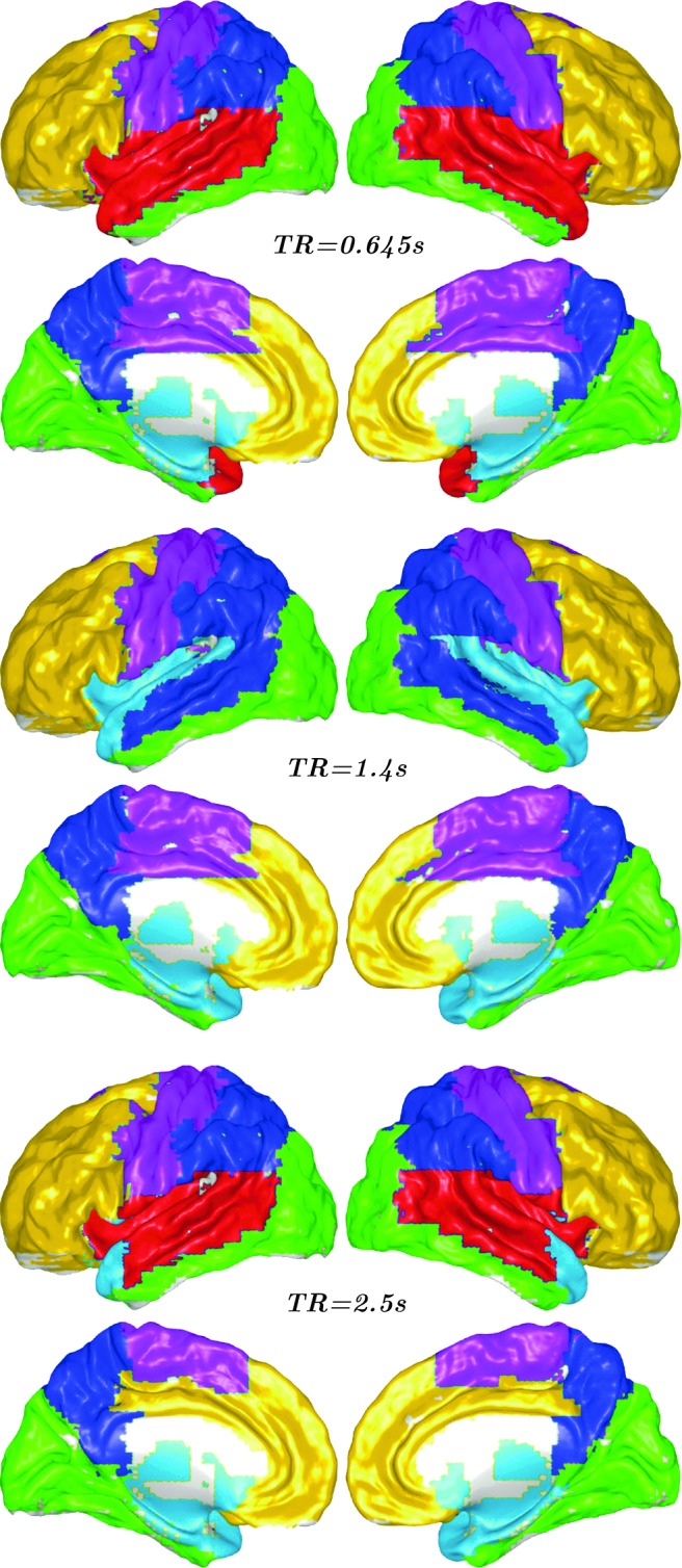
Division in communities of mutually informative regions for different TRs.

At this point, it is interesting to see how the different measures of GC are affected by the size of the dataset. We computed PCGC, CGC, and pairwise GC for three different parcellations of the cortex, in 7, 17, and 90 regions (Fig. 5). When the number of regions is low, there is high correlation of the values of PCGC (n_d=2 was chosen in this case) with both pairwise GC (r=0.90) and CGC (r=0.89). When the regions are increased to 17, the correlation with pairwise CG drops to 0.35 while the one with CGC stays high (0.79). With 90 regions, the correlation with pairwise GC is 0.25, and the one with PCGC is 0.79. Despite the still high correlation, the slope of the fitting line for PCGC versus CGC is lower, confirming that the redundancy has the effect of reducing the detection of Granger-causal influences when a fully conditioned approach is employed (Marinazzo et al., 2010).

FIG. 5.

Top: the values of CGC (red) and pairwise GC (black) are plotted against the values of PCGC for different parcellations of the brain. (A) Yeo 7 template. (B) Yeo 17 template. (C) AAL 90 template. Bottom: connectivity matrices between the 90 regions of the AAL template obtained by CGC (D) and PCGC (E), after family-wise error (FWE) correction, p<0.01.

When we compare the connectivity matrix for CGC and PCGC for the 90 regions, after family-wise error correction for multiple comparisons, we see that the PCGC matrix is more structured, still remaining sparse.

EEG data

Also for EEG data, the curve of the information gain decays rapidly with the number of variables used for conditioning (Fig. 6B). Contrarily to what happens in fMRI data, here the neighboring electrodes are most often chosen as the most informative for each target, though the extension of this neighborhood is different across the scalp (Fig. 6C). Also in this case, the connectivity matrix is sparse (Fig. 6A), and PCGC and CGC values are highly correlated, r=0.88 (Fig. 6B, inset).

FIG. 6.

(A) Connectivity matrix for PCGC, FWE corrected, p<0.01, for the electroencephalogram dataset. (B) Mutual information gain when an additional variable is used for conditioning, averaged for all the targets. Inset: plot of PCGC versus CGC. (C) The relative frequency with which other electrodes were chosen among the first 10 most informative ones for each electrode.

Discussion and Conclusions

This study has proposed a solution to one of the problems inherent to the application of GC to neuroimaging datasets, showing that partial conditioning on a small number of the most informative variables for the driver node leads to results very close to the fully multivariate analysis and even better in case of the small number of samples, especially when the pattern of causalities is sparse. Anatomical studies have shown that the axonal connectivity of the cortex is generally sparse (Hagmann et al., 2008), and FC studies have revealed the highly clustered and redundant structure of the brain as a dynamical system. The approach proposed here is indeed optimized, taking into account these characteristics.

Another challenge for GC application to fMRI data is downsampling and hemodynamic confound. The downsampling is so far an unavoidable flaw in fMRI, and it has been confirmed here that a significant amount of information on the future of each target variable is lost when the TR is long. The hemodynamic response function varies across different brain regions, sessions, and subjects. Here a blind deconvolution method for resting-state fMRI data (Wu et al., 2013) was applied, allowing the detection the EC network at a neural level (Matlab code is available in http://users.ugent.be/∼dmarinaz/code.html).

Modularity is an important organizational principle of complex brain networks (Bullmore and Sporns, 2009). Brain communities are sets of regions that are highly connected among each other while connections between members of different communities are less dense. Investigating modularity hence might be helpful to uncover the functional segregation of neural information (Sporns, 2013). Recently, convergence and divergence modular structures have been documented in human anatomical (Gong et al., 2009; Hagmann et al., 2008) and functional connectomes (He et al., 2009; Meunier et al., 2009). In those studies, modules related to the primary brain functions, such as visual, auditory, sensorimotor, subcortical, and the default-mode systems, were regularly detected. In this study, we also found a modular organization, which mainly involved the visual, auditory, limbic, and subcortical systems, separated the anterior default-mode network. This default-mode subsystem is consistent with our previous findings (Liao et al., 2011), thus providing an evidence for functional anatomic fractionation of the brain's default-mode network (Andrews-Hanna et al., 2010; Andrews-Hanna, 2011). Here we propose a modular structure based on the informational content, providing new insights into the understanding of functional segregation of brain networks at rest.

This study has reported results for 90 ROIs obtained by means of an anatomical template; for finer resolutions, with templates with a higher number of regions, or even at a single-voxel level, further modifications and improvement to this technique could be in order.

When electroencephalographic recordings are concerned, the idea that scalp conductivity could play a prominent role as a common source of information seems confirmed in this case.

This approach is based on the equivalence of linear GC and transfer entropy for gaussianly distributed variables. For resting-state fMRI, which we believe that it will be the main target of this approach, this equivalence can be close to be fulfilled. Anyway, also for another type of non-Gaussian data, this approach remains valid: the loss of accuracy due to the only approximate equivalence is negligible compared to the conceptual and computational improvements that make the application of GC possible also in presence of strong redundancy. Nonetheless, future work will be required to make this approach exact for all kind of data distribution and to use the exact formulation for the calculation of the transfer entropy.

Acknowledgments

This research was supported by the China Scholarship Council (grant number 2011607033 for G.R.W.) and the Natural Science Foundation of China (grant number 81201155 for W.L).

Author Disclosure Statement

No competing financial interests exist.

References

- Andrews-Hanna JR. The brain's default network and its adaptive role in internal mentation. Neuroscientist. 2011;8:251–270. doi: 10.1177/1073858411403316. [DOI] [PMC free article] [PubMed] [Google Scholar]
- Andrews-Hanna JR. Reidler JS. Sepulcre J. Poulin R. Buckner RL. Functional-anatomic fractionation of the brain's default network. Neuron. 2010;65:550–562. doi: 10.1016/j.neuron.2010.02.005. [DOI] [PMC free article] [PubMed] [Google Scholar]
- Barnett L. Barrett AB. Seth AK. Granger causality and transfer entropy are equivalent for Gaussian variables. Phys Rev Lett. 2009;103:238701. doi: 10.1103/PhysRevLett.103.238701. [DOI] [PubMed] [Google Scholar]
- Barrett AB. Barnett L. Seth AK. Multivariate Granger causality and generalized variance. Phys Rev E. 2010;81:041907. doi: 10.1103/PhysRevE.81.041907. [DOI] [PubMed] [Google Scholar]
- Blondel VD. Guillaume JL. Lambiotte R. Lefebvre E. Fast unfolding of communities in large networks. J Stat Mech Theory Exp. 2008;2008:P10008. [Google Scholar]
- Bullmore E. Sporns O. Complex brain networks: graph theoretical analysis of structural and functional systems. Nat Rev Neurosci. 2009;10:186–198. doi: 10.1038/nrn2575. [DOI] [PubMed] [Google Scholar]
- Chen Y. Bressler S. Ding M. Frequency decomposition of conditional Granger causality and application to multivariate neural field potential data. J Neurosci Methods. 2006;150:228. doi: 10.1016/j.jneumeth.2005.06.011. [DOI] [PubMed] [Google Scholar]
- Deshpande G. LaConte S. James GA. Peltier S. Hu X. Multivariate Granger causality analysis of fMRI data. Hum Brain Mapp. 2008;30:1361–1373. doi: 10.1002/hbm.20606. [DOI] [PMC free article] [PubMed] [Google Scholar]
- Faes L. Nollo G. Porta A. Information-based detection of nonlinear Granger causality in multivariate processes via a nonuniform embedding technique. Phys Rev E. 2011;83(5 Pt 1):051112. doi: 10.1103/PhysRevE.83.051112. [DOI] [PubMed] [Google Scholar]
- Friston K. Moran R. Seth AK. Analysing connectivity with Granger causality and dynamic causal modelling. Curr Opin Neurobiol. 2012:00184–00185. doi: 10.1016/j.conb.2012.11.010. [DOI] [PMC free article] [PubMed] [Google Scholar]
- Friston KJ. Functional and effective connectivity: a review. Brain Connect. 2011;1:13–36. doi: 10.1089/brain.2011.0008. [DOI] [PubMed] [Google Scholar]
- Geweke JF. Measures of conditional linear dependence and feedback between time series. J Am Stat Assoc. 1984;79:907–915. [Google Scholar]
- Goebel R. Roebroeck A. Kim DS. Formisano E. Investigating directed cortical interactions in time-resolved fMRI data using vector autoregressive modeling and Granger causality mapping. Magn Reson Imaging. 2003;21:1251–1261. doi: 10.1016/j.mri.2003.08.026. [DOI] [PubMed] [Google Scholar]
- Goldberger AL. Amaral LAN. Glass L. Hausdorff JM. Ivanov PCh. Mark RG. Mietus JE. Moody GB. Peng C-K. Stanley HE. PhysioBank, PhysioToolkit, and PhysioNet: components of a new research resource for complex physiologic signals. Circulation. 2000;101:e215–e220. doi: 10.1161/01.cir.101.23.e215. [DOI] [PubMed] [Google Scholar]
- Gong G. He Y. Concha L. Lebel C. Gross DW. Evans AC. Beaulieu C. Mapping anatomical connectivity patterns of human cerebral cortex using in vivo diffusion tensor imaging tractography. Cerebral Cortex. 2009;19:524–536. doi: 10.1093/cercor/bhn102. [DOI] [PMC free article] [PubMed] [Google Scholar]
- Granger CWJ. Investigating causal relations by econometric models and cross-spectral methods. Econometrica. 1969;37:424–438. [Google Scholar]
- Hagmann P. Cammoun L. Gigandet X. Meuli R. Honey CJ. Wedeen VJ, et al. Mapping the structural core of human cerebral cortex. PLoS Biol. 2008;6:e159. doi: 10.1371/journal.pbio.0060159. [DOI] [PMC free article] [PubMed] [Google Scholar]
- Hartman D. Hlinka J. Palus M. Mantini D. Corbetta M. The role of nonlinearity in computing graph-theoretical properties of resting-state functional magnetic resonance imaging brain networks. Chaos. 2011;21:013119. doi: 10.1063/1.3553181. [DOI] [PMC free article] [PubMed] [Google Scholar]
- He Y. Chen Z. Gong G. Evans A. Neuronal networks in Alzheimer's disease. Neuroscientist. 2009;15:333–350. doi: 10.1177/1073858409334423. [DOI] [PubMed] [Google Scholar]
- Hlavácková-Schindler K. Equivalence of Granger causality and transfer entropy: a generalization. Appl Math Sci. 2011;5:3637–3648. [Google Scholar]
- Hlinka J. Palus M. Vejmelka M. Mantini D. Corbetta M. Functional connectivity in resting-state fMRI: is linear correlation sufficient? NeuroImage. 2011;54:2218–2225. doi: 10.1016/j.neuroimage.2010.08.042. [DOI] [PMC free article] [PubMed] [Google Scholar]
- Kus R. Kaminski M. Blinowska KJ. Determination of EEG activity propagation: pair-wise versus multichannel estimate. IEEE Trans Biomed Eng. 2004;51:1501–1510. doi: 10.1109/TBME.2004.827929. [DOI] [PubMed] [Google Scholar]
- Liao W. Ding J. Marinazzo D. Xu Q. Wang Z. Yuan C. Zhang Z. Lu G. Chen H. Small-world directed networks in the human brain: multivariate Granger causality analysis of resting-state fMRI. NeuroImage. 2011;54:2683–2694. doi: 10.1016/j.neuroimage.2010.11.007. [DOI] [PubMed] [Google Scholar]
- Liao W. Mantini D. Zhang Z. Pan Z. Ding J. Gong Q, et al. Evaluating the effective connectivity of resting state networks using conditional Granger causality. Biol Cybern. 2010;102:57–69. doi: 10.1007/s00422-009-0350-5. [DOI] [PubMed] [Google Scholar]
- Marinazzo D. Liao W. Pellicoro M. Stramaglia S. Grouping time series by pairwise measures of redundancy. Phys Lett A. 2010;374:4040–4044. [Google Scholar]
- Marinazzo D. Pellicoro M. Stramaglia S. Causal information approach to partial conditioning in multivariate data sets. Comput Math Methods Med. 2012;2012:303601. doi: 10.1155/2012/303601. [DOI] [PMC free article] [PubMed] [Google Scholar]
- Meunier D. Achard S. Morcom A. Bullmore E. Age-related changes in modular organization of human brain functional networks. NeuroImage. 2009;44:715–723. doi: 10.1016/j.neuroimage.2008.09.062. [DOI] [PubMed] [Google Scholar]
- Price CJ. Friston KJ. Degeneracy and cognitive anatomy. Trends Cogn Sci. 2002;6:416–421. doi: 10.1016/s1364-6613(02)01976-9. [DOI] [PubMed] [Google Scholar]
- Ritter P. Schirner M. McIntosh AR. Jirsa V. The Virtual Brain Integrates Computational Modelling and Multimodal Neuroimaging. Brain Connect. 2013;3:121–145. doi: 10.1089/brain.2012.0120. [DOI] [PMC free article] [PubMed] [Google Scholar]
- Runge J. Heitzig J. Marwan N. Kurths J. Quantifying causal coupling strength: a lag-specific measure for multivariate time series related to transfer entropy. Phys Rev E. 2012;86:061121. doi: 10.1103/PhysRevE.86.061121. [DOI] [PubMed] [Google Scholar]
- Schalk G. McFarland DJ. Hinterberger T. Birbaumer N. Wolpaw JR. BCI2000: a general-purpose brain-computer interface (BCI) system. IEEE Trans Biomed Eng. 2004;51:1034–43. doi: 10.1109/TBME.2004.827072. [DOI] [PubMed] [Google Scholar]
- Sporns O. Network attributes for segregation and integration in the human brain. Curr Opin Neurobiol. 2013:00189–4. doi: 10.1016/j.conb.2012.11.015. [DOI] [PubMed] [Google Scholar]
- Stefanescu RA. Jirsa VK. A low dimensional description of globally coupled heterogeneous neural networks of excitatory and inhibitory neurons. PLoS Comput Biol. 2008;4:e1000219. doi: 10.1371/journal.pcbi.1000219. [DOI] [PMC free article] [PubMed] [Google Scholar]
- Wu G. Liao W. Stramaglia S. Ding J. Chen H. Marinazzo D. A blind deconvolution approach to recover effective connectivity brain networks from resting state fMRI data. Med Image Anal. 2013;17:365–74. doi: 10.1016/j.media.2013.01.003. [DOI] [PubMed] [Google Scholar]
- Zhou Z. Chen Y. Ding M. Wright P. Lu Z. Liu Y. Analyzing brain networks with PCA and conditional Granger causality. Hum Brain Mapp. 2008;30:2197–2206. doi: 10.1002/hbm.20661. [DOI] [PMC free article] [PubMed] [Google Scholar]