A HIERARCHICAL MAX-STABLE SPATIAL MODEL FOR EXTREME PRECIPITATION

Abstract

Extreme environmental phenomena such as major precipitation events manifestly exhibit spatial dependence. Max-stable processes are a class of asymptotically-justified models that are capable of representing spatial dependence among extreme values. While these models satisfy modeling requirements, they are limited in their utility because their corresponding joint likelihoods are unknown for more than a trivial number of spatial locations, preventing, in particular, Bayesian analyses. In this paper, we propose a new random effects model to account for spatial dependence. We show that our specification of the random effect distribution leads to a max-stable process that has the popular Gaussian extreme value process (GEVP) as a limiting case. The proposed model is used to analyze the yearly maximum precipitation from a regional climate model.

1. Introduction

Spatial statistical techniques are crucial for accurately quantifying the likelihood of extreme events and monitoring changes in their frequency and intensity. Extreme events are by definition rare, therefore estimation of local climate characteristics can be improved by borrowing strength across nearby locations. While methods for univariate extreme data are well-developed, modeling spatially-referenced extreme data is an active area of research. Max-stable processes (de Haan and Ferreira, 2006) are the natural infinite-dimensional generalization of the univariate generalized extreme value (GEV) distribution. Just as the only limiting distribution of the scaled maximum of independent univariate random variables is the GEV, the scaled maximum of independent copies of any stochastic process can only converge to a max-stable process. Max-stable process models for spatial data may be constructed using the spectral representation of de Haan (1984). Max-stable processes built from this representation were first used for spatial analysis by Smith (1990). Since then, a handful of subsequent spatial max-stable process models have been proposed, notably that of Schlather (2002) and Kabluchko et al. (2009), who proposed a more general construction that includes several other known models as special cases. Applications of spatial max-stable processes include Coles (1993), Buishand et al. (2008), and Blanchet and Davison (2011).

Because closed-form expressions for the likelihoods associated with spatial max-stable processes are not available, parameter estimation and inference is problematic. Taking advantage of the availability of bivariate densities, Padoan et al. (2010) suggest maximum pairwise likelihood estimation and asymptotic inference based on a sandwich matrix (composed of expected derivatives of the composite likelihood function) to properly account for using a pairwise likelihood when computing standard errors (Godambe and Heyde, 1987). Recently, Genton et al. (2011) extend this approach using composite likelihood based on trivariate densities. The problem of spatial prediction, conditional on observations, for max-stable random fields (analogous to Kriging for Gaussian processes) has also proven difficult. The recent conditional sampling algorithm of Wang and Stoev (2010a) is capable of producing both predictions and prediction standard errors for most spatial max-stable models of practical interest, subject to discretization errors that can be made arbitrarily small.

Bayesian estimation and inference for max-stable process models for spatial data on a continuous domain has been elusive. Implementing these models in a fully-Bayesian framework has several advantages, including incorporation of prior information and natural uncertainty assessment for model parameters and predictions. Approximate Bayesian methods based on asymptotic properties of the pairwise likelihood function are possible. Ribatet et al. (2012) use an estimated sandwich matrix to adjust the Metropolis ratio within an MCMC sampler, while Shaby (2012) rotates and scales the MCMC sample post-hoc and Smith and Stephenson (2009) use pairwise likelihoods without adjustment. Bayesian models that are not based on max stable processes have been used for analysis of extreme values with spatial structure. Cooley et al. (2007) uses a hierarchical model with a conditionally-independent generalized Pareto likelihood, incorporating all spatial dependence through Gaussian process priors on the generalized Pareto likelihood parameters. Spatial dependence has also been achieved through Bayesian Gaussian copula models (Sang and Gelfand, 2010) and through a more flexible copula based on a Dirichlet process construction (Fuentes et al., 2012).

We develop a new hierarchical Bayesian model for analyzing max-stable processes. The responses are modeled as independent univariate GEV conditioned on spatial random effects with positive stable random effect distribution. Positive stable random effects have been used to model multivariate extremes with finite dimensions (Fougerès et al., 2009; Stephenson, 2009). We extend this approach to accommodate data on a continuous spatial domain. We show that the resulting model is max-stable marginally over the random effects, and that a limiting case of this construction provides a finite-dimensional approximation to the well-known Gaussian extreme value process (GEVP) of Smith (1990), often referred to as the “Smith process”. Lower-dimensional representations have previously been proposed for high-dimensional extremes in various settings (Pickands, 1981; Deheuvels, 1983; Schlather and Tawn, 2002; Ehlert and Schlather, 2008; Wang and Stoev, 2010a,b; Oesting et al., 2011; Engelke et al., 2011). Our construction permits analysis of the joint distribution of all observations, and thus can produce straight-forward predictions at unobserved locations. Because we use a hierarchical model to represent the spatial max-stable process, a Bayesian implementation is a natural choice. This allows us to model underlying marginal structures as flexibly as we like, in addition to automatic pooling of information and uncertainty propagation. Also, the proposed framework permits representing the the spatial process using a lower-dimensional representation, which leads to efficient computing for large spatial data sets.

The remainder of the paper proceeds as follows. Section 2 describes the model, which is compared to the GEVP in Section 3. The method is evaluated using a simulation study in Section 4. In Section 5, we use the proposed method to analyze yearly maximum precipitation using regional climate model output from the North American Regional Climate Change Assessment Program (NARCCAP) in the eastern US. Section 6 concludes.

2. The hierarchical max-stable process model

2.1. Spatial random effects model

Let Y (s) be the extreme value at location s, defined over the region $\mathbf{s}\in \mathcal{D}\subset {\mathcal{R}}^2$. Here we describe a max-stable model for Y (s) assuming that it is a block-maximum, that is, the maximum of many observations taken at location s, such as the yearly maximum of daily precipitation levels. However, we note that max-stable models are increasingly being used to model extreme individual observations using a points above threshold approach (Huser and Davison, 2012), and the residual max-stable process model described here may be applicable to this type of analysis as well. We describe a model for a single realization of the process, and extend to multiple independent realizations in Section 2.3.

Assuming the process is max-stable, then the marginal distribution of Y (s) is GEV[μ(s), σ(s), ξ(s)], where μ(s) is the location, σ(s) > 0 is the scale, and ξ(s) is the shape (GEV distribution is described in Appendix A.1). Equivalently (Resnick, 1987), we may express $Y\left(\mathbf{s}\right)=\mu \left(\mathbf{s}\right)+\frac{\sigma \left(\mathbf{s}\right)}{\xi \left(\mathbf{s}\right)}\left[X{\left(\mathbf{s}\right)}^{\xi \left(\mathbf{s}\right)}-1\right]$, where X(s) is the residual max-stable process with unit Fréchet margins, i.e., X(s) ~ GEV(1,1,1). To allow for both non-spatial and spatial residual variability, we model X(s) as the product X(s) = U(s)θ(s). Borrowing a term from geostatistics, we refer to U(s) as the nugget effect since it accounts for non-spatial variation due to measurement error or other small-scale features. The nugget is modeled as $U\left(\mathbf{s}\right)\stackrel{iid}{\sim }\mathrm{GEV}(1,\alpha ,\alpha )$, where, as described in detail below, the parameter α ∈ (0, 1) controls the relative contribution the nugget effect.

Residual spatial dependence is captured by θ(s). We express the spatial process as a function of a linear combination of L kernel basis functions w_l(s) ≥ 0, scaled so that ${\sum }_{l=1}^L{w}_l\left(\mathbf{s}\right)=1$ for all s. The spatial process is $\theta \left(\mathbf{s}\right)={\left[{\sum }_{l=1}^L{A}_l{w}_l{\left(\mathbf{s}\right)}^{1∕\alpha }\right]}^{\alpha }$, where A_l are the basis function coefficients. To ensure max-stability and Fréchet marginal distributions, the random effects A_l follow the positive stable distribution with density p(A|α) which has Laplace transformation ${\int }_0^{\infty }\text{exp}(-At)p(A\mid \alpha )dA=\text{exp}(-t^{\alpha })$. We denote this as A_l ~ PS(α). Although p(A|α) has no closed form, it possesses the essential feature that if $A_1,\dots ,A_T\stackrel{iid}{\sim }\mathrm{PS}\left(\alpha \right)$, then (A₁ + ... + A_T)/T^1/α ~ PS(α). Appendix A.2 verifies that this model for X(s) is max-stable with unit Fréchet marginal distributions.

Marginalizing over the nugget terms U(s) gives the hierarchical model

$$\begin{array}{cc}\hfill Y\left({\mathbf{s}}_i\right)\mid A_1,\dots ,A_L& \stackrel{indep}{\sim }\mathrm{GEV}[{\mu }^{\ast }\left({\mathbf{s}}_i\right),{\sigma }^{\ast }\left({\mathbf{s}}_i\right),{\xi }^{\ast }\left({\mathbf{s}}_i\right)]\hfill \\ \hfill A_l& \stackrel{iid}{\sim }\mathrm{PS}\left(\alpha \right)\hfill \end{array}$$ (2.1)

where ${\mu }^{\ast }\left(\mathbf{s}\right)=\mu \left(\mathbf{s}\right)+\frac{\sigma \left(\mathbf{s}\right)}{\xi \left(\mathbf{s}\right)}\left[\theta {\left(\mathbf{s}\right)}^{\xi \left(\mathbf{s}\right)}-1\right]$, σ*(s) = ασ(s)θ(s)^ξ(s), and ξ*(s) = αξ(s). The responses are conditionally independent given the random effects A. The effect of conditioning on A = (A₁, ..., A_L)^T, and thus the spatial process θ, is to move spatial dependence from the residuals to a random effect in the GEV parameters. Marginalizing over the random effects induces spatial dependence. The joint distribution function of the residual process X at n locations s₁, ..., s_n is

$$\mathrm{P}(X\left({\mathbf{s}}_i\right)<c_i,i=1,\dots ,n)=\text{exp}\left\{-\sum _{l=1}^L{\left[\sum _{i=1}^n{\left(\frac{w_l\left({\mathbf{s}}_i\right)}{c_i}\right)}^{1∕\alpha }\right]}^{\alpha }\right\}.$$ (2.2)

Therefore, although this is a process model defined on a continuous spatial domain, the finite-dimensional distributions are multivariate GEV (MGEV) with asymmetric logistic dependence function (Tawn, 1990).

Spatial dependence is often summarized by the extremal coefficient (Smith, 1990). The pairwise extremal coefficient ϑ(s_i, s_j) ∈ [1, 2] is defined by the relationship

$$P(X\left({\mathbf{s}}_i\right)<c,X\left({\mathbf{s}}_j\right)<c)=P{(X\left({\mathbf{s}}_i\right)<c)}^{\vartheta ({\mathbf{s}}_i,{\mathbf{s}}_j)}.$$ (2.3)

If X(s_i) and X(s_j) are independent, then ϑ(s_i, s_j) = 2; in contrast, if X(s_i) and X(s_j) are completely dependent, then ϑ(s_i, s_j) = 1. The extremal coefficient introduced by (2.1) is

$$\vartheta ({\mathbf{s}}_i,{\mathbf{s}}_j)=\sum _{l=1}^L{\left(w_l{\left({\mathbf{s}}_i\right)}^{1∕\alpha }+w_l{\left({\mathbf{s}}_j\right)}^{1∕\alpha }\right)}^{\alpha }.$$ (2.4)

Therefore, the extremal coefficient is the sum (over the L kernels) of the L^1/α norms of the vectors [w_l(s_i), w_l(s_j)].

To see how α controls the nugget effect, consider two observations at the same location, s_i = s_j. The two observations share the same kernels, w_l(s_i) = w_l(s_j) and thus θ(s_i) = θ(s_j), but have different nugget terms U(s_i) ≠ U(s_j). In this case, the extremal coefficient is 2^α. If α = 1, then the nugget dominates and ϑ(s_i, s_j) = 2 for all pairs of locations, regardless of their spatial locations (since ${\sum }_{l=1}^L{w}_l\left(\mathbf{s}\right)=1$ for all s). If α = 0, then ϑ(s_i, s_j) = 1 when s_i = s_j, and there is no nugget effect. The characteristics of the model are shown graphically in Figure 1. In these random draws from the model, we see the process is very smooth for α = 0.1 and has little discernable spatial pattern with α = 0.9.

Fig 1.

Random draws on a 50 × 50 grid from the random effect model for various α. Each sample has a knot at each data point, GEV parameters μ(s) = log[σ(s)] = 0 and ξ(s) = –0.1, and bandwidth τ = 2.

The parameter α clearly plays an important role in this model. It determines the magnitude of the nugget effect, the form of spatial dependence function in (2.4), and the shape and scale of the conditional distributions in (2.1). To illustrate the links between the contribution of α to these aspects of the model, we consider the extreme cases with α = 0 and α = 1. With α = 1, p(A|α) concentrates its mass on A = 1, and thus $\theta \left(\mathbf{s}\right)={\sum }_{l=1}^L{w}_l\left(\mathbf{s}\right)=1$. In this case, the conditional and marginal GEV parameters are the same, e.g., μ*(s) = μ(s), there is no residual dependence with θ(s_i, s_j) = 2, and thus $Y\left(\mathbf{s}\right)\stackrel{indep}{\sim }\mathrm{GEV}[\mu \left(\mathbf{s}\right),\sigma \left(\mathbf{s}\right),\xi \left(\mathbf{s}\right)]$. On the other hand, if α ≈ 0 then the conditional scale σ*(s) ≈ 0 and Y(s) ≈ μ*(s), a continuous spatial process with strong small-scale spatial dependence θ(s, s) ≈ 1.

Spatial prediction (analogous to Kriging) at a new location s* is straight-forward under this hierarchical model. Predictions are made by simply computing $\theta \left({\mathbf{s}}^{\ast }\right)={\left[{\sum }_{l=1}^L{A}_l{w}_l{\left({\mathbf{s}}^{\ast }\right)}^{1∕\alpha }\right]}^{\alpha }$, and then sampling Y(s*) from the independent GEV in (2.1). Repeating this at every MCMC iteration gives samples from the posterior predictive distribution of Y(s*).

2.2. Kernel and knot selection

Although other kernels are possible, we use a scaled version of the Gaussian kernel

$$K(\mathbf{s}\mid {\mathbf{v}}_l,\tau )=\frac{1}{2\pi {\tau }^2}\text{exp}\left[-\frac{1}{2{\tau }^2}{(\mathbf{s}-{\mathbf{v}}_l)}^T(\mathbf{s}-{\mathbf{v}}_l)\right],$$ (2.5)

where ${\mathbf{v}}_1,\dots ,{\mathbf{v}}_L\in {\mathcal{R}}^2$ are spatial knots and τ > 0 is the kernel bandwidth. To ensure that the kernels sum to one at each location, the kernels are scaled as

$$w_l\left(\mathbf{s}\right)=\frac{K(\mathbf{s}\mid {\mathbf{v}}_l,\tau )}{\sum _{j=1}^{L}K(\mathbf{s}\mid {\mathbf{v}}_j,\tau )}.$$ (2.6)

The knots are taken as a fixed and regularly-spaced grid of points covering the spatial domain. Section 3 shows that this choice of kernel function and knot distribution gives the GEVP as a limiting case. Even with a regular grid of knots, the extremal coefficient is non-stationary, i.e., ϑ(s_i, s_j) is not simply a function of ∥s_i – s_j∥. For example, w(s_i) may not equal w(s_j) if s_i is close to a knot and s_j is not. This discretization artifact dissipates for large L.

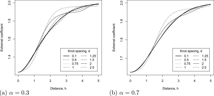
While the extremal coefficient does not fully characterize spatial dependence, it is useful for guiding knot selection. Knot selection poses a trade-off between computational burden with too many knots and poor fit with too few knots. Consider the case of a Gaussian kernel with bandwidth τ = 1 and knots on a large rectangular grid with grid spacing d. Figure 2 plots the extremal coefficient for points (0, 0) and (0, h) as a function of separation distance h. The extremal coefficient has nearly an identical shape for all d less than or equal to τ. For d = 1.25τ, the extremal coefficient differs slightly from the fine grids, and for d > 1.25τ the extremal coefficient deviates considerably from the fine grids, especially for small α. These results will scale for other τ, therefore a rule of thumb is to select the knots so that the grid spacing is approximately equal to the kernel bandwidth. Knot selection is discussed further in Section 4.

Fig 2.

Extremal coefficient ϑ(s₁, s₂), where s₁ = (0, 0), s₂ = (0, h), the kernel bandwidth is τ = 1, and the knots form a rectangular grid with grid spacing d.

2.3. Adaption for the NARCCAP data

In Section 5 we analyze climate model output for T > 1 years, which requires additional notation. Denote Y_t(s) as the response for year t and site s. Assuming the years are independent and identically distributed (over years, not space), gives

$$\begin{array}{cc}\hfill Y_t\left({\mathbf{s}}_i\right)\mid A_{1t},\dots ,A_{Lt}& \stackrel{indep}{\sim }\mathrm{GEV}[{\mu }_t^{\ast }\left({\mathbf{s}}_i\right),{\sigma }_t^{\ast }\left({\mathbf{s}}_i\right),{\xi }^{\ast }\left({\mathbf{s}}_i\right)]\hfill \\ \hfill A_{lt}& \stackrel{iid}{\sim }\mathrm{PS}\left(\alpha \right)\hfill \end{array}$$ (2.7)

where ${\theta }_t\left(\mathbf{s}\right)={\left[{\sum }_{l=1}^L{A}_{lt}{w}_l{\left(\mathbf{s}\right)}^{1∕\alpha }\right]}^{\alpha }$ is the spatial random effect for year t, ${\mu }_t^{\ast }\left(\mathbf{s}\right)=\mu \left(\mathbf{s}\right)+\frac{\sigma \left(\mathbf{s}\right)}{\xi \left(\mathbf{s}\right)}\left({\theta }_t{\left(\mathbf{s}\right)}^{\xi \left(\mathbf{s}\right)}-1\right)$, ${\sigma }_t^{\ast }\left(\mathbf{s}\right)=\alpha \sigma \left(\mathbf{s}\right){\theta }_t{\left(\mathbf{s}\right)}^{\xi \left(\mathbf{s}\right)}$, and ξ*(s) = αξ(s). Note that while the GEV parameters conditioned on θ_t(s) in (2.7) vary by year, marginally, Y_t(s) ~ GEV[μ(s), σ(s), ξ(s)] for all t.

Gaussian process priors are used for the GEV parameters μ(s), γ(s) = log[σ(s)], and ξ(s). The Gaussian process μ has mean x(s)^Tβ_μ, where x(s) includes the spatial covariates such as elevation. The spatial covariance of μ is Matérn (Banerjee et al., 2004; Cressie, 1993; Gelfand et al., 2010) with variance ${\delta }_{\mu }^2>0$, range ρ_μ > 0, and smoothness ν_μ > 0. The other GEV parameters γ(s) and ξ(s) are modeled similarly. In some applications, it may also be desirable to allow for the GEV parameters to evolve over time, perhaps following a separate linear time trend at each location, which would be a straight-forward modification of this model. The MCMC algorithm used to sample from this model is described in Appendix A.3.

3. Connection with the Gaussian extreme value process

The GEVP of Smith (1990) is a well-known spatial max-stable process. In this section, we show that the proposed positive stable random effects model in Section 2 contains this model as a limiting case. The GEVP construction for the residual process is

$$X\left(\mathbf{s}\right)=\text{max}\{h_{1}K(\mathbf{s}\mid {\mathbf{u}}_1,\Sigma ),h_{2}K(\mathbf{s}\mid {\mathbf{u}}_2,\Sigma ),\dots \},$$ (3.1)

where {(h₁, u₁), (h₂, u₂), ...} follows a Poisson process with intensity λ(h, u) = h^–2I(h > 0), and K is a kernel function standardized so that ∫ K(s|u, τ)du = 1 for all s. The construction (3.1) is a special case of the de Haan (de Haan, 1984) spectral representation. A useful analogy is to think of X(s) as the maximum rainfall at site s, generated as the maximum over a countably-infinite number of storms. The k^th storm has center ${\mathbf{u}}_k\in {\mathcal{R}}^2$, intensity h_k > 0, and spatial range given by K(s|u_k, τ).

Under this model, the joint distribution at locations s₁, ..., s_n is

$$\mathrm{P}[X\left({\mathbf{s}}_1\right)<c_1,\dots ,X\left({\mathbf{s}}_n\right)<c_n]=\text{exp}\left[-\int \underset{i}{\text{max}}\left\{\frac{K({\mathbf{s}}_i\mid \mathbf{u},\Sigma )}{c_i}\right\}d\mathbf{u}\right].$$ (3.2)

The GEVP has extremal coefficient

$$\vartheta ({\mathbf{s}}_i,{\mathbf{s}}_j)=\int \text{max}\{K({\mathbf{s}}_i\mid \mathbf{u},\Sigma ),K({\mathbf{s}}_j\mid \mathbf{u},\Sigma )\}d\mathbf{u},$$ (3.3)

which simplifies to $\vartheta ({\mathbf{s}}_i,{\mathbf{s}}_j)=2\Phi \left(\frac{\Vert {\mathbf{s}}_i-{\mathbf{s}}_j\Vert }{2\tau }\right)$ for the Gaussian kernel (2.5). This does not include a nugget effect, since ϑ(s_i, s_j) = 1 if ∥s_i – s_j∥ = 0.

The connection to the model in Section 2 is made by restricting the storm locations to the set of L knot locations {v₁, ..., v_L} and rescaling the kernels to sum to one as in (2.6), giving

$$X\left(\mathbf{s}\right)=\text{max}\{h_1{w}_1\left(\mathbf{s}\right),\dots ,h_L{w}_L\left(\mathbf{s}\right)\}.$$ (3.4)

This amounts to truncating the de Haan spectral representation. If h_l~ GEV(1,1,1), then X(s) is max-stable with joint distribution

$$\mathrm{P}[X\left({\mathbf{s}}_1\right)<c_1,\dots ,X\left({\mathbf{s}}_n\right)<c_n]=\text{exp}\left[-\sum _{l=1}^L\underset{i}{\text{max}}\left\{\frac{w_l\left({\mathbf{s}}_i\right)}{c_i}\right\}\right],$$ (3.5)

which implies that the marginal distributions are unit Fréchet. For equally-spaced knots, this distribution converges weakly to the full GEVP distribution function (3.2) as L increases. We note that this finite approximation could be applied to other max-stable models such as those in Schlather (2002) and Kabluchko et al. (2009) by allowing the functions K to be suitably scaled Gaussian processes, unlike the current approach where K is a kernel function.

Using the model described by (3.5) directly is problematic because it may not yield a proper likelihood. The process (3.4) at n locations X(s₁), ..., X(s_n)} is completely determined by the intensities {h₁, ..., h_L. Therefore, the likelihood for {X(s₁), ..., X(s_n)} requires a map from {X(s₁), ..., X(s_n)} to {h₁, ..., h_L}. This map may not exist, for example if L < n, and generally does not have a closed form. This is common in dimension reduction methods for Gaussian process models (for example, Higdon et al. (1999), Banerjee et al. (2008), and Cressie and Johannesson (2008)).

As with the Gaussian process dimension reduction methods, the model in Section 2 includes both a spatial process (θ) and a non-spatial nugget term (U). Comparing (2.2) and (3.5), we see a result of the nugget effect is that the L^∞ norm (the maximum) in (3.5) is replaced with the L^1/α norm, and that (2.2) converges weakly to (3.5) as α goes to zero. Including a nugget aids in computation as the likelihood becomes a simple product of univariate GEV densities. Including a nugget term also has advantages beyond computation. The GEVP has been criticized as unrealistically smooth (Blanchet and Davison, 2011), and so a nugget may improve fit. Analogously, in the geostatistical literature for Gaussian data a nugget is not required, but is used routinely to account for small-scale phenomena that cannot be captured with a smooth spatial process (Cressie, 1993; Banerjee et al., 2004; Gelfand et al., 2010).

4. Simulation study

In this section, we conduct a simulation study to verify that the MCMC algorithm produces reliable results, to investigate sensitivity to knot selection, and to determine which parameters are the most difficult to estimate. Data and knots are placed on m × m regular grids covering [l, u] × [l, u], denoted $\mathcal{S}(m,l,u)$. For each simulation design, we generate data from the model described in Section 2.3 at the n = 49 locations $\mathcal{S}(7,0,6)$ and T = 10 independent years. The GEV location parameter varies by site following Gaussian process with mean zero, variance one, and exponential spatial correlation exp(–∥s_i – s_j∥/2). Unlike the analysis of the NARCCAP data in Section 5, the GEV scale and shape parameters are assumed to be the same for all sites and fixed at σ(s) = 1 and ξ(s) = 0.2. We fix these parameters in the simulation study for computational purposes, and because these spatially-varying parameters will likely be hard to estimate for these moderately-sized simulated datasets. The simulations vary by the nugget effect (α), the kernel bandwidth (τ), and the number of knots used to generate the data (L₀). The simulation designs are numbered

1. L₀ = 49 knots at $\mathcal{S}(7,0,6)$, α = 0.3, τ = 3

2. L₀ = 49 knots at $\mathcal{S}(7,0,6)$, α = 0.7, τ = 3

3. L₀ = 25 knots at $\mathcal{S}(5,0,6)$, α = 0.3, τ = 3

4. L₀ = 25 knots at $\mathcal{S}(5,0,6)$, α = 0.7, τ = 3

5. L₀ = 10, 000 knots at $\mathcal{S}(100,-1,7)$, α = 0.4, τ = 1

For the first four designs, the number of knots used to generate the data is small enough to permit fitting the model with the correct number of knots. We use these examples to explore sensitivity to knot selection. The final design with L₀ = 10, 000 knots represents the limiting case with more knots than can be fit computationally. Here we fit several course grids of knots and compare performance as the number of knots increases to provide recommendations on the number of knots needed to provide a good approximation to the limiting process.

M = 50 datasets are generated for each simulation design. For each simulated data set, we fit the model with varying number of knots. For the first four designs we compare L = 25 knots at $\mathcal{S}(5,0,6)$ and L = 49 knots at $\mathcal{S}(7,0,6)$ to compare fits with the true knots and either too few (L = 25 for designs 1 and 2) or too many (L = 49 for designs 3 and 4) knots. For the final design we compare fits with 8 knot grids: L = 25 knots at $\mathcal{S}(5,-1,7)$, ..., L = 144 knots at $\mathcal{S}(12,-1,7)$. The spatial covariance parameters for the GEV location have priors ${\delta }_{\mu }^2\sim \text{InvGamma}(0.1,0.1)$ and range ρ_μ ~ InvGamma(0.1,0.1); for this relatively small spatial domain we fix the smoothness parameter ν_μ = 0.5, giving an exponential covariance. The design matrix X includes only the intercept with β_μ ~ N(0, 100²). The GEV log scale and shape are constant across space and have N(0, 1) and N(0, 0.25²) priors, respectively. The residual dependence parameters have priors τ ~ InvGamma(0.1,0.1) and α ~ Unif(0,1).

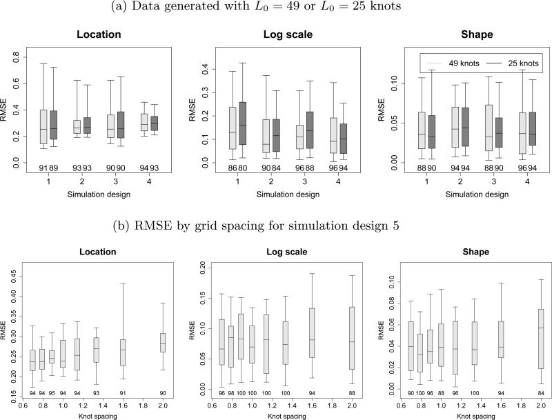
The results are presented in Figure 3. For each dataset, we compute the posterior mean of the GEV parameters at each location, and the mean squared error (MSE) of the posterior means (averaged over the n sites for the spatially-varying GEV location). Figure 3 plots the M = 50 root MSEs and coverage probabilities (averaged over sites for the GEV location).

Fig 3.

Boxplots of root mean squared error (RMSE) for the GEV parameters in the simulation study. The horizontal lines in the boxplots are the 0.05, 0.25, 0.50, 0.75, and 0.95 quantiles of RMSE. Coverage percentages of posterior 95% intervals are given below the boxplots.

For the data generated with L₀ = 25 or L₀ = 49 knots in Figure 3a, the coverage probabilities are generally near the nominal level. With L = 49 knots, the coverage probabilities range from 0.90 to 0.94 for the GEV location. For the first two designs, the model with L = 25 knots has fewer knots than were used to generate the data. This does not have a substantial impact on the estimation of the GEV location. However, using too few knots leads to increased RMSE and under-coverage for the GEV log scale, especially for design 1 with strong spatial dependence. For simulation designs 3 and 4, the model with L = 49 knots has nearly twice as many knots than were used to generate the data. In these cases, the L = 49 model performs nearly as well as the correct L = 25 model. For these simulation settings, we conclude that using too few knots can lead to poor results, especially for the scale parameter, but that including too many knots does not degrade performance.

For the data generated with L₀ = 10, 000 knots in Figure 3b, we use knots grids with L = 25, 36, ..., 144 points. For comparison with the kernel bandwidth, rather than plotting the results by L, we plot results by the spacing between adjacent knots in same column or row, which ranges from 0.70 for L = 144 to 2.00 for L = 25. The coverage probabilities are near or above the nominal level for all grid spacings at or below the bandwidth, τ = 1.0, and the RMSE appears to be fairly constant for all grid spacings at least as small as the bandwidth. Therefore, this appears to be a reasonable rule of thumb for selecting the number of knots.

We also computed RMSE for the spatial dependence parameters α and τ (not shown in Figure 3) for this final case. For α, the average (over data sets) RMSE was 0.049 (coverage percentage 96%), 0.060 (88%), and 0.101 (40%) for grid spacings 0.7, 1.0 and 2.0, respectively. For τ, the average RMSE was 0.102 (88%), 0.107 (90%), and 0.233 (38%) for grid spacings 0.7, 1.0 and 2.0, respectively. As with the GEV parameters, the approximation with the grid spacing at least as small as the bandwidth appears to provide reasonable estimation of the spatial dependence parameters. When too few knots are used, the bandwidth is often over-estimated to compensate for the lack of knots, and thus RMSE is high and coverage is far below the nominal level.

5. Analysis of regional climate model output

To illustrate the proposed method, we analyze climate model output provided by the North American Regional Climate Change Assessment Program (NARCCAP). Our objective is to study changes in extreme precipitation under various climate scenarios in different spatial regions while accounting for residual spatial dependence remaining after allowing for spatially-varying GEV parameters. The data are downloaded from the website http://www.narccap.ucar.edu/index.html. We analyze output from two timeslice experiments. Both runs use the Geophysical Fluid Dynamics Laboratory's AM2.1 climate model with 50km resolution. The model is run separately under historical (1969–2000) and future conditions (2039–2070). Observational data is used for the sea-surface temperature and ice boundary conditions in the historical run. The boundary conditions for the future run are perturbations of the historical boundary conditions. The amount of perturbation is based on a lower resolution climate model. The perturbations assume the A2 emissions scenario (Nakicenovic et al., 2000) which increases CO₂ concentration levels from the current values of about 380 ppm to about 870 ppm by the end of the 21st century.

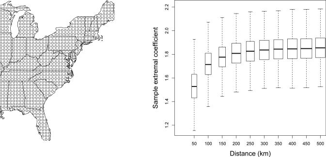
We analyze data for n = 697 grid cells in eastern US shown in Figure 4. For grid cell i with location s_i and year t, we take the annual maximum of the daily precipitation totals as the response, Y_t(s_i). NARCCAP provides eight 3-hour precipitation rates each day, and we compute the daily total by summing these eight values and multiplying by three. To explore the form of residual spatial dependence, we use the madogram (Cooley et al., 2006) function in the SpatialExtremes package in R (www.r-project.org). The madogram converts the observations at each site to have unit Fréchet margins using a rank transformation, and then estimates the pairwise extremal coefficients. Figure 4 plots the estimated extremal coefficients against ∥s_i – s_j∥. This plot clearly shows residual spatial dependence.

Fig 4.

Grid cell centers for the NARCCAP output (left) and madogram extremal coefficient estimate (box width is proportional to the number of observations) for the historical run.

The data from the two runs are analyzed separately using the model described in Section 2. We assume that the process is stationary in time during each period, i.e., the GEV marginal density at each location is constant over time in each simulation period. We use n = L terms with knots at the data points s₁, ..., s_n. The residual dependence parameters have priors τ ~ InvGamma(0.1,0.1) and α ~ Unif(0,1). For both scenarios, all three GEV parameters vary spatially following Gaussian process priors. The covariates for the mean of the GEV parameters, x(s), include the intercept, grid cell latitude, longitude, elevation, and log elevation. The elements of β_μ have independent N(0, 100²) priors. The spatial covariance parameters have priors ${\delta }_j^2\sim \text{InvGamma}(0.1,0.1)$, range ρ_j ~ InvGamma(0.1,0.1), and smoothness ν_j ~ InvGamma(0.1,0.1) for j ∈ {μ, γ, ξ}.

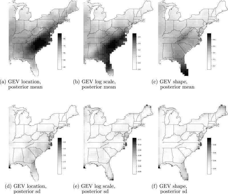
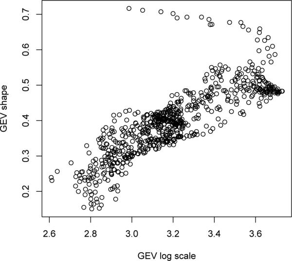
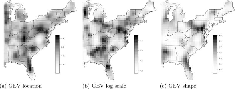
Figure 5 shows the estimated GEV parameters for the historical simulation. The estimated location and log scale parameters are highest in the southeast. The posterior mean of the GEV shape is generally positive, indicating a right-skewed distribution with no upper bound. The estimated shape is the largest in Florida. Comparing the posterior means and standard deviations, there is evidence that all three GEV parameters vary spatially. Figure 6 shows that there is strong positive dependence between the shape and scale as one might expect since for shape in (0,0.5) both the mean and variance of GEV includes the ratio of the scale and shape. For locations with large shapes, there is a negative dependence with the log scale.

Fig 5.

Posterior mean and standard deviation of the GEV location, log scale, and shape parameters for the historical simulation. All units are mm/h.

Fig 6.

Plot of the posterior mean GEV scale versus posterior mean GEV shape at each site.

To formally assess the need for spatially-varying GEV parameters, we also refit the model for the historical simulation using the Bayesian variable selection prior of Reich et al. (2010) to test whether the variance ${\delta }_j^2$ equals small constant ${\Delta }_j^2={0.01}^2$. The test is carried out using the mixture prior ${\delta }_j=g_j{\delta }_j^{\ast }+(1-g_j){\Delta }_0$, where g_j ~ Bernoulli(0.5) and ${\delta }_j^{\ast 2}\sim \text{InvGamma}(0.1,0.1)$. The intuition behind this prior is that if g_j = 1, then ${\delta }_j^2\sim \text{InvGamma}(0.1,0.1)$ and the GEV parameter varies spatially; in contrast, if g₀ = 0, then ${\delta }_j^2={\Delta }_j^2$, and spatial variation after accounting for spatial covariates x is negligible. Therefore, the posterior mean of g_j can be interpreted as the posterior probability that the j^th GEV parameter varies spatially, which can be used to approximate the Bayes factor comparing these model. In the separate mixture prior fit, the posterior probability that the GEV parameters vary spatially was at least 0.99 for all three parameters.

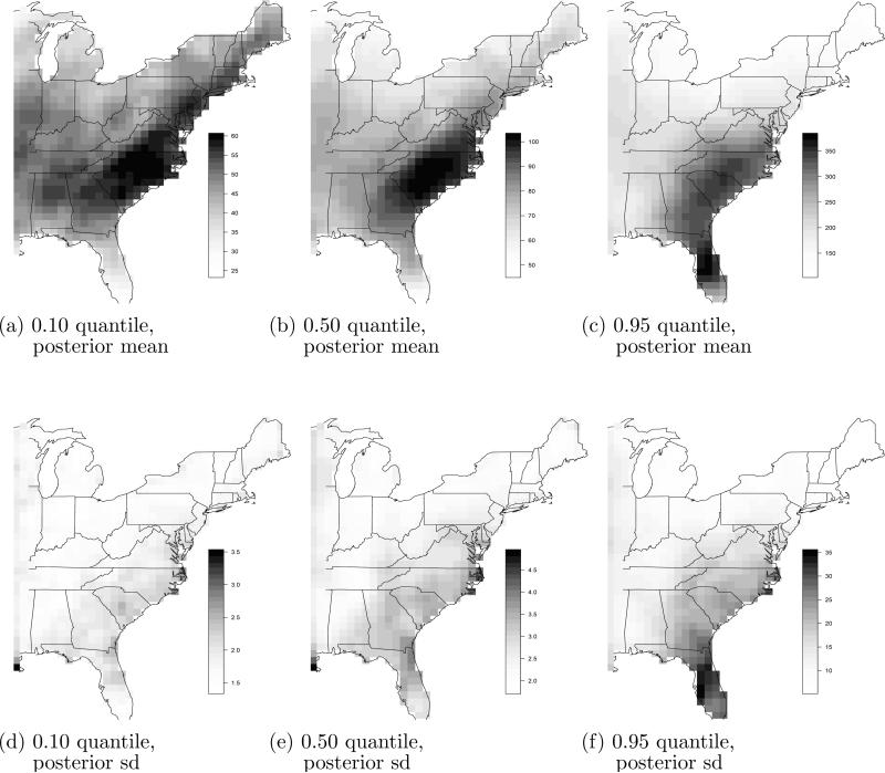
We also aim to quantify changes in extreme quantiles. The q^th quantile at location s is μ(s) + σ(s) [1 – log(1/q)^–ξ(s)]/ξ(s), which is also called the 1/(1 – q) year return level. Figure 7 plots the posterior of various pointwise quantile levels. The large location and scale parameters lead to large medians in the southeast, while the 0.95 quantile is the largest in Florida due to the large shape parameter.

Fig 7.

Posterior mean and standard deviation of the 0.10, 0.50, and 0.95 quantiles for the historical simulation. All units are mm/h

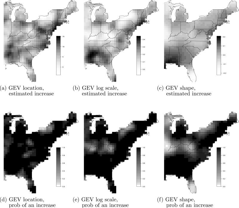
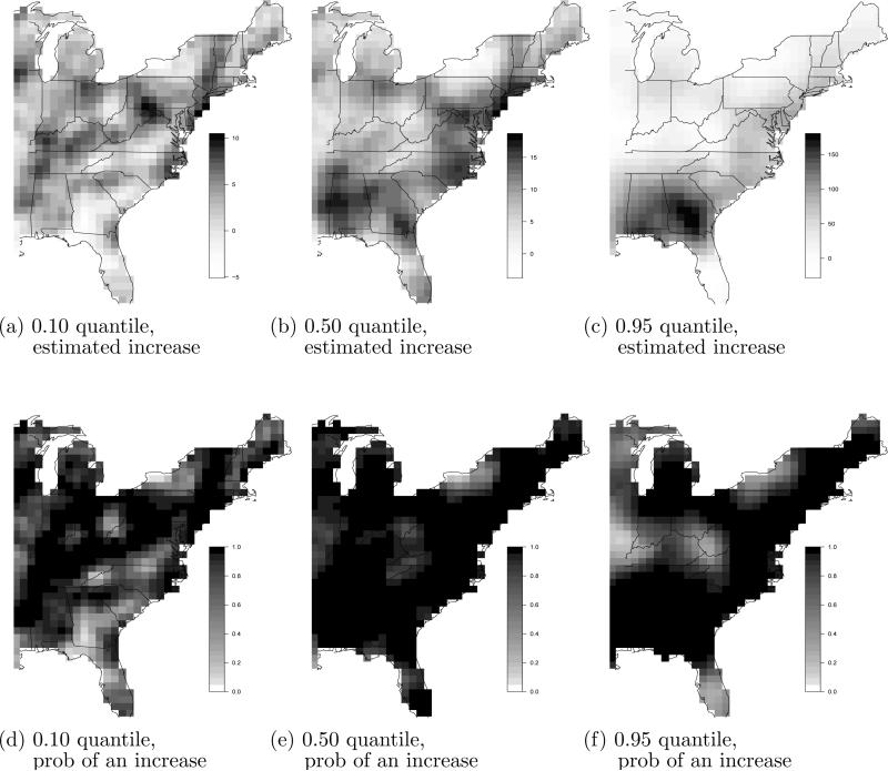
The difference between the historical and future scenarios is summarized in Figures 8 and 9. The estimated GEV location and log scale parameters are larger for the future scenario for the majority of the spatial domain. The increase is the largest in Alabama, Georgia, and New England. The shape parameter also shows an increase in Alabama, but statistically significant decrease in Florida. Figure 9c shows that these changes in GEV parameters lead to an increase in the 0.95 quantile for most of the spatial domain. With the exception of the midwest and southern Florida, the posterior probability of an increase in the 0.95 quantile is near one (Figure 9d), indicating that extremes have a different spatial pattern in the future scenario.

Fig 8.

Posterior mean change from historical to future time simulation and the posterior probability that this change is positive for the GEV location, log scale, and shape parameters. All units are mm/h.

Fig 9.

Posterior mean change from historical to future time simulations and the posterior probability that this change is positive for the 0.10, 0.50, and 0.95 quantiles. All units are mm/h.

Parameter estimates provide evidence of residual dependence: the posterior mean (standard deviation) of α is 0.483 (0.008) and the posterior mean of the spatial range τ is 41.6 (0.4) kilometers. To illustrate the effects of failing to account for residual spatial dependence, we compare these results with the model that ignores spatial dependence in the residuals, i.e., sets α = 1. One effect of accounting for residual dependence is an increase in posterior variance for the GEV parameters. Figure 10 shows that the posterior variance often doubles as a result of including residual dependence. Therefore, while spatial modeling of the GEV parameters reduces uncertainty by borrowing strength across space compared to analyzing all sites completely separately, it appears that spatial modeling of the GEV parameters without accounting for residual dependence underestimates uncertainty.

Fig 10.

Ratio of the posterior variance of the GEV parameters for the models with and without residual spatial dependence.

6. Discussion

In this paper we propose a new modeling approach for spatial max-stable processes. The proposed model is closely related to the GEVP, and permits a Bayesian analysis via MCMC methods. Applied to the climate data, we find statistically significant increases under the future climate scenario in the upper quantiles of precipitation for most of the spatial domain, with the largest increase in the southeast.

The proposed hierarchical model opens the door for several exciting research directions. The model could be made even more flexible by changing the form of the kernels. It should be possible to replace the Gaussian kernel with any other kernel that integrates to one, that is, any other two-dimensional density function. For large data sets, it may even be possible to estimate the kernel function nonparametrically from the data. Zheng et al. (2010) and Reich and Fuentes (2012) use Bayesian non-parametrics to estimate the spatial covariance function of a Gaussian process. This approach could be extended to the extreme data, using, say, a Dirichlet process mixture prior for the kernel function. The methods proposed in this paper could also be extended to more complicated dependency structures. For example, we have ignored the temporal dependence because the spatial association is far stronger than the temporal association for these data. However, using three-dimensional kernels (two for space, one for time) would give a feasible max-stable model for spatiotemporal data.

Appendix A.1 - Generalized extreme value (GEV) distribution

The GEV distribution has three parameters: location μ, scale σ > 0, and shape ξ. If Y ~ GEV(μ, σ, ξ), then Y has distribution function P(Y < y) = exp[–t(y)] and density $f\left(y\right)=\frac{1}{\sigma }t{\left(y\right)}^{\xi +1}\text{exp}[-t\left(y\right)]$, where

$$t\left(y\right)=\{\begin{array}{cc}{\left[1+\frac{\xi }{\sigma }(y-\mu )\right]}^{-1∕\xi }\hfill & \xi \ne 0\hfill \\ \text{exp}[-(y-\mu )∕\sigma ]\hfill & \xi =0.\hfill \end{array}\phantom{\}}$$

The shape parameter determines the support, with Y ∈ (–∞, μ – σ/ξ] if ξ < 0, Y ∈ (–∞, ∞) is ξ = 0, and Y ∈ [μ – σ/ξ, ∞) in ξ > 0. The GEV has three well-known sub-families defined by the shape: the Weibull (ξ < 0), Gumbel (ξ = 0), and Fréchet (ξ > 0) families.

Appendix A.2 - Properties of the random effects model

Here we show that the hierarchical representation in (2.1) is max-stable and has GEV margins.

GEV marginal distributions

Since the margins are identical for all locations, we omit the notational dependence on s. The marginal distribution function of X is

$$\begin{array}{cc}\hfill P(X<c)& =\int P(X\mid \mathbf{A})p(\mathbf{A}\mid \alpha )d\mathbf{A}=\int \text{exp}\left\{-{\left[1+\frac{\alpha }{\alpha \theta }(c-\theta )\right]}^{-1∕\alpha }\right\}p(\mathbf{A}\mid \alpha )d\mathbf{A}\hfill \\ \hfill & =\int \text{exp}\left\{-c^{-1∕\alpha }\left(\sum _{l=1}^L{A}_l{w}_l^{1∕\alpha }\right)\right\}p(\mathbf{A}\mid \alpha )d\mathbf{A}\hfill \\ \hfill & =\prod _{l=1}^L\int \text{exp}\left\{-c^{-1∕\alpha }{w}_l^{1∕\alpha }{A}_l\right\}p(A_l\mid \alpha )d{A}_l\hfill \\ \hfill & =\prod _{l=1}^L\text{exp}\left\{-{\left(c^{-1∕\alpha }{w}_l^{1∕\alpha }\right)}^{\alpha }\right\}=\text{exp}\left(-\frac{1}{c}\sum _{l=1}^L{w}_l\right)=\text{exp}(-1∕c).\hfill \end{array}$$ (6.1)

This is the unit Fréchet distribution function.

Max-stability

The process is max-stable if for any set of locations {s₁, ..., s_n} and any t > 0, Prob[X(s₁) ≤ tc₁, ..., X(s_n) ≤ tc_n]^t = Prob[X(s₁) ≤ c₁, ..., X(s_n) ≤ c_n] (e.g., Zhang and Smith, 2010). From (2.2),

$$\begin{array}{cc}\hfill \text{Prob}{[X\left({\mathbf{s}}_1\right)\le t{c}_1,\dots ,X\left({\mathbf{s}}_n\right)\le t{c}_n]}^t& =\text{exp}{\left\{-\sum _{l=1}^L{\left[\sum _{i=1}^n{\left(\frac{w_l\left({\mathbf{s}}_i\right)}{t{c}_i}\right)}^{1∕\alpha }\right]}^{\alpha }\right\}}^t\hfill \\ \hfill & =\text{exp}{\left\{-\frac{1}{t}\sum _{l=1}^L{\left[\sum _{i=1}^n{\left(\frac{w_l\left({\mathbf{s}}_i\right)}{c_i}\right)}^{1∕\alpha }\right]}^{\alpha }\right\}}^t\hfill \\ \hfill & =\text{Prob}[X\left({\mathbf{s}}_1\right)\le c_1,\dots ,X\left({\mathbf{s}}_n\right)\le c_n].\hfill \end{array}$$

Appendix A.3 - MCMC details

A complication that arises when using positive stable random effects is that their density does not have a closed form. To overcome this problem, we use the auxiliary variable technique of Stephenson (2009) for the asymmetric logistic MGEV. Stephenson (2009) introduces auxiliary variables B_l ∈ (0, 1) so that

$$p(A,B\mid \alpha )=\frac{\alpha A^{-1∕(1-\alpha )}}{1-\alpha }c\left(B\right)\text{exp}\left[-c\left(B\right)A^{-\alpha ∕(1-\alpha )}\right],$$ (6.2)

where $c\left(B\right)={\left[\frac{\text{sin}\left(\alpha \pi B\right)}{\text{sin}\left(\pi B\right)}\right]}^{1∕(1-\alpha )}\frac{\text{sin}\left[(1-\alpha )\pi B\right]}{\text{sin}\left(\alpha \pi B\right)}$. Then, marginally over B_l, A_l ~ PS(α). This marginalization is handled naturally via MCMC. Incorporating the auxiliary variable gives

$$\begin{array}{cc}\hfill Y_t\left({\mathbf{s}}_i\right)\mid A_{1t},B_{1t}\dots ,A_{Lt},B_{Lt}& \stackrel{indep}{\sim }\mathrm{GEV}[{\mu }_t^{\ast }\left({\mathbf{s}}_i\right),{\sigma }_t^{\ast }\left({\mathbf{s}}_i\right),{\xi }^{\ast }\left({\mathbf{s}}_i\right)]\hfill \\ \hfill (A_{lt},B_{lt})& \stackrel{iid}{\sim }p(A,B\mid \alpha ).\hfill \end{array}$$ (6.3)

which is the model fit to the data.

We perform MCMC sampling for the model in (6.3) using R (http://www.r-project.org/). The Metropolis within Gibbs algorithm is used to draw posterior samples. This begins with an initial value for each model parameter, and then parameters are updated one-at-a-time, conditionally on all other parameters. The GEV parameters μ, σ = exp(γ), and ξ, spatial dependence parameters τ and α, and auxiliary variables (A_l, B_l) are updated using Metropolis updates. To update the GEV location at site s_i for the r^th MCMC iteration, we generate a candidate using a random walk Gaussian candidate distribution μ^(c)(s_i) ~ N(μ^(r–1)(s_i), s²), where μ^(r–1)(s_i) is the value at MCMC iteration r – 1 and s is a tuning parameter. The acceptance ratio is

$$R=\left\{\frac{\prod _{t=1}^{T}l[Y_t\left({\mathbf{s}}_i\right)\mid {\mu }^{\left(c\right)}\left({\mathbf{s}}_i\right),\text{exp}\left[\gamma \left({\mathbf{s}}_i\right)\right],\xi \left({\mathbf{s}}_i\right),{\theta }_t\left({\mathbf{s}}_i\right)]}{\prod _{t=1}^{T}l[Y_t\left({\mathbf{s}}_i\right)\mid {\mu }^{(r-1)}\left({\mathbf{s}}_i\right),\text{exp}\left[\gamma \left({\mathbf{s}}_i\right)\right],\xi \left({\mathbf{s}}_i\right),{\theta }_t\left({\mathbf{s}}_i\right)]}\right\}\left\{\frac{p[{\mu }^{\left(c\right)}\left({\mathbf{s}}_i\right)\mid \mu \left({\mathbf{s}}_j\right),j\ne i]}{p[{\mu }^{(r-1)}\left({\mathbf{s}}_i\right)\mid \mu \left({\mathbf{s}}_j\right),j\ne i]}\right\},$$

which is a function of the GEV likelihood of Y_t(s) in (2.7), denoted as l[Y_t(s)|μ(s), exp[γ(s)], ξ(s), θ_t(s)], as well as the full conditional prior of μ(s_i) given μ(s_j) for all j ≠ i, p[μ(s_i)|μ(s_j), j ≠ i], which is found using the usual formula the conditional distribution of a multivariate normal. The candidate is accepted with probability min{R, 1}. If the candidate is accepted, then μ^(r)(s_i) = μ^(c)(s_i), otherwise the previous value is retained, μ^(r)(s_i) = μ^(r–1)(s_i). The other GEV parameters γ(s_i) and ξ(s_i) are updated similarly. GEV hyperparameters, such as β_μ and spatial covariance parameters, are updated conditionally on the GEV parameters, and thus their updates are identical to the usual Bayesian geostatistical model.

The spatial dependence parameters τ and α and the auxiliary variables A_lt and B_lt are also updated using Metropolis sampling. These updates differ from μ(s_i) only their acceptance ratios. For computing purposes, we transform to δ = log(τ). The acceptance ratio for δ is

$$\left\{\frac{\prod _{t=1}^T\prod _{i=1}^{n}l[Y_t\left({\mathbf{s}}_i\right)\mid \mu \left({\mathbf{s}}_i\right),\text{exp}\left[\gamma \left({\mathbf{s}}_i\right)\right],\xi \left({\mathbf{s}}_i\right),{\theta }_t^{\left(c\right)}\left({\mathbf{s}}_i\right)]}{\prod _{t=1}^T\prod _{i=1}^{n}l[Y_t\left({\mathbf{s}}_i\right)\mid \mu \left({\mathbf{s}}_i\right),\text{exp}\left[\gamma \left({\mathbf{s}}_i\right)\right],\xi \left({\mathbf{s}}_i\right),{\theta }_t^{(r-1)}\left({\mathbf{s}}_i\right)]}\right\}\left\{\frac{p\left[{\delta }^{\left(c\right)}\right]}{p\left[{\delta }^{(r-1)}\right]}\right\},$$

where ${\theta }_t^{\left(c\right)}$ and ${\theta }_t^{(r-1)}$ are the values of θ_t evaluated with τ^(c) = exp(δ^(c)) and τ^(r–1) = exp(δ^(r–1)), respectively, and p(δ) is the log-gamma prior. The acceptance ratio for α is

$$\left\{\frac{\prod _{t=1}^T\prod _{i=1}^{n}l[Y_t\left({\mathbf{s}}_i\right)\mid \mu \left({\mathbf{s}}_i\right),\text{exp}\left[\gamma \left({\mathbf{s}}_i\right)\right],\xi \left({\mathbf{s}}_i\right),{\theta }_t^{\left(c\right)}\left({\mathbf{s}}_i\right)]}{\prod _{t=1}^T\prod _{i=1}^{n}l[Y_t\left({\mathbf{s}}_i\right)\mid \mu \left({\mathbf{s}}_i\right),\text{exp}\left[\gamma \left({\mathbf{s}}_i\right)\right],\xi \left({\mathbf{s}}_i\right),{\theta }_t^{(r-1)}\left({\mathbf{s}}_i\right)]}\right\}\left\{\frac{\prod _{t=1}^T\prod _{l=1}^{L}p(A_{lt},B_{lt}\mid {\alpha }^{\left(c\right)})}{\prod _{t=1}^T\prod _{l=1}^{L}p(A_{lt},B_{lt}\mid {\alpha }^{(r-1)})}\right\}I(0<{\alpha }^{\left(c\right)}<1).$$

We use a log-normal candidate distribution for $A_{lt}\sim \mathrm{LN}[\text{log}\left(A_{lt}^{(r-1)}\right),s_A^2]$, with density denoted $q(A_{lt}^{\left(c\right)}\mid A_{lt}^{(r-1)})$. The latent variables A_tl and B_lt have acceptance ratios

$$\left\{\frac{\prod _{i=1}^{n}l[Y_t\left({\mathbf{s}}_i\right)\mid \mu \left({\mathbf{s}}_i\right),\text{exp}\left[\gamma \left({\mathbf{s}}_i\right)\right],\xi \left({\mathbf{s}}_i\right),{\theta }_t^{\left(c\right)}\left({\mathbf{s}}_i\right)]}{\prod _{i=1}^{n}l[Y_t\left({\mathbf{s}}_i\right)\mid \mu \left({\mathbf{s}}_i\right),\text{exp}\left[\gamma \left({\mathbf{s}}_i\right)\right],\xi \left({\mathbf{s}}_i\right),{\theta }_t^{(r-1)}\left({\mathbf{s}}_i\right)]}\right\}\left\{\frac{p(A_{lt}^{\left(c\right)},B_{lt}\mid \alpha )}{p(A_{lt}^{(r-1)},B_{lt}\mid \alpha )}\right\}\left\{\frac{q(A_{lt}^{(r-1)}\mid A_{lt}^{\left(c\right)})}{q(A_{lt}^{\left(c\right)}\mid A_{lt}^{(r-1)})}\right\}.$$

for A_lt and

$$\frac{p(A_{lt},B_{lt}^{\left(c\right)}\mid \alpha )}{p(A_{lt},B_{lt}^{(r-1)}\mid \alpha )}I(0<B_{lt}^{\left(c\right)}<1).$$

for B_lt.

The standard deviations of all candidate distributions are adaptively tuned during the burn-in period to give acceptance rates near 0.4. Note that after the burn-in, the candidate distribution is fixed and this defines a stationary Markov chain and satisfies the usual mixing conditions, generating samples from the true posterior distribution once convergence is reached. We generate two (one for the simulation study) chains of length 25,000 samples and discard the first 10,000 samples of each chain as burn-in. Convergence is monitored using trace plots and autocorrelation plots for several representative parameters.

References

- Banerjee S, Carlin BP, Gelfand AE. Hierarchical modeling and analysis for spatial data. Chapman & Hall/CRC; 2004. [Google Scholar]
- Banerjee S, Gelfand A, Finley A, Sang H. Gaussian predictive process models for large spatial data sets. J. Roy. Statist. Soc. Ser. B. 2008;70:825–848. doi: 10.1111/j.1467-9868.2008.00663.x. [DOI] [PMC free article] [PubMed] [Google Scholar]
- Blanchet J, Davison AC. Spatial modelling of extreme snow depth. Ann. Appl. Stat. 2011;5:1699–1725. [Google Scholar]
- Buishand TA, de Haan L, Zhou C. On spatial extremes: with application to a rainfall problem. Ann. Appl. Stat. 2008;2:624–642. [Google Scholar]
- Coles SG. Regional modelling of extreme storms via max-stable processes. J. Roy. Statist. Soc. Ser. B. 1993;55:797–816. [Google Scholar]
- Cooley D, Naveau P, Poncet P. Variograms for spatial max-stable random fields, vol. 187 of Springer Series in Dependence in Probability and Statistics. Springer; New York: 2006. pp. 373–390. [Google Scholar]
- Cooley D, Nychka D, Naveau P. Bayesian spatial modeling of extreme precipitation return levels. J. Amer. Statist. Assoc. 2007;102:824–840. [Google Scholar]
- Cressie N. Statistics for spatial data. Wiley-Interscience; 1993. [Google Scholar]
- Cressie N, Johannesson G. Fixed rank kriging for large spatial datasets. J. Roy. Statist. Soc. Ser. B. 2008;70:209–226. [Google Scholar]
- Deheuvels P. Point processes and multivariate extreme values. Journal of Multivariate Analysis. 1983;13:257–272. [Google Scholar]
- Ehlert A, Schlather M. Capturing the multivariate extremal index: Bounds and inter-connections. Extremes. 2008;11:353–377. [Google Scholar]
- Engelke S, Kabluchko Z, Schlather M. An equivalent representation of the Brown–Resnick process. Statist. Probab. Lett. 2011;81:1150–1154. [Google Scholar]
- Fougerès AL, Nolan JP, Rootzén H. Models for dependent extremes using stable mixtures. Scandinavian Journal of Statistics. 2009;36:42–59. [Google Scholar]
- Fuentes M, Henry J, Reich B. Nonparametric spatial models for extremes: Applications to exterme temperature data. Extremes. 2012 doi: 10.1007/s10687-012-0154-1. Accepted. [DOI] [PMC free article] [PubMed] [Google Scholar]
- Gelfand A, Diggle P, Guttorp P, Fuentes M. Handbook of spatial statistics. Chapman & Hall/CRC; 2010. [Google Scholar]
- Genton MG, Ma Y, Sang H. On the likelihood function of Gaussian max-stable processes. Biometrika. 2011;98:481–488. [Google Scholar]
- Godambe VP, Heyde CC. Quasi-likelihood and optimal estimation. Internat. Statist. Rev. 1987;55:231–244. [Google Scholar]
- de Haan L. A spectral representation for max-stable processes. Ann. Probab. 1984;12:1194–1204. [Google Scholar]
- de Haan L, Ferreira A. Extreme value theory. Springer; New York: 2006. Springer Series in Operations Research and Financial Engineering. An introduction. [Google Scholar]
- Higdon D, Swall J, Kern J. Non-Stationary Spatial Modeling. In: Bernardo JM, Berger JO, Dawid AP, Smith AFM, editors. Bayesian Statistics 6 - Proceedings of the Sixth Valencia Meeting. Clarendon Press; Oxford: 1999. pp. 761–768. [Google Scholar]
- Huser R, Davison A. Space-time modelling of extreme events. 2012. Submitted.
- Kabluchko Z, Schlather M, de Haan L. Stationary max-stable fields associated to negative definite functions. Ann. Probab. 2009;37:2042–2065. [Google Scholar]
- Oesting M, Kabluchko Z, Schlather M. Simulation of Brown-Resnick processes. Extremes. 2011:1–19. [Google Scholar]
- Padoan S, Ribatet M, Sisson S. Likelihood-based inference for max-stable processes. Journal of the American Statistical Association. 2010;105:263–277. [Google Scholar]
- Pickands J. Multivariate extreme value distributions. Proceedings 43rd Session International Statistical Institute. 1981:859–878. [Google Scholar]
- Reich BJ, Fuentes M. Nonparametric Bayesian models for a spatial covariance. Statistical Methodology. 2012 doi: 10.1016/j.stamet.2011.01.007. Accepted. [DOI] [PMC free article] [PubMed] [Google Scholar]
- Reich BJ, Fuentes M, Herring AH, Evenson KR. Bayesian variable selection for multivariate spatially-varying coefficient regression. Biometrics. 2010;66:772–782. doi: 10.1111/j.1541-0420.2009.01333.x. [DOI] [PMC free article] [PubMed] [Google Scholar]
- Resnick SI. Extreme values, regular variation, and point processes. Vol. 4. Springer; New York, Berlin: 1987. [Google Scholar]
- Ribatet M, Cooley D, Davison A. Bayesian inference from composite likelihoods, with an application to spatial extremes. Statistica Sinica. 2012;22:813–845. [Google Scholar]
- Sang H, Gelfand A. Continuous spatial process models for spatial extreme values. Journal of Agricultural, Biological, and Environmental Statistics. 2010;15:49–65. [Google Scholar]
- Schlather M. Models for stationary max-stable random fields. Extremes. 2002;5:33–44. [Google Scholar]
- Schlather M, Tawn J. Inequalities for the extremal coefficients of multivariate extreme value distributions. Extremes. 2002;5:87–102. [Google Scholar]
- Shaby B. The open-faced sandwich adjustment for MCMC using estimating functions. 2012. Submitted.
- Smith EL, Stephenson AG. An extended Gaussian max-stable process model for spatial extremes. J. Statist. Plann. Inference. 2009;139:1266–1275. [Google Scholar]
- Smith R. Max-stable processes and spatial extremes. 1990. Unpublished manuscript.
- Stephenson AG. High-dimensional parametric modelling of multivariate extreme events. Aust. N. Z. J Stat. 2009;51:77–88. [Google Scholar]
- Tawn J. Modelling multivariate extreme value distributions. Biometrika. 1990;77:245–253. [Google Scholar]
- Wang Y, Stoev S. Conditional sampling for max-stable random fields. Arxiv preprint. 2010a arXiv:1005.0312. [Google Scholar]
- Wang Y, Stoev SA. On the structure and representations of max-stable processes. Adv. in Appl. Probab. 2010b;42:855–877. [Google Scholar]
- Zhang Z, Smith RL. On the estimation and application of max-stable processes. Journal of Statistical Planning and Inference. 2010;140:1135–1153. [Google Scholar]
- Zheng Y, Zhu J, Roy A. Nonparametric Bayesian inference for the spectral density function of a random field. Biometrika. 2010;97:238–245. [Google Scholar]