Minimizing biases in estimating the reorganization of human visual areas with BOLD retinotopic mapping

Abstract

There is substantial interest in using functional magnetic resonance imaging (fMRI) retinotopic mapping techniques to examine reorganization of the occipital cortex after vision loss in humans and nonhuman primates. However, previous reports suggest that standard phase encoding and the more recent population Receptive Field (pRF) techniques give biased estimates of retinotopic maps near the boundaries of retinal or cortical scotomas. Here we examine the sources of this bias and show how it can be minimized with a simple modification of the pRF method. In normally sighted subjects, we measured fMRI responses to a stimulus simulating a foveal scotoma; we found that unbiased retinotopic map estimates can be obtained in early visual areas, as long as the pRF fitting algorithm takes the scotoma into account and a randomized “multifocal” stimulus sequence is used.

Introduction

Phase-encoded functional magnetic resonance imaging (fMRI) retinotopic mapping (Engel et al., 1994) provides an estimate of the location in the visual field that maximally excites each fMRI voxel. The population Receptive Field (pRF) method provides an additional estimate of the area of visual space that excites the voxel by modeling its sensitivity as a two-dimensional Gaussian (or Difference-of-Gaussians). The best-fitting Gaussian is interpreted as the aggregate, or population, receptive field of all neurons within the voxel volume (Dumoulin & Wandell, 2008).

Together with standard block-design paradigms, these fMRI retinotopic mapping methods have been extensively used to test whether cortical reorganization occurs in patients with long-term visual deprivation due to lesions or diseases affecting the retina (Morland Baseler, Hoffmann, Sharpe, & Wandell, 2001; Baseler et al., 2002; Sunness, Liu, & Yantis, 2004; Baker, Peli, Knouf, & Kanwisher, 2005; Baker, Dilks, Peli, & Kanwisher, 2008; Masuda, Dumoulin, Nakadomari, & Wandell, 2008; Dilks, Baker, Peli, & Kanwisher, 2009; Masuda et al., 2010; Baseler et al., 2011), retino-geniculate fibers (Hoffmann et al., 2012) or geniculo-cortical visual pathways (Baseler, Morland, & Wandell, 1999; Morland et al., 2001; Dilks, Serences, Rosenau, Yantis, & McCloskey, 2007; Schmid, Panagiotaropoulos, Augath, Logothetis, & Smirnakis, 2009).

However, one surprising result from this method is that changes in retinotopic maps can also be observed in normally sighted individuals, under conditions of transient or simulated visual impairment. For example, estimated retinotopic maps are different when the visual stimulus used for the fMRI experiment is masked to simulate a foveal scotoma, as compared to when the full visual field is stimulated (Baseler et al., 2011; Haak, Cornelissen, & Morland, 2012). Differences in retinotopic organization are also observed when the fMRI experiment is performed at scotopic illumination levels, with the “rod scotoma” reducing sensitivity in the central visual field (Barton & Brewer, 2011). In both cases, the pRFs of voxels representing the scotoma area and neighboring regions are systematically shifted and changed in size in a way that mimics the pattern of reorganization observed in some cases of long-term visual impairment (Baseler et al., 2011).

It has been suggested that these pRF changes might be explained, at least in part, by modulations of the visual response in individual neurons, i.e., a form of short-term dynamic reorganization. Hypothesized causes include an altered balance between the visual input and signals from feedback or lateral connections, possibly related to “fill-in” perceptual phenomena (Baseler et al., 2011; Haak et al., 2012). However, previous work acknowledged the possibility that pRF changes might also be artifacts of the retinotopic mapping methods. In a recent review, Wandell and Smirnakis (2009) discussed the controversies regarding the interpretation of the results of transient and long-term deprivation on the primate adult visual cortex, and emphasized the need for a quantitative model of how the change of visual input may affect the response properties of visual cells or cell aggregates (e.g., the fMRI voxel), before any claim on cortical reorganization can be supported.

The present study investigates the possibility that observed changes in pRFs seen in the absence of visual stimulation are an artifact of the analysis method. We adopted the methodology introduced by Baseler et al. (2011), mapping pRFs in normally sighted subjects under two conditions: (a) with the visual stimulus covering a large area of the central visual field (“full-field” condition) and (b) with part of the same stimulus (the central 2°) masked by a mean luminance patch to emulate a scotoma (“scotoma” condition). We then simulated fMRI responses in the scotoma condition, based on the pRFs estimated from the full-field condition. These simulations demonstrate changes in the retinotopic organization similar to those previously reported. This shows that the previously reported changes in pRFs may at least be partially due to a methodological artifact.

Finally—and most importantly—we show that a major source of artifactual pRF shifts and size changes seen with a simulated scotoma can be eliminated by supplying the pRF fitting algorithm with an accurate representation of the effective stimulus driving fMRI responses (i.e., a representation that takes the pattern of visual loss into account). This modification of the pRF method was sufficient to obtain unbiased estimates of retinotopic maps, when pRFs were mapped using a “multifocal” stimulus sequence.

Methods

Three subjects (age: 26–29 years, normal or corrected-to-normal vision, one female) participated in two fMRI sessions, testing two stimulation sequences (see below), after giving their written informed consent. The study was approved by the University of Washington Human Subjects Institutional Review Board, and experimental procedures are in line with the Declaration of Helsinki.

Stimuli, task, and procedures

Visual stimuli were generated using Matlab and the PsychToolbox (Brainard, 1997; Pelli, 1997) and back-projected by a calibrated Epson Powerlite 7250 projector (Epson America, Inc., Long Beach, CA) on a screen mounted in the bore of the magnet, which subjects viewed via a mirror fixed on the coil. The display area covered 27° × 22° at the viewing distance of 68 cm.

We measured fMRI responses to two types of stimulation sequences. Both were modifications of sequences previously used for retinotopic mapping: multifocal patches (Vanni, Henriksson, & James, 2005) and drifting bars (Dumoulin & Wandell, 2008). For both the multifocal and the drifting bars sequences, the stimulated areas contained a counterphase flickering checkerboard pattern (100% contrast, 0.5 cpd) modulating at 8 Hz.

For the multifocal sequence (Figure 1A), the display region was an annular aperture extending from 1° to 5°. The aperture was divided into 48 arcs of equal area, defined by six rings (eccentricity of the inner border: 1°, 1.4°, 2°, 2.6°, 3.4°, and 4.3°) and eight wedges (angular size: 45°). The stimulation sequence presented during one fMRI scan consisted of 120 6-s blocks. Across blocks, the sequence of stimulation of each arc varied independently; it was determined by an m-sequence (as in Vanni et al., 2005), and further constrained so that neighboring arcs could never be stimulated within the same block.

Figure 1.

Stimuli. Panels A and B show an individual frame of the multifocal and the drifting bars stimulus sequences in the full-field condition (arrows in panel B and D indicate the direction of bar motion). Panels C and D show the same frame for the scotoma condition, with the yellow dashed circle (not part of the display) marking the extent of the mean luminance mask simulating a foveal scotoma.

For the drifting bars sequence (Figure 1B), the display region was an annular aperture extending from 1° to 8° eccentricity. A 2° bar moved across this aperture, sweeping from edge to edge. The stimulation sequence presented during one fMRI scan consisted of 15 sweeps and four “blank” periods with no bar presented. The speed and direction of the bar motion varied randomly across sweeps (the speed ranged between 1.25 and 1.75 °/s); sweeps lasted between 10 and 13 s; a 12-s blank period was inserted every three sweeps.

fMRI responses to each stimulation sequence were measured in two conditions: full-field and scotoma. In the full-field condition, the area of stimulation covered the entire display region. In the scotoma condition, a mean luminance mask covered the central 2° of the visual field, for both the multifocal (Figure 1C) and the drifting bars sequence (Figure 1D).

During all scans, subjects were instructed to maintain their gaze on a central fixation cross and perform a demanding fixation task: playing the memory game Simon©. Four quadrants of a 0.5° circle were defined by the four arms of the fixation cross. The task began with one quadrant flashing from gray to one of four colors (red, green, yellow, or blue) for 1 s, followed by another randomly selected quadrant and color. Subjects memorized this two-element sequence and attempted to reproduce it by using a four key response box, with each button corresponding to one of the colors. Feedback was given after each key press by flashing the correctly colored quadrant. After this feedback, the sequence was presented again with one more element appended to the end. If an error occurred during recall, the task reset to a new two-element sequence. Because the subject controlled the pace of the task, its timing was unrelated to the presentation times of the stimulation sequences.

Magnetic resonance imaging

fMRIs were acquired with a 3T Philips Achieva scanner (Philips, Eindhoven, The Netherlands) at the University of Washington Diagnostic Imaging Sciences Center (DISC) using a standard Philips eight-channel head coil and a standard pulse sequence (TE 22 ms, flip angle 76°) with 18 slices oriented parallel to the calcarine sulcus (no gap) resulting in 19.2 × 19.2 cm field of view and 3 × 3 × 3 mm voxel size.

Each functional scan consisted of 240 acquisitions (after discarding the first five volumes affected by start-up magnetization transients). A 3-s TR (repetition time) was used for the multifocal stimulus sequence (as in Vanni et al., 2005), whereas a 1-sec TR was used for the drifting bars sequence, resulting in 12-min and 4-min long scans, respectively.

Each stimulation sequence was tested in a single session, lasting approximately 1 hr. For the multifocal sequence, the session included four scans per subject (two for the full-field condition, two for the scotoma condition); for the drifting bars sequence, it included 10 scans per subject (five for the full-field condition, five for the scotoma condition). Every session also included the acquisition of a high resolution T1 weighted MRI (3D-SPGR pulse sequence, one echo, TE 3.51 ms, flip angle 7°, voxel size 1 × 1 × 1 mm).

Preprocessing of magnetic resonance data and initial voxel selection

Three-dimensional (3-D) motion correction and high-pass filtering (cutoff: 2 cycles per scan) of the fMRI scans were carried out using the BrainVoyager QX software (version 2.3.1, Brain Innovation B. V., Maastricht, The Netherlands). Functional data were aligned to the anatomical image acquired in the same session; the anatomical images acquired in the two sessions were aligned to each other and to the Talairach template. The BrainVoyager automatic segmentation routine was used to reconstruct the cortical surface at the white-gray matter border (with hand-editing to minimize segmentation errors) and the resulting smooth 3-D surface was partially inflated (Kriegeskorte & Goebel, 2001).

For each subject, a large bilateral region of interest was selected on the cortical surface, using the parieto-occipital fissure and the vertical segment of the middle temporal sulcus as landmarks, and including the entire occipital lobe. This surface ROI (Region of Interest) was mapped back into the brain volume and expanded to include all voxels of both gray and white matter. (This liberal voxel selection criteria ensured that inaccuracies in the definition of the gray-white matter boundary did not affect the selection of voxels for pRF fitting.) Preprocessed fMRI time courses for the 3-D voxels within the volume ROI were exported to Matlab for pRF fitting.

In addition, three surface ROIs encompassing areas V1, V2, and V3 were defined (Figure 3) based on the maps of pRF polar angle, obtained from the full-field condition of the drifting bars stimulus sequence (see below). ROIs were drawn on the surface and mapped back into the brain volume; the corresponding indices were exported to Matlab and used to select a subsample of the fitted pRFs for a subset of the analyses, as described below.

Figure 3.

Goodness of fit of pRFs in the full-field condition: distributions (data pooled across subjects) and brain maps for one exemplificative subject. The blue line in panels A, B, and E outlines the surface projection of the ROI selected for pRF fitting; color shading represents the goodness of fit of pRF estimates for the multifocal (A) and the drifting bars stimulation sequence (B), mapping only voxels that were successfully fit (goodness of fit >0.4 and other criteria, see Methods). Panel C and D plot the proportion of successfully fit voxels in each of the V1–V3 ROIs (stacked bars for different goodness-of-fit indices, same color coding as in panels A and B). The yellow area in panel E marks voxels for which pRFs were successfully fit using both stimulation sequences and were considered for the analysis in Panel F of this figure (showing the normalized histograms of goodness-of-fit values) and in Figures 4 and 6.

pRF fitting and simulations

The pRFs of the selected voxels were estimated with custom software in Matlab (Mathworks, version 7.11), implementing a method closely related to that described by Dumoulin and Wandell (2008).

Like Dumoulin and Wandell (2008), we modeled the pRF of each voxel with a Gaussian function G(x, y, σ) defined over visual space, with center location Gx, Gy in Cartesian coordinates and standard deviation Gσ. Preliminary analyses also used a difference of Gaussian pRF model (Zuiderbaan, Harvey, & Dumoulin, 2012) yielding comparable results; only the results obtained with the Gaussian function are reported here.

The first step in the pRF estimation process is the definition of a binary matrix s(x, y, t), representing the presence of visual stimulation over space (here a 10° × 10° area rendered with a resolution of 0.5°) and time (in TRs).

The pRF method assumes that the fMRI response time course in a given voxel is the linear sum over space of the overlap between the pRF of the voxel and the input stimulus, filtered by the hemodynamic response function. This is mathematically equivalent to the matrix multiplication between the stimulus after hemodynamic blurring and the pRF (Figure 2). Note that prior work suggests that the assumption of linear spatial integration is reasonable under the conditions of this study (Hansen, David, & Gallant, 2004).

Figure 2.

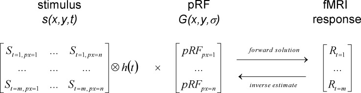
The components of the pRF linear model. The input stimulus and the pRF are represented as matrices, where vertical and horizontal space are collapsed into a single dimension (px = 1…n) and time is the other dimension (t = 1…m).

We modeled the hemodynamic response function as a gamma function h(t):

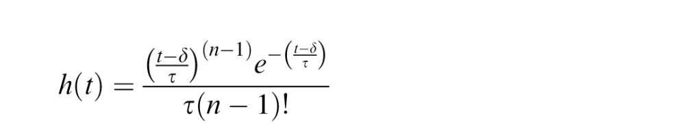with parameters n = 3, τ = 1.5 s, and δ = 2.25 s (Boynton, Engel, Glover, & Heeger, 1996).

We refer to the process of generating the predicted fMRI response, given the input stimulus and the pRF parameters, as the forward solution (rightward arrow in Figure 2). The inverse estimate is the process of finding the pRF parameters that, given the input stimulus, maximize the correspondence between the predicted and the observed fMRI response (leftward arrow in Figure 2).

To obtain pRF estimates, we first used the forward solution to generate the predicted fMRI response for a large set of initial pRF parameters (Gx and Gy values between −10° and +10° in steps of 1°, and Gσ between 1° and 10° in steps of 2°). For each voxel, we measured the correlation (our goodness-of-fit index) between the predicted and observed fMRI responses. The parameters yielding the highest correlation were used to initialize a nonlinear search procedure (Matlab simplex algorithm), which manipulated Gx, Gy, and Gσ to maximize goodness of fit. The initialization process allowed us to shorten search time, reduced the impact of local minima, and excluded voxels with weak response modulation (for which the correlation with the initialization parameters was lower than 0.2; under the assumption of linearity, this corresponds to a R² of 0.04).

Some minor modifications of our procedure relative to that described by Dumoulin and Wandell (2008) are the following: (a) we maximized the correlation between the predicted and observed fMRI response time-courses rather than minimizing the root mean square error; this eliminates the need to estimate a scale factor to account for the unknown units of the BOLD (Blood Oxygenation Level Dependent) signal; (b) we used a canonical hemodynamic response function rather than one estimated from the dataset.

The pRF fit was deemed unsuccessful if: (a) it failed the initialization procedure or it did not converge; (b) it provided unrealistic estimates of eccentricity (>16°, twice the maximum stimulated eccentricity) or sigma (<0.1°, limited by the 0.25° resolution at which the visual stimulus was rendered); or (c) the goodness of fit was <0.4. Data collected with the two stimulation sequences (multifocal and drifting bars) and in the two conditions (full-field and scotoma) were fit separately, yielding four independent sets of pRF estimates. For the full-field condition, pRFs were estimated with the input stimulus (the matrix representing the pattern of visual stimulation over time) representing the actual full-field visual stimulus. For the scotoma condition, we considered two possibilities. In the first analysis, the input represented the full-field stimulus, even though the actual visual stimulus was masked in the scotoma area. We refer to this approach as the “full-stimulus pRF method.” This method has been used in previous studies to investigate the effects of a simulated scotoma (Baseler et al., 2011; Haak et al., 2012). In the second analysis, we incorporated the scotoma into the input stimulus (the “effective-stimulus pRF method”). Note that in all cases (full-stimulus and effective-stimulus pRF methods), the fixation area (eccentricity <1°) was represented as unstimulated. Part of this area actually contained visual stimulation (the colored quadrants of the Simon© game), but this is expected to produce very little if any modulation of fMRI activity because the pace of stimulation was controlled by the subject, was not synchronized with the fMRI pulses (TR), and was fast, with very short temporal separation between identical repetitions.

We estimated the expected biases in pRF estimates obtained using the full-stimulus pRF method to analyze data from the scotoma condition in the following way. First, we used the forward solution and the pRFs estimated from the full-field condition, to simulate fMRI time-courses for the scotoma condition. We then estimated a new set of pRFs from these simulated fMRI responses using the full-stimulus pRF method. This produced an estimate of the biases in pRF estimates that we should expect from using a full-field stimulus as input into the pRF model when the stimulus contained a scotoma. These simulations had no free parameters, no noise was added, and used the actual pattern of stimulation presented in the fMRI experiments, with separate simulations for the multifocal and drifting bars sequences. We then showed that the magnitude and direction of these biases are consistent with pRFs estimated obtained using the full-stimulus pRF method from the actual measured fMRI responses in the scotoma condition.

The sets of pRFs obtained in the different conditions, measured and simulated, were compared in terms of goodness of fit, pRF size (Gσ), and pRF eccentricity; the latter was computed by transforming the Cartesian coordinates of the pRF center (Gx and Gy) into polar coordinates (eccentricity and polar angle). Because the distributions of pRF eccentricity, size and goodness of fit were nonnormal (Lilliefors test, p < 0.001), the median was preferred over the mean as a summary statistics, and statistical comparisons adopted a nonparametrical approach.

Results

We measured fMRI responses to randomized multifocal patches and drifting bars under two conditions. In the full-field condition, the stimulus covered the entire display region (Figure 1A, B); in the scotoma condition the central 2° were masked (Figure 1C, D). We estimated the parameters of pRFs (Dumoulin & Wandell, 2008) for voxels in a large bilateral occipital ROI (blue outline in Figure 3A, B, and E) within which three subregions were defined, corresponding to areas V1–V3 (black outlines).

pRFs in the full-field condition

The color shading in Figure 3A and B represents the goodness of fit of pRF estimates obtained in the full-field condition with the two stimulation sequences. Only voxels for which a pRF was successfully fit are mapped (see Methods for the criteria defining a successful fit; these include goodness of fit >0.4—under the assumption of linearity, this corresponds to R² = 0.16, similar to the R² > 0.15 inclusion criterion used in previous studies; Baseler et al., 2011).

For all analyses we pooled data across subjects after having verified that a similar pattern of results was obtained for individual subjects. For Figure 3C and D and Figure 7, analyses were restricted to voxels located in the three subregions of interest V1–V3. The bar-plots in Figure 3C and D show the proportion of voxels that were successfully fit in V1–V3 for the two stimulus sequences (stacked barplot with colored bands specifying the distribution of goodness-of-fit indices). Across ROIs, goodness-of-fit values were higher when using the drifting bars sequence than the multifocal sequence (Mann-Whitney U-tests, null hypothesis: median goodness of fit equal across stimulus types, p < 10⁻¹⁰ for V1–V3). For the multifocal stimulus sequence, successfully fit pRFs clustered in V1–V3 (83%), consistent with the pattern of responses known to be evoked by this stimulus (Vanni et al., 2005). For the drifting bars stimulus, a substantial proportion of successfully fit pRFs (44%) were distributed on the lateral face of the occipital lobe in areas beyond V1–V3.

Figure 7.

Comparison of predicted and observed pRFs shifts across ROIs. Bar graphs adopt the same format as the inset in Figure 6A and B, showing the median eccentricity difference between pRF eccentricity in the scotoma and full-field conditions (voxels with full-field pRFs between 1.5° and 2.5°), for the simulations and the pRF estimates obtained with the full-stimulus pRF method. For each ROI, parentheses give the number of voxels included in the analysis in each ROI and for each stimulus sequence (this is different than in Figures 4 and 6, where the sample of analyzed voxels was the same for the two stimulus sequences).

For Figures 3E and F, 4, and 6, analyses included all voxels successfully fit using both stimulus sequences in the full-field condition. These are shown in Figure 3E (for one exemplificative subject) and included approximately 500 voxels per subject, primarily distributed across all three V1–V3 ROIs (44% in V1, 23% in V2, 17% in V3; the remaining 16% was outside these areas). Figure 3F shows the distribution of goodness-of-fit values for pRFs estimated with the two stimulation sequences. Values are higher for the drifting bars sequence, suggesting that this allowed for more reliable pRF estimates in the selected set of voxels. The larger number of data-points (TRs) acquired for the drifting bars sequence may partially account for this result—but a direct comparison is difficult, since the TR duration was also different across sequences.

Figure 4 compares the parameters of pRFs estimated in the full-field condition, using the multifocal and the drifting bars stimulation sequences. As in Figure 3E and F, analyses were restricted to voxels successfully fit using both stimulus sequences in the full-field condition. The relationship between pRF size and eccentricity is shown for the central 4° of visual space (covered by both stimulation sequences). In this range, pRF size grows with eccentricity and the trends are adequately fit by linear functions, consistent with previous studies (Dumoulin & Wandell, 2008). The best-fitting linear functions have comparable slopes (linear fit with SEM as weights; multifocal sequence: adjusted R² = 0.82, slope = 0.14 ± 0.02; drifting bars sequence: adjusted R² = 0.74, slope = 0.20 ± 0.04). However, the linear fit for the multifocal sequence yields a smaller intercept (multifocal sequence: intercept = 0.36° ± 0.05°; drifting bars sequence: intercept = 0.53° ± 0.1°)—pRFs estimated using the multifocal sequence tended to be smaller than those estimated with the drifting bars sequence.

Figure 4.

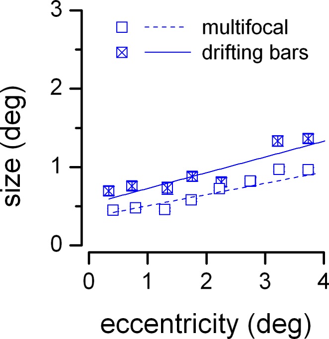
pRFs in the full-field condition for the multifocal and the drifting bars stimulation sequences. pRF size is plotted against pRF eccentricity; voxels are binned in contiguous 0.5° steps. Symbols show medians in each bin for the two stimulus sequences. Continuous lines are linear fits through the data points in each series, weighted by the inverse of their SEM (error bars, smaller than symbol size). This analysis included all voxels successfully fit using both the multifocal and the drifting bars sequence.

pRFs in the scotoma condition: Simulations and results

Figure 5 illustrates a key notion: pRF parameters can be accurately estimated only if the stimulus generating the fMRI response and the stimulus representation used for pRF fitting match. If they don't match, pRF estimates are biased.

Figure 5.

Schematic illustration of our simulations. pRFs estimated from the full-field condition (three examples in panels A–C, top) and the stimulus sequence from the scotoma condition were entered in the “forward solution” to obtain simulated fMRI responses (black lines and circles). For the purpose of this illustration, the time dimension is ignored; stimulus and response are plotted as a function of eccentricity. Two methods were then used to recover the pRF parameters from the simulated fMRI responses: the full-stimulus pRF method, where the full-field stimulus was used as input to the pRF fitting procedure, and the effective-stimulus pRF method, where the scotoma is modeled in the stimulus representation. The bottom rows show the recovered pRFs with the two methods (red and green, respectively) together with the original pRFs (blue).

Assuming that the pRF of a voxel is known (blue lines in Figure 5), its fMRI response to a given stimulation sequence can be generated by multiplying the stimulus with the pRF, then convolving by the hemodynamic response function (the forward solution, see Methods, black lines and circles in Figure 5). This simulated fMRI response can be used, like a real fMRI time-course, to estimate the pRF parameters of the voxel—using the inverse estimate, which simply searches for the pRF that, multiplied with the stimulus sequence and convolved by the hemodynamic response function, best predicts the voxel fMRI response.

The red lines in Figure 5 illustrate the case where the fMRI response is generated using a stimulus with a foveal scotoma (gray area), but the pRF fitting is performed assuming a stimulus covering the full visual field. We term this procedure the “full-stimulus pRF method” (Baseler et al., 2011; Haak et al., 2012). The green lines show estimated pRFs when the fitting is performed assuming a stimulus that accounts for the foveal scotoma, thereby matching the stimulus used to generate the fMRI responses. We term this procedure the “effective-stimulus pRF method.”

When using the full-stimulus pRF method, pRF estimates are biased. Different voxels show different kinds of artifacts. Small pRFs that do not span the scotoma (Figure 5A) shrink and shift away from the scotoma region. PRFs that span the scotoma (small pRFs located at the center of the scotoma as in Figure 5B, or large pRFs located near the edges of the scotoma as in Figure 5C) do not shift but are enlarged. Given a fixed distance of the pRF from the scotoma center (e.g., 1° as in Panels A and C), large pRFs shift less than small pRFs (i.e., there is a large shift for the pRF in Panel A and a very small shift for the pRF in Panel C)—this effect of pRF size is discussed in more detail below and in Supplementary Figure S1 as it explains the difference in magenta lines in Figure 6A versus B.

Figure 6.

Comparison of pRFs from the full-field and the scotoma condition. Separate panels show results for the multifocal (A and C) and drifting bars stimulus sequence (B and D). The gray shadow represents the scotoma region. Panels A and B plot the eccentricity of pRFs from the scotoma condition against the eccentricity of pRFs from the full-field condition. Inset bar graphs show the median eccentricity difference between pRF eccentricity in the scotoma and full-field conditions (voxels with full-field pRFs between 1.5° and 2.5°; ***p < 0.001). Panels C and D plot the size of pRFs obtained in each condition and with each analysis method against the respective eccentricity. Voxels were pooled across subjects and binned into contiguous 0.5° bins; symbols report medians in each bin and error bars show SEM.

In contrast, using the effective-stimulus pRF method allows for obtaining accurate pRF estimates in all cases (i.e., the green lines match the “true pRFs” in all panels of Figure 5).

We used both the full-stimulus pRF method and the effective-stimulus pRF method to estimate pRFs from the fMRI responses observed in our scotoma condition; the resulting parameters are plotted in Figure 6 as red and green symbols, respectively (blue symbols show pRF parameters estimated in the full-field condition).

We also performed quantitative simulations following the logic of Figure 5. As described in the Methods section, we started from the actual distribution of pRFs estimated in the full-field condition, separately for the multifocal and drifting bars stimulus sequences. We then generated simulated responses for all voxels by multiplying the full-field pRFs with the scotoma stimulus (the multifocal and drifting bars stimulus sequences, with the central 2° masked). Finally, we re-estimated the pRF parameters with the full-stimulus pRF method and quantified how they differed from the original pRFs. These estimates (shown in magenta in Figure 6) provided quantitative predictions of the pattern of biases expected from using the full-stimulus pRF method to estimate pRFs for the scotoma condition.

Figure 6A and B plots the eccentricity of pRFs in the scotoma condition against the eccentricity of pRFs in the full-field condition, for the multifocal (Panel A) and drifting bars stimulus sequences (Panel B). Unbiased pRF estimates would result in data points distributed along the y = x line. Red lines and symbols show the pRF parameters estimated from (real) fMRI responses from the scotoma condition using the full-stimulus pRF method. pRF estimates are biased, shifted away from the scotoma edges (the gray shaded area), like in the cartoon illustration of Figure 5. These biases cannot be explained by changes in the voxel's response properties, for two reasons: (a) because they are largely predicted by our simulations (magenta) and (b), because analyzing the same (real) fMRI data with the effective-stimulus pRF method (green) resulted in virtually veridical estimates.

Two features in the results in Figure 6A and B merit particular attention.

First, the pattern of predicted biases is different for the multifocal and the drifting bars sequence (compare the magenta lines in Figure 6A vs. B). This is because larger pRF sizes were estimated in the full-field condition for the drifting bars stimulus than for the multifocal stimulus (Figure 4). Larger pRFs are less biased than small pRFs near the edges of the scotoma (as illustrated in Figure 5); however, they are more biased in flanking regions (Supplementary Figure S1). Thus, one should not conclude that larger pRFs (such as those produced by the drifting bars sequence) are less susceptible to biases in the presence of a scotoma.

Second, while the general pattern of results obtained with both our stimulus sequences showed a remarkable correspondence with our simulations, the results from the drifting bars sequence were less consistent with our predictions than those from the multifocal sequence (the red curve is different from the magenta curve in Figure 6B while the two are well matched in Figure 6A). This is best appreciated in the inset bar graphs in Figure 6A and B, which show the median bias (the eccentricity difference between the estimates of pRF eccentricity for the scotoma condition and the full-field condition) across voxels located in the proximity of the scotoma edge (1° interval). For the multifocal sequence, the bias of pRF estimates obtained with the full-stimulus pRF method is significant (Wilcoxon signed rank test, null hypothesis: red bar = 0, p < 0.001, n = 288) and virtually indistinguishable from the bias predicted from our stimulations (Mann-Whitney U test, null hypothesis: red bar = magenta bar, p = 0.4), while estimates obtained with the effective-stimulus pRF method are accurate (Wilcoxon signed rank test, null hypothesis: green bar = 0, p = 0.25). In contrast, for the drifting bars sequence, the observed bias is significantly smaller than that predicted from our stimulations (Mann-Whitney U test, null hypothesis: red bar = magenta bar, p < 0.001, n = 226), although still significantly larger than zero (Wilcoxon signed rank test, null hypothesis: red bar = 0, p < 0.001), and the effective-stimulus pRF method produced a slight bias in the opposite direction, i.e., towards the center of the scotoma (Wilcoxon signed rank test, null hypothesis: green bar = 0, p = 0.018).

Figure 6C and D plots the estimated size of pRFs from the full-field and scotoma conditions, as a function of their respective eccentricity estimates (pRFs from the full-field condition are replotted from Figure 4A). As illustrated in Figure 5, our simulations predicted that the pattern of biases for pRF size estimates depends on pRF eccentricity, such that pRFs near the scotoma edges shrink and pRFs near the scotoma center enlarge. For the multifocal sequence, estimates obtained with the full-stimulus pRF method (red) followed this pattern; biases were closely matched by our quantitative predictions (magenta), and the effective-stimulus pRF method (green) improved the accuracy of pRF size estimates. For the drifting bars sequence, the predictions from our simulations did not match the results of the full-stimulus pRF method as closely, and there was little difference in the accuracy of estimates obtained with the full-stimulus pRF method and the effective-stimulus pRF method.

We repeated this analysis with different voxel selection criteria and verified that the results were not qualitatively altered. In addition, Figure 7 shows the results of an ROI-based analysis of the pRF shifts in the scotoma condition; for this analysis, the number of pRFs was not necessarily matched for the multifocal and drifting bars sequences (contrary to Figures 4 and 6). The bar plots show the median bias (the eccentricity difference between the estimates of pRF eccentricity for the scotoma condition and the full-field condition) across voxels located in the proximity of the scotoma edge (1° interval, equivalent to the inset plots of Figure 6A, B). The bias of pRF estimates obtained with the full-stimulus pRF method is very close to the bias predicted from our stimulations for the multifocal sequence, whereas the observed bias is consistently smaller than that predicted from our stimulations for the drifting bars sequence—the same pattern of results obtained in the main analysis of Figure 6. A Friedman test confirms that the effect of stimulus type (multifocal vs. drifting bars) is statistically reliable (dependent variable: difference between observed and simulated bias; the test assesses the effect of the primary factor, stimulus type, after taking into account variability across a secondary factor, ROI; df: 1; Chi-square value: 11.59; p < 0.001; because the test requires a constant number of observations in all cells, the statistics were computed for the 69 most reliable voxels in all ROIs).

Discussion

In summary, we estimated the location and size of pRFs in the early visual cortex using two stimulus sequences (multifocal patches and drifting bars) covering a large part of the central visual field. We then used these pRF estimates to generate simulated fMRI response time-courses to the stimulus used in the scotoma condition (i.e., the full-field condition, with a mask covering the central 2° mimicking a foveal scotoma). A crucial step in the pRF estimation process is the definition of a space-time matrix describing the pattern of visual stimulation over time. In the full-stimulus pRF method, this space-time matrix describes the stimulus of the full-field condition, irrespective of any scotoma. Analyzing the simulated fMRI time-courses with this method resulted in pRFs that were shifted in position and changed in size. This is a consequence of failing to model the absence of visual stimulation in part of the visual field. We then measured actual fMRI response time-courses in the scotoma condition, and compared the pRFs obtained from analyzing actual responses with the full-stimulus pRF method to the results of our simulations. We also analyzed fMRI responses with an effective-stimulus pRF method, where the space-time matrix describing the stimulus for pRF fitting is a more accurate representation of the visual input effectively driving fMRI responses (in our case, the stimulus with a mask covering the central 2°). For data collected with the multifocal stimulus sequence, the full-stimulus pRF method resulted in pRF changes that matched those predicted by our simulations, and pRFs estimated with the effective-stimulus method were unbiased, i.e., unaffected by the presence of the scotoma. Thus, in this case, pRF shifts and size changes obtained using the full-stimulus pRF method are purely an artifact, and do not imply any reorganization of the voxel response properties.

It is important to note that the retinotopic mapping artifact predicted by our simulations is not specific to the pRF method. Analogous biases would be produced by phase-encoded retinotopic mapping methods (Engel et al., 1994). For example, when an expanding ring is partially masked by a foveal scotoma, the very same logic at the basis of our simulations predicts a delay in the response of voxels located near the scotoma edges, resulting in these voxels being assigned to more peripheral locations. However, modeling the absence of visual input in the scotoma area is not possible with the phase-encoded method, due to its reliance on the periodicity of the stimulation sequence. Here we show that an added value of the pRF method is that it can easily account for the absence of visual input in the scotoma area (the effective-stimulus method), allowing for unbiased retinotopic mapping estimates.

pRF estimates using drifting bars versus multifocal sequences

There were several differences between the pRF parameters estimated in the full-field condition using the multifocal and the drifting bars stimulus. In particular, pRF sizes were larger for the drifting bars sequence than the multifocal sequence (Figure 4). One possible explanation for this is that high spatial frequencies were slightly more represented in the multifocal stimulus sequence (see Fourier spectra in Supplementary Figure S2), thereby recruiting a higher proportion of neurons with small receptive fields. This explanation might also account for the higher number of pRFs successfully fit with the multifocal sequence in early visual areas compared to areas beyond V3, where neurons with small receptive are less represented.

This pRF size difference had a prominent effect on the pattern of biases predicted to occur when analyzing data from the scotoma condition with the full-stimulus method (predictions derived from simulations: magenta lines in Figure 6A vs. B), and is the reason why predicted biases were smaller for the drifting bars sequence than for the multifocal sequence. As described in Figure 5 and detailed in Supplementary Figure S1, the pattern of expected biases depends both on the distance of the pRF from the scotoma and the relative sizes of the pRF and the scotoma. Larger pRFs are less biased near the center of the scotoma, but more biased at flanking locations compared to smaller pRFs. Therefore, the results of our simulations do not indicate that larger pRFs (such as pRFs estimated using the drifting bars stimulus) are less susceptible to scotoma-induced biases.

Besides this difference in the simulated pattern of biases between multifocal and drifting bars sequences, there was an unexpected difference between the measured and the simulated patterns of bias for the drifting bars sequence: pRFs estimated with the drifting bars sequence were less biased than predicted by our simulations, and biases were therefore over-corrected when using the effective-stimulus pRF method. This result cannot be explained by differences in the pRF sizes estimated in the full-field conditions (which are taken into account in the simulations). Rather, this result implies that fMRI activity is affected by factors other than the pattern of visual stimulation—violating one of the fundamental assumptions of retinotopic mapping methods. More specifically, we speculate that the pattern of results obtained for the drifting bars sequence might be caused by fMRI responses being generated in nondirectly stimulated voxels. These can be produced by at least three phenomena: (a) optical blur, (b) nonlinear interactions between BOLD responses in neighboring voxels over time, and (c) neural responses related to the predictability of the stimulation sequence. These last two factors would be expected to differentially affect responses to the multifocal and drifting bars sequence.

As far as spatio-temporal interactions are concerned, previous work has shown that spatial and temporal summation of BOLD signals are well approximated by the linear model; however, examples of nonlinear interactions have been reported (Zenger-Landolt & Heeger, 2003; Pihlaja, Henriksson, James, & Vanni, 2008). It is possible that that responses to coherently moving stimuli, generating a “traveling wave” of activity across the cortical surface (Engel et al., 1994), are stronger and spread across a larger area of cortex than responses to randomized sequences. Stronger responses (implying enhanced signal to noise ratio) might explain why pRF estimates showed higher reliability for the drifting bars sequence than for the multifocal sequence. The spread of BOLD signals across neighboring voxels would produce a pattern of fMRI responses consistent with a larger stimulus bar, which might explain why pRF size estimates were larger for the drifting bars sequence (though, as noted above, size differences may also be explained by the different spatial frequency content of the two stimuli). Finally, if BOLD signals spread to voxels representing the scotoma region, the resulting pattern of fMRI responses might be akin to that elicited by a smaller scotoma. This might explain why, for the drifting bars stimulus, pRFs estimated from the scotoma condition were less biased than predicted from our simulations.

As far as stimulus predictability is concerned, this might have affected the response to the drifting bars stimulus in two ways. First, previous attentional studies have suggested that fMRI responses are affected by expectations about the upcoming pattern of stimulation (Kastner, Pinsk, De Weerd, Desimone, & Ungerleider, 1999). Perhaps, despite subjects being engaged in a demanding task at fixation, some fMRI activity was induced at the upcoming locations of the predictable drifting bars stimulus. Second, our stimulus might easily be interpreted as a partially occluded object—the bar passing behind the simulated scotoma—thereby generating fMRI responses within the scotoma. Such fill-in phenomena have been shown to occur automatically and independently of the location of attention (Meng, Remus, & Tong, 2005).

Only the multifocal sequence resulted in pRF biases that could be entirely explained and corrected by our linear model. The systematic deviations between model predictions and the observed biases for the drifting bar stimulus implies that the pRF model does not provide an adequate model for responses to the drifting bars stimulus. The fact that the failure of the model was in the direction of showing less bias than predicted is not a desirable feature, especially while the cause of this undershoot in not fully understood. For example, if the undershoot is due to nonneural activity, then using a drifting bars sequence would result in underestimating actual pRF shifts in a hypothetical case of cortical reorganization. If this undershoot is due to predictive responses from higher visual areas, then comparing multifocal and drifting bars stimuli might provide a way of separately measuring bottom-up and top-down responses.

Despite this advantage (results are explained by the linear pRF model), it should be noted that the multifocal sequence does have some clear disadvantages relative to more conventional stimulus sequences (e.g., the drifting bars). In particular, the multifocal stimulus only allows for pRF estimation in a subset of visual areas, essentially restricted to areas V1–V3. Even in these early visual areas, goodness-of-fit values were lower for the multifocal stimulus, suggesting that for many purposes (e.g., retinotopic mapping to identify visual areas in individuals without visual loss) more traditional stimuli may be preferable, as they afford better signal to noise ratio.

Comparison with previous studies

Two previous studies have investigated the effects of foveal scotomas on pRF estimates; both used non-random stimulation sequences and reported large pRF shifts away from the scotoma edges (Baseler et al., 2011; Haak et al., 2012). Since their estimates were mainly obtained using the full-stimulus pRF method it is likely that these shifts are at least partially artifactual. However, one of the analyses in Haak et al. (2012) adopted an approach similar to our effective-stimulus pRF method and still found large pRF shifts away from the scotoma (i.e., an effect opposite to that observed here with the drifting bars sequence, where the effective-stimulus pRF method over-corrected the pRF shifts). There are a number of differences between their experiments and ours that might explain these findings. The stimulus sequences are different in several respects: These studies employed a ring stimulus moving in a single direction (expansion) and appearing from behind a large scotoma (5°–7° in Haak et al.'s study), whereas our bar drifted in random directions past a small (2°) scotoma. As discussed above, the effects of spatio-temporal nonlinearities, expectations and fill-in are all likely to be heavily affected by the type of stimulus sequence. The size of the simulated scotoma might also be important. An assumption of the pRF method is that the underlying aggregate of neural receptive fields is accurately represented by a Gaussian distribution. Under the conditions of our study, we found no indication that the Gaussian model is substantially inaccurate. However, deviations from the Gaussian model might be more pronounced at the larger eccentricities tested by Haak et al. study. If the underlying neural population has heavier tails then a Gaussian function, then the pRF shifts induced by a scotoma would be larger than accounted for by the effective-stimulus pRF method—this argument echoes Haak et al.'s suggestion of different statistics of the neural population contributing to the voxel activity with and without the scotoma. Finally, subjects were tested in passive viewing in Haak et al.'s study, whereas they performed a fixation task in our study, and there is evidence to suggest that attention modulates responses in nondirectly stimulated voxels located within a scotoma (Masuda et al., 2008).

Haak et al. (2012) suggested that changes in pRF estimates could result from an altered balance between the direct visual input to the center of the neural receptive fields and feedback signals to the receptive field surround, possibly subtending fill-in phenomena. For the sake of clarity, we note that while both we and these authors call into play fill-in, the two arguments are used to explain pRF shifts in opposite directions and might describe different aspects of the phenomenon. Baseler et al. (2011) and Haak et al. (2012) suggest that fill-in might shift the neural receptive field away from the scotoma edges. Conversely, having shown that pRF shifts away from the scotoma edges can be expected as a result of artifacts of the full-stimulus pRF method, we suggest that fill-in might result in induced neural signals within the scotoma that reduce the size of the effective scotoma and results in pRFs shifts being smaller than expected.

Implications for measuring retinotopic maps after partial visual loss

In our experiments, we simulated an unrealistically regular pattern of visual loss, a foveal scotoma with fixed location and size and sharp edges. This allowed us to exactly describe the effective retinal input generating the fMRI responses, which was entered the pRF fitting procedure to eliminate a major source of artifacts in pRF estimates. However, this procedure can be extended to more complicated and realistic patterns of visual loss, including scotomas with gradual borders. The Appendix describes how the spatial profile of the visual impairment measured by psychophysical techniques (e.g., the Humphrey Field Analyzer II, Carl Zeiss Meditec, Dublin, CA) can be used to modify the stimulus representation entered the pRF fitting procedure.

An accurate representation of the effective visual input should minimize biases in pRF estimates irrespective of the site of visual dysfunction, be it retinal, of the optic pathway, or cortical. However, modeling the effective visual input following cortical damage presents further difficulties. For example, while a focal V1 lesion would be likely to affect the input to more central extra-striate areas (e.g., V2–V3), it may have little or no effect on the input to neighboring V1 regions. In these cases, the choice of the stimulus representation (the effective stimulus, reflecting either the physically displayed stimulus or the display weighted by the subject's contrast sensitivity) would need to be based on prior knowledge on the relationship between the visual loss and activity in the cortical areas of interest.

Conclusions

We have shown that a large artifact in retinotopic mapping estimates can be expected for early visual cortex voxels that are located within or near the edges of a scotoma. When using a random multifocal stimulus sequence, this artifact can be eliminated using a modification of the pRF method, which simply requires entering the pRF fitting procedure with a representation of the effective visual stimulus (the full-field stimulus, masked by the scotoma). With non-random stimulus sequences, like drifting bars, the pattern of results is more complex, and additional factors such as spatio-temporal nonlinearities, expectation, and neural fill-in may significantly affect responses. We conclude that accurately measuring retinotopic maps under conditions of partial visual loss requires both a modeling method that takes into account the pattern of visual loss and an appropriate stimulus sequence.

Appendix

Visual losses can be taken into account in the pRF method by modulating the binary values describing the spatiotemporal pattern of stimulation s(x, y, t) according to the spatial profile of the visual impairment. This can be done by weighting the physical stimulus (e.g., the stimulus presented in the full-field condition of our experiments) by the patient's visual sensitivity at each location, as estimated in a perimetry test (e.g., the Humphrey Field Analyzer II, Carl Zeiss Meditec, Dublin, CA). Here we describe the weighting based on “pattern deviation” (pd), a measure of sensitivity used by the Humphrey's Static Threshold tests. This measure describes the visual impairment at each location in the visual field, irrespectively of overall sensitivity losses (e.g., caused by cloudy media or cataracts). The units are decibels, such that a pattern deviation of zero decibels implies no sensitivity loss and pattern deviation of two decibels implies a 100-fold sensitivity loss.

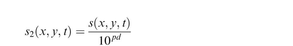Given that the stimulus is now effectively grayscale and BOLD responses to contrast are known to be nonlinear, a nonlinear contrast response function should also be included, such that

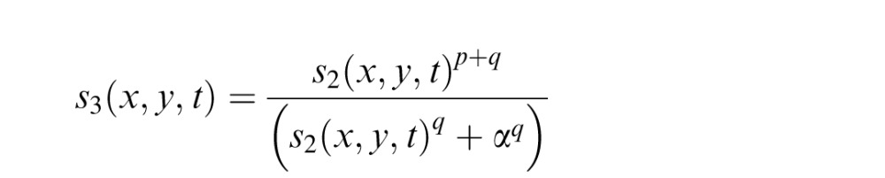where p, q, and α determine the shape of the contrast–response function. When s₂(x, y, t) > > α, the function behaves like a simple power function with an exponent of p. When s₂(x, y, t) < < α, the function behaves like a power function with an exponent of p + q. Typical values of p and q are 0.3 and 2, respectively, so that the function is expansive at low contrasts and compressive at high contrasts. Depending on the level of precision that is desired, these parameters p, q, and α can be estimated either by using canonical values from the literature (Boynton, Demb, Glover, & Heeger, 1999; Olman, Ugurbil, Schrater, & Kersten, 2004), or they can be explicitly estimated by measuring the contrast response function across voxels (in a separate scan or by including contrast modulations of the retinotopic mapping stimulus in regions of the visual field that are unimpaired).

Once these computations are performed, the pRF estimation method proceeds in the same way as for subjects with normal vision (see Methods), except that the stimulus matrix s(x, y, t) is replaced with the s₃(x, y, t) matrix defined above.

References

- Baker C. I., Dilks D. D., Peli E., Kanwisher N. (2008). Reorganization of visual processing in macular degeneration: Replication and clues about the role of foveal loss. Vision Research, 48 (18), 1910–1919, http://www.ncbi.nlm.nih.gov/entrez/query.fcgi?cmd=Retrieve&db=PubMed&dopt=Citation&list_uids=18620725 [DOI] [PMC free article] [PubMed] [Google Scholar]
- Baker C. I., Peli E., Knouf N., Kanwisher N. G. (2005). Reorganization of visual processing in macular degeneration. Journal of Neuroscience, 25 (3), 614–618, http://www.ncbi.nlm.nih.gov/entrez/query.fcgi?cmd=Retrieve&db=PubMed&dopt=Citation&list_uids=15659597 [DOI] [PMC free article] [PubMed] [Google Scholar]
- Barton B., Brewer A. (2011). FMRI of the rod scotoma: Cortical projections, filling-in and insights into plasticity. Journal of Vision, 11 (15): 9, http://www.journalofvision.org/content/11/15/9, doi:10.1167/11.15.9. [Abstract] [Google Scholar]
- Baseler H. A., Brewer A. A., Sharpe L. T., Morland A. B., Jagle H., Wandell B. A. (2002). Reorganization of human cortical maps caused by inherited photoreceptor abnormalities. Nature Neuroscience, 5 (4), 364–370, http://www.ncbi.nlm.nih.gov/entrez/query.fcgi?cmd=Retrieve&db=PubMed&dopt=Citation&list_uids=11914722 [DOI] [PubMed] [Google Scholar]
- Baseler H. A., Gouws A., Haak K. V., Racey C., Crossland M. D., Tufail A., et al. (2011). Large-scale remapping of visual cortex is absent in adult humans with macular degeneration. Nature Neuroscience, 14 (5), 649–655, http://www.ncbi.nlm.nih.gov/entrez/query.fcgi?cmd=Retrieve&db=PubMed&dopt=Citation&list_uids=21441924 [DOI] [PubMed] [Google Scholar]
- Baseler H. A., Morland A. B., Wandell B. A. (1999). Topographic organization of human visual areas in the absence of input from primary cortex. Journal of Neuroscience, 19 (7), 2619–2627, http://www.ncbi.nlm.nih.gov/entrez/query.fcgi?cmd=Retrieve&db=PubMed&dopt=Citation&list_uids=10087075 [DOI] [PMC free article] [PubMed] [Google Scholar]
- Boynton G. M., Demb J. B., Glover G. H., Heeger D. J. (1999). Neuronal basis of contrast discrimination. Vision Research, 39 (2), 257–269, http://www.ncbi.nlm.nih.gov/entrez/query.fcgi?cmd=Retrieve&db=PubMed&dopt=Citation&list_uids=10326134 [DOI] [PubMed] [Google Scholar]
- Boynton G. M., Engel S. A., Glover G. H., Heeger D. J. (1996). Linear systems analysis of functional magnetic resonance imaging in human V1. Journal of Neuroscience, 16 (13), 4207–4221, http://www.ncbi.nlm.nih.gov/entrez/query.fcgi?cmd=Retrieve&db=PubMed&dopt=Citation&list_uids=8753882 [DOI] [PMC free article] [PubMed] [Google Scholar]
- Brainard D. H. (1997). The Psychophysics Toolbox. Spatial Vision, 10 (4), 433–436, http://www.ncbi.nlm.nih.gov/entrez/query.fcgi?cmd=Retrieve&db=PubMed&dopt=Citation&list_uids=9176952 [PubMed] [Google Scholar]
- Dilks D. D., Baker C. I., Peli E., Kanwisher N. (2009). Reorganization of visual processing in macular degeneration is not specific to the “preferred retinal locus.” Journal of Neuroscience, 29 (9), 2768–2773, http://www.ncbi.nlm.nih.gov/entrez/query.fcgi?cmd=Retrieve&db=PubMed&dopt=Citation&list_uids=19261872 [DOI] [PMC free article] [PubMed] [Google Scholar]
- Dilks D. D., Serences J. T., Rosenau B. J., Yantis S., McCloskey M. (2007). Human adult cortical reorganization and consequent visual distortion. Journal of Neuroscience, 27 (36), 9585–9594, http://www.ncbi.nlm.nih.gov/entrez/query.fcgi?cmd=Retrieve&db=PubMed&dopt=Citation&list_uids=17804619 [DOI] [PMC free article] [PubMed] [Google Scholar]
- Dumoulin S. O., Wandell B. A. (2008). Population receptive field estimates in human visual cortex. Neuroimage, 39 (2), 647–660, http://www.ncbi.nlm.nih.gov/entrez/query.fcgi?cmd=Retrieve&db=PubMed&dopt=Citation&list_uids=17977024 [DOI] [PMC free article] [PubMed] [Google Scholar]
- Engel S. A., Rumelhart D. E., Wandell B. A., Lee A. T., Glover G. H., Chichilnisky E. J., et al. (1994). fMRI of human visual cortex. Nature, 369 (6481), 525, http://www.ncbi.nlm.nih.gov/entrez/query.fcgi?cmd=Retrieve&db=PubMed&dopt=Citation&list_uids=8031403 [DOI] [PubMed] [Google Scholar]
- Haak K. V., Cornelissen F. W., Morland A. B. (2012). Population receptive field dynamics in human visual cortex. PLoS One, 7 (5), e37686, http://www.ncbi.nlm.nih.gov/entrez/query.fcgi?cmd=Retrieve&db=PubMed&dopt=Citation&list_uids=22649551 [DOI] [PMC free article] [PubMed] [Google Scholar]
- Hansen K. A., David S. V., Gallant J. L. (2004). Parametric reverse correlation reveals spatial linearity of retinotopic human V1 BOLD response. Neuroimage, 23 (1), 233–241, http://www.ncbi.nlm.nih.gov/entrez/query.fcgi?cmd=Retrieve&db=PubMed&dopt=Citation&list_uids=15325370 [DOI] [PubMed] [Google Scholar]
- Hoffmann M. B., Kaule F. R., Levin N., Masuda Y., Kumar A., Gottlob I., et al. (2012). Plasticity and stability of the visual system in human achiasma. Neuron, 75 (3), 393–401, http://www.ncbi.nlm.nih.gov/entrez/query.fcgi?cmd=Retrieve&db=PubMed&dopt=Citation&list_uids=22884323 [DOI] [PMC free article] [PubMed] [Google Scholar]
- Kastner S., Pinsk M. A., De Weerd P., Desimone R., Ungerleider L. G. (1999). Increased activity in human visual cortex during directed attention in the absence of visual stimulation. Neuron, 22 (4), 751–761, http://www.ncbi.nlm.nih.gov/entrez/query.fcgi?cmd=Retrieve&db=PubMed&dopt=Citation&list_uids=10230795 [DOI] [PubMed] [Google Scholar]
- Kriegeskorte N., Goebel R. (2001). An efficient algorithm for topologically correct segmentation of the cortical sheet in anatomical mr volumes. Neuroimage, 14 (2), 329–346, http://www.ncbi.nlm.nih.gov/entrez/query.fcgi?cmd=Retrieve&db=PubMed&dopt=Citation&list_uids=11467907 [DOI] [PubMed] [Google Scholar]
- Masuda Y., Dumoulin S. O., Nakadomari S., Wandell B. A. (2008). V1 projection zone signals in human macular degeneration depend on task, not stimulus. Cerebral Cortex, 18 (11), 2483–2493, http://www.ncbi.nlm.nih.gov/entrez/query.fcgi?cmd=Retrieve&db=PubMed&dopt=Citation&list_uids=18250083 [DOI] [PMC free article] [PubMed] [Google Scholar]
- Masuda Y., Horiguchi H., Dumoulin S. O., Furuta A., Miyauchi S., Nakadomari S., et al. (2010). Task-dependent V1 responses in human retinitis pigmentosa. Investigative Ophthalmology & Vision Science, 51 (10), 5356–5364, http://www.iovs.org/content/51/10/5356. http://www.ncbi.nlm.nih.gov/entrez/query.fcgi?cmd=Retrieve&db=PubMed&dopt=Citation&list_uids=20445118 [DOI] [PMC free article] [PubMed] [Google Scholar]
- Meng M., Remus D. A., Tong F. (2005). Filling-in of visual phantoms in the human brain. Nature Neurosci, 8 (9), 1248–1254, http://www.ncbi.nlm.nih.gov/entrez/query.fcgi?cmd=Retrieve&db=PubMed&dopt=Citation&list_uids=16116454 [DOI] [PMC free article] [PubMed] [Google Scholar]
- Morland A. B., Baseler H. A., Hoffmann M. B., Sharpe L. T., Wandell B. A. (2001). Abnormal retinotopic representations in human visual cortex revealed by fMRI. Acta Psychologica (Amst), 107 (1–3), 229–247, http://www.ncbi.nlm.nih.gov/entrez/query.fcgi?cmd=Retrieve&db=PubMed&dopt=Citation&list_uids=11388137 [DOI] [PubMed] [Google Scholar]
- Olman C. A., Ugurbil K., Schrater P., Kersten D. (2004). BOLD fMRI and psychophysical measurements of contrast response to broadband images. Vision Research, 44 (7), 669–683, http://www.ncbi.nlm.nih.gov/entrez/query.fcgi?cmd=Retrieve&db=PubMed&dopt=Citation&list_uids=14751552 [DOI] [PubMed] [Google Scholar]
- Pelli D. G. (1997). The VideoToolbox software for visual psychophysics: Transforming numbers into movies. Spatial Vision, 10 (4), 437–442, http://www.ncbi.nlm.nih.gov/entrez/query.fcgi?cmd=Retrieve&db=PubMed&dopt=Citation&list_uids=9176953 [PubMed] [Google Scholar]
- Pihlaja M., Henriksson L., James A. C., Vanni S. (2008). Quantitative multifocal fMRI shows active suppression in human V1. Human Brain Mapping, 29 (9), 1001–1014, http://www.ncbi.nlm.nih.gov/entrez/query.fcgi?cmd=Retrieve&db=PubMed&dopt=Citation&list_uids=18381768 [DOI] [PMC free article] [PubMed] [Google Scholar]
- Schmid M. C., Panagiotaropoulos T., Augath M. A., Logothetis N. K., Smirnakis S. M. (2009). Visually driven activation in macaque areas V2 and V3 without input from the primary visual cortex. PLoS One, 4 (5), e5527, http://www.ncbi.nlm.nih.gov/entrez/query.fcgi?cmd=Retrieve&db=PubMed&dopt=Citation&list_uids=19436733 [DOI] [PMC free article] [PubMed] [Google Scholar]
- Sunness J. S., Liu T., Yantis S. (2004). Retinotopic mapping of the visual cortex using functional magnetic resonance imaging in a patient with central scotomas from atrophic macular degeneration. Ophthalmology, 111 (8), 1595–1598, http://www.ncbi.nlm.nih.gov/entrez/query.fcgi?cmd=Retrieve&db=PubMed&dopt=Citation&list_uids=15288993 [DOI] [PubMed] [Google Scholar]
- Vanni S., Henriksson L., James A. C. (2005). Multifocal fMRI mapping of visual cortical areas. Neuroimage, 27 (1), 95–105, http://www.ncbi.nlm.nih.gov/entrez/query.fcgi?cmd=Retrieve&db=PubMed&dopt=Citation&list_uids=15936956 [DOI] [PubMed] [Google Scholar]
- Wandell B. A., Smirnakis S. M. (2009). Plasticity and stability of visual field maps in adult primary visual cortex. Nature Reviews Neuroscience, 10 (12), 873–884, http://www.ncbi.nlm.nih.gov/entrez/query.fcgi?cmd=Retrieve&db=PubMed&dopt=Citation&list_uids=19904279 [DOI] [PMC free article] [PubMed] [Google Scholar]
- Zenger-Landolt B., Heeger D. J. (2003). Response suppression in V1 agrees with psychophysics of surround masking. Journal of Neuroscience, 23 (17), 6884–6893, http://www.ncbi.nlm.nih.gov/entrez/query.fcgi?cmd=Retrieve&db=PubMed&dopt=Citation&list_uids=12890783 [DOI] [PMC free article] [PubMed] [Google Scholar]
- Zuiderbaan W., Harvey B. M., Dumoulin S. O. (2012). Modeling center-surround configurations in population receptive fields using fMRI. Journal of Vision, 12 (3): 10, 1–15, http://www.journalofvision.org/content/12/3/10, doi:10.1167/12.3.10. [PubMed] [Article] [DOI] [PubMed] [Google Scholar]