The neuroimaging signal is a linear sum of neurally distinct stimulus- and task-related components

Abstract

Neuroimaging (for example, functional magnetic resonance imaging) signals are taken as a uniform proxy for local neural activity. By simultaneously recording electrode and neuroimaging (intrinsic optical imaging) signals in alert, task-engaged macaque visual cortex, we recently observed a large anticipatory trial-related neuroimaging signal that was poorly related to local spiking or field potentials. We used these same techniques to study the interactions of this trial-related signal with stimulus-evoked responses over the full range of stimulus intensities, including total darkness. We found that the two signals could be separated, and added linearly over this full range. The stimulus-evoked component was related linearly to local spiking and, consequently, could be used to obtain precise and reliable estimates of local neural activity. The trial-related signal likely has a distinct neural mechanism, however, and failure to account for it properly could lead to substantial errors when estimating local neural spiking from the neuroimaging signal.

The hemodynamic signals forming the basis of functional neuroimaging techniques such as functional magnetic resonance imaging (fMRI) are typically assumed to linearly reflect changes in local neural activity¹ (specifically spikes^2,3; for a review, see ref. 4). In particular, the neuroimaging signal is often modeled as a linear convolution of a presumed underlying neural time course with some standard hemodynamic response function (HRF)^1,5–9. A considerable body of evidence suggests that such a linear relationship reliably models the imaged responses to exogenous stimuli^1,10–17. In alert, task-engaged subjects, however, the exogenous stimulus alone poorly predicts the full recorded neuroimaging signal. This mismatch is taken as evidence for additional endogenous non-sensory signals related to anticipation, attention and task structure^18–20. The neural mechanisms underlying these endogenous signals have been proposed to be distinct from stimulus-evoked neural activity^18,20. However, the neurovascular origins of these endogenous hemodynamic signals have not been directly investigated or compared with those of exogenous sensory signals, such as with extracellular electrode recordings, as most neuroimaging studies of alert, task-engaged individuals involve human subjects (but see refs. 15,21).

We recently²² compared the neural correlates of stimulus-evoked and endogenous hemodynamic signals directly in alert macaque primary visual cortex (V1) by combining electrode recordings with simultaneous intrinsic-signal optical imaging^23,24 (a high-resolution optical analog^25,26 of fMRI that visualizes local changes in blood volume and oxygenation^23,27). When the animals performed a periodic visual fixation task, their V1 hemodynamic response revealed a particular anticipatory endogenous signal (hereafter referred to as the trial-related hemodynamic signal, T) that entrained robustly to predicted trial onsets even in the absence of visual input. Notably, this trial-related signal could not be predicted from local multi-unit activity (MUA) or local field potentials (LFP) down to 2 Hz, unlike the visually evoked hemodynamics that could be reliably predicted from local MUA or gamma-band LFP using a standard HRF²².

In our earlier work²², we only compared brain signals at the two extremes of visual drive. To measure stimulus-evoked signals, we used near-maximal stimulus intensities at which the visual input dominated; meanwhile, we characterized the trial-related signal only in essentially complete darkness. A question not explored in the earlier work was how these signals would interact when presented together in different proportions in routine visual tasks involving stimuli of varied intensities, and how this admixture of signals would affect the interpretation of brain images.

We addressed these questions using our technique of simultaneous optical imaging and electrode recording in alert, task-engaged macaques. Here, however, we presented visual stimuli over the full contrast range (0% to 100%); for some experiments, we also included trials in complete darkness. This allowed us to test whether the net imaging signal could be separated into stimulus-evoked (that is, correlated with stimulus contrast and evoked neural spiking) and trial-related components (dependent on task structure, but not stimulation or local spiking) over a full range of V1 spiking and hemodynamics. Furthermore, as the primary use of neuroimaging is to estimate local neural activity (often done implicitly, but also quantitatively by deconvolving the imaging signal using an HRF²⁸), we examined the accuracy of this estimate with and without correcting for the trial-related signal.

RESULTS

For these experiments, we used three rhesus macaques (monkeys Y, T and S; n = 34 recording sites across five hemispheres; monkey S was also used previously²²). The animals’ task, which was cued by the color of a fixation spot, involved fixating and relaxing (that is, free viewing) periodically for a juice reward. This task is known to evoke robust trial-related signals in V1 (ref. 22). A trial typically comprised a single fixation, with fixed trial periodicity of 10–20 s. For one set of experiments, trials consisted of sequences of two or three fixations, each rewarded for correct fixation. Visual stimuli comprised drifting sine-wave gratings that were presented passively while the animal fixated. The grating contrast was typically varied in five log₂ steps plus a blank, presented in randomized order; the contrasts varied in some experiments and grating orientation was optimized for each electrode recording site. In addition, to compare with our earlier results²², we performed a set of experiments in darkness (see Online Methods).

We recorded concurrent MUA and hemodynamics from V1. For hemodynamics, we used intrinsic-signal optical imaging, a high-resolution optical analog of fMRI that deduces cortical hemodynamics by measuring fractional changes in the intensity of light reflected off the cortical surface at wavelengths absorbed by hemoglobin^22,23,27. We specifically used the blood volume signal imaged at 530 nm (green), as it directly measures changes in total local tissue hemoglobin concentration, and thus in local blood volume^27,29–31. Furthermore, it matches corresponding fMRI signals²⁵. A particular advantage of this imaging signal is that its impulse response to a brief sensory stimulus is monophasic, with an increase in absorption followed by a monotonic return to baseline, presumably reflecting the stimulus-triggered increase and subsequent decline in local blood volume^27,29–31. The monophasic stimulus-triggered response makes the imaging signal easy to interpret and to model mathematically (see Supplementary Note).

Spikes poorly predict hemodynamics in periodic task

Our recordings showed, as expected, stimulus-driven spiking and hemodynamic responses with amplitudes monotonically reflecting stimulus contrast trial by trial (Fig. 1). In addition, many recordings revealed a robust spiking signal locked to trial onset that was common to all of the spike traces and was most evident for blank trials (S_BLANK; Fig. 1b). Additional evidence suggests, however, that this blank-trial spiking, maintained low during fixation and high in between fixations, is also visual (Supplementary Fig. 1). The time course of this signal matched that of the animal’s eye traces (Supplementary Fig. 1a), and it was extinguished in the dark, even when the animal’s eye trace patterns remained unchanged (Supplementary Fig. 1b). This signal was therefore likely a result of the animal looking around the dimly lit room and then at the gray monitor, periodically, in each trial.

Figure 1.

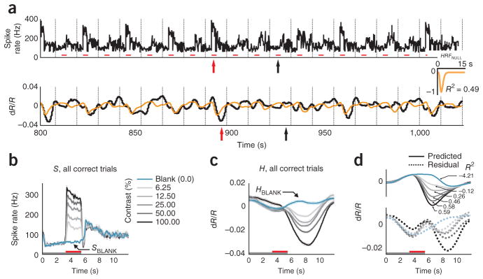
The full hemodynamic signal is poorly predicted by local multi-unit spiking. (a) Top, a section of the full recorded spiking signal (S) for a representative experimental session (black trace). Bottom, corresponding measured hemodynamic signal (H, black) and the best prediction obtained from spiking (orange, $H_{\text{NULL}}^{\text{PRED}}={\mathit{HRF}}_{\text{NULL}}\otimes S$, ⊗ indicates convolution; Supplementary Note, equation (3)). Inset, best fitting kernel HRF_NULL (amplitude normalized) obtained by fitting H to S. Mean R² = 0.49, as calculated using mean signals averaged across contrasts (n = 261 trials total, roughly 43 per contrast). Red line segments indicate stimulus application and vertical dotted lines indicate fixation trial onset. Red and black arrows below traces indicate typical responses to high-contrast (100% contrast) and blank (0% contrast) stimuli, respectively; for hemodynamics, increasing negative amplitudes, that is, increasing absorption of light by cortex, equals increasing blood volume. Note the poor match between the observed and predicted traces leading to a large residual and, consequently, low mean R². (b) Trial-aligned averages of spiking (S) for each contrast. The trial structure is indicated by the color bars (gray, fixate; red, stimulus; no bar, relax). Note the prominent blank-trial spiking signal S_BLANK. (c) Data presented as in b for hemodynamics (H). (d) Data are presented as in b for corresponding predicted hemodynamics $H_{\text{NULL}}^{\text{PRED}}$ (solid lines, top) and residuals ( $H-H_{\text{NULL}}^{\text{PRED}}$, dotted lines, bottom; separated vertically for visibility). Individual R², calculated separately per contrast, are shown alongside each prediction. Data were obtained from monkey S. Error bars represent s.e.m.

To set a null model baseline for alert, task-engaged monkeys, we first determined how well the full recorded local spiking could predict the full recorded hemodynamics. We linearly fitted the measured hemodynamics H to spiking S to generate an optimal linear kernel, HRF_NULL, and the corresponding predicted hemodynamic trace (Fig. 1a and Supplementary Note, equation (1)). Although the prediction appeared to be qualitatively reasonable, quantitatively the match with measured hemodynamics was mediocre, with mean R² = 0.49 (the value calculated for the mean signal averaged over all contrasts; R² is defined as 1 − (variance of residual error)/(variance of measured signal); Supplementary Note, equation (10)).

The inadequacy of the fit was even clearer when we compared predictions with measured signals, contrast by contrast. We obtained poor R² and large residuals that varied with stimulus contrast (Fig. 1d). Notably, R² was poorest for blank trials (0% contrast, R² = −4.21, a negative number as the residual was larger than the measured signal) and improved systematically for stimuli of higher contrast. This suggests that, at low spike rates, the hemodynamic signals may be dominated by non–spike-related components, independent of visual input, such as the previously demonstrated trial-related signals²². Note that the blank-trial spiking signal that adds uniformly to all the spiking responses (S_BLANK; Fig. 1b) is unlikely to be the cause of this mismatch. Being presumably visual, the blank-trial spiking should have linearly predictable hemodynamic correlates, similar to the hemodynamic correlates of the controlled stimuli.

Modified linear model with two signal components

Given the poor fit of the homogeneously linear null model to signals recorded during a task, and the pattern of residual errors by contrast, we considered a simple alternative modified linear model (MLM; Supplementary Fig. 2) for such a task context. This model incorporates our earlier finding of a spike- and stimulus-independent anticipatory trial-related hemodynamic signal²², a signal that is only present in correct trials³². To keep the model as simple as possible, we assumed that the trial-related signal adds linearly^18,20,33 to the visually evoked component; this visually evoked hemodynamic component, we still assumed to be uniformly linearly predicted by visually evoked spiking^1–3, whether driven by controlled stimulation or uncontrolled visual input (as in the blank-trial spiking). We further assumed that the trial-related signal is stereotyped, determined by trial timing alone and is uniformly present in all trials types independent of whether the trial has a visual stimulus or a blank or involves dark-room fixation (Supplementary Note, equation (2)).

This posited structure of the MLM led to two important predictions. First, it predicted that, during visually stimulated tasks, the trial-related hemodynamic signal could be linearly separated from visually evoked responses by subtracting the blank-trial hemodynamic response (H_BLANK: Supplementary Fig. 2 and Supplementary Note, equations (4–6)). Note that this step also uniformly subtracts the hemodynamic correlate of any uncontrolled blank-trial spiking (that is, S_BLANK), thereby revealing responses to the controlled visual stimulus alone. We defined this blank-subtracted signal as the stimulus-evoked hemodynamics, H_STIM; it should be linearly related to the stimulus-evoked spiking, S_STIM, obtained by subtracting blank-trial spiking from the other spike traces. The HRF kernel for the linear part of the MLM could then be estimated by fitting these stimulus-evoked signals against each other (Supplementary Note, equation (7)). Second, it predicted that the trial-related hemodynamic signal seen in visually stimulated tasks should match that seen in dark-room fixation tasks of the same trial timing (Supplementary Note, equations (2, 4–9)). As a corollary, it predicted that the trial-related signal will change to match changes in trial structure, even if the stimulation remained constant.

The MLM led to a marked improvement over the null model. This can be illustrated using the data set described above (Fig. 1), where blank subtraction led to crisp orderly sequences of S_STIM (Fig. 2a) and H_STIM (Fig. 2b). The optimal kernel HRF_STIM (Fig. 2c and Supplementary Note, equations (7,8)) obtained by fitting these stimulus-evoked signals to each other gave a mean R² of 0.99 (versus R² = 0.49 for the null model; Fig 1a, d). The same kernel also made reliable predictions for each individual contrast, closely matching corresponding measured signals H_STIM, with high R², and weak and contrast-independent residuals (Fig. 2c). To assess the statistical significance of these comparisons, we estimated confidence intervals for each value of R² with a bootstrap technique using random selections of the given day’s trials with replacement (200 runs per experiment, see Online Methods). The estimated 95% confidence limits obtained for all R² calculated using the MLM, mean as well as separately by contrast, were comfortably non-overlapping with those of corresponding R² from the null model, emphasizing the high significance of the improvement of the MLM over the null model (Supplementary Fig. 3).

Figure 2.

Results using the MLM: stimulus-evoked (blank subtracted) hemodynamic responses (H_STIM) are reliably and linearly predicted by stimulus-evoked local spiking (S_STIM). (a, b) S_STIM (a) and H_STIM (b) (shaded regions indicate integration windows for calculating mean response strength; see Fig. 3). Data are presented as in Figure 1 with error bars indicating s.e.m. The trial structure is indicated by the color bars (gray, fixate; red, stimulus; no bar, relax). (c) Predicted stimulus-evoked hemodynamics ( $H_{\text{STIM}}^{\text{PRED}}={\mathit{HRF}}_{\text{STIM}}\otimes S_{\text{STIM}}$; Supplementary Note, equation (8)) and corresponding R², contrast by contrast. Dotted traces indicate residuals ( $H_{\text{STIM}}-H_{\text{STIM}}^{\text{PRED}}$). Inset, optimal HRF_STIM (mean R² = 0.99, n = 261 trials). (d) Comparing mean R² for the null model, that is, without blank subtraction (y axis) against the MLM (x axis). Population average (s.e.m.) of mean R² = 0.93 (0.01) for MLM, 0.57 (0.05) for the null model (n = 34 sessions, 3 monkeys). (e) Data are presented as in d for R² calculated separately by contrast and then averaged (one data point per experiment). Fits for the null model were almost all worse than for the MLM (that is, below the diagonal) and included many negative values (shown below scatter plot; population average R² (s.e.m.): MLM, 0.77 (0.03); null model, 0.14 (0.10); n = 34). See Supplementary Figure 3 for bootstrap estimates of confidence intervals. (f) All HRF_STIM kernels (amplitude normalized; color coded by animal; population average latency (s.e.m), 3.1 (0.2) s; population average width (s.e.m.), 3.3 (0.2) s:, n = 34). Inset, average mean R² (s.e.m.) from cross-validation tests using leave-one-out mean kernels, over all animals (0.80 (0.03), n = 34) and separately by animal (monkey S, 0.89 (0.02), n = 17; monkey T, 0.85 (0.03), n = 15; monkey Y, 0.90 (0.01), n = 2). R² pop indicates experimental population average (data from d).

Comparable improvements using the MLM were seen over the population. The MLM gave values of mean R² clustered close to 1.0, much higher than the corresponding values obtained with the null model in essentially every experiment (Fig. 2d). The R² values calculated separately by contrast showed more scatter than the mean R², but even here the null model gave values that were distinctly poorer than those obtained with the MLM, including a number of negative values (Fig. 2e). Again, confidence limits estimated using bootstrapping were used to quantify the significance of these improvements using the MLM (Supplementary Fig. 3d, e).

The individual optimal HRF_STIM kernels were also highly consistent across experiments. All kernels had similar peak latencies and widths (Fig. 2f). In a cross-validation test (see Online Methods), the signal in any experiment was well predicted by the leave-one-out mean kernel averaged over all other experiments, with only a slight improvement in the prediction when conducted separately by animal (Fig. 2f). This consistency of the HRF kernel across experiments and animals suggests that it represents a neurovascular coupling mechanism that is intrinsic to this cortical tissue.

The relationship between stimulus-specific hemodynamics and spiking was robustly linear even though the two signals were individually nonlinear functions of stimulus contrast. This can be seen by comparing the areas under the response curves (Fig. 2a, b). Both the spiking (Fig. 3a) and hemodynamic responses (Fig. 3b) had similar hyperbolic³⁴ relationships to contrast while being homogeneously linear when plotted against each other (Fig. 3c). Note that, unlike in earlier reports¹⁴, the linear regression line (Fig. 3c) passes through the origin with essentially no y intercept or threshold of hemodynamic signal at low spike rate.

Figure 3.

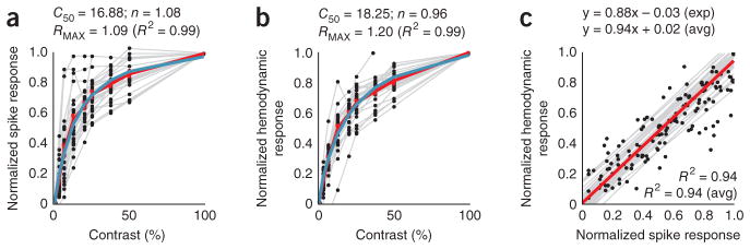
Stimulus-evoked spiking and hemodynamics are hyperbolic functions of stimulus contrast and are linearly related to each other. (a) Normalized stimulus-evoked spike responses across contrasts. Each point shows data for a single contrast on a given session, averaged over the integration window as shown in Figure 2a. Gray lines link sets of points in individual sessions. The red line (piecewise continuous) indicates the average across sessions. The blue line represents the optimal fitted hyperbolic response function R(C) of contrast C, of the form³⁴ $R(C)=R_{max}\left(\frac{C^n}{C^n+C_{50}^n}\right)$; fitted parameters are shown above. (b) Data are presented as in a for stimulus-evoked hemodynamic responses, averaged over the window as in Figure 2b. (c) The spiking and hemodynamic responses shown in a and b, plotted against each other. The gray lines are regression lines for each session and the red line is the average of the regression lines. Expressions show regression and R², both for the experiments in Figures 1 and 2a–c (exp) and the population (avg). Population averages were calculated from session values, weighted by number of trials within a session (n = 34 sessions, 3 monkeys).

Trial-related signal consistent in stimulus and dark room

With the stimulus-evoked portion of the signal well characterized by our MLM model, we next estimated the posited spike- and stimulus-independent trial-related signal T (Fig. 4 and Supplementary Note, equation (2,9)). According to the MLM, this is the signal that remains after subtracting away, from the full measured hemodynamics H, all components that can be predicted from spikes. To estimate spike-predicted components, we used our simplifying assumption that the HRF_STIM kernel can be applied uniformly to all spiking, whether stimulus evoked or uncontrolled (blank trial). The HRF_STIM was obtained, as before (Supplementary Note, equation (7)), by fitting stimulus-evoked spiking (S_STIM; Fig. 4a) to hemodynamics (H_STIM; Fig. 4b). The hemodynamics predicted from full spiking S using this kernel (Fig. 4c) were clearly different from the full measured hemodynamics (Fig. 4b). Qualitatively, however, the latter appear to be a sum of the prediction riding on top of a large contrast-independent response. Indeed, subtracting the predicted from the measured hemodynamics left large remaining signals T that matched each other closely across contrasts. Note, moreover, their substantial strength, which was 1.5-fold greater than that of the maximal H_STIM (compare Fig. 4b with Fig. 4d). It is important to emphasize that, in our framework, these unpredicted hemodynamic signals are not the results of nonspecific spiking (for example, S_BLANK); they comprise the components that, according to the MLM, remain after using HRF_STIM to account for the entirety of the spiking-related hemodynamics, both stimulus evoked and nonspecific (Supplementary Note, equation (9)).

Figure 4.

Estimated trial-related signal T is consistent across contrasts, across experiments, and between stimulated and dark-room trials. (a, b) Spiking (a) and hemodynamics (b) from another representative session. Insets, corresponding S_STIM and H_STIM. The trial structure is indicated by the color bars (gray, fixate; red, stimulus; no bar, relax). (c) Prediction convolving optimal kernel HRF_STIM (inset) with full spiking S (that is, HRF_STIM ⊗S). (d) Estimated trial-related signals (T =〈H −HRF_STIM ⊗ S〉; Supplementary Note, equation (9)) shown individually by contrast; red indicates mean across contrasts. Note the high amplitude of mean T (s.d. = 0.0088, compared with 0.0058 for H_STIM using 100% contrast; a 1.5-fold difference). Note the marked similarity of signals T across contrasts (correlation (Pearson’s r) with leave-one-out means: 0.99, 0.99, 0.99, 0.99, 0.99, 0.99 and 0.96 for contrasts 0–100% in sequence; n = 175 trials, 25 per contrast, 7 contrasts, median r = 0.99). Inset, population histogram of median r (mean (s.e.m.) = 0.94 (0.01), n = 34). (e) Dark-room trials for the sessions shown in a–d. Top, hemodynamic traces, H_DARK. Gray lines are individual traces, all correct trials (n = 45), the green line is the mean of correct trials, and the red line is the prediction, convolving HRF_STIM with dark-room spiking S_DARK (bottom trace, black). Trial structure indicated on time axis (periodic fixations in darkness). (f) Mean trial-related signals T from stimulus-driven (black) and dark-room trials (green), same session (Pearson’s r = 0.94). (g) Signals T as in f for full population (n = 19 pairs, monkey T). (h) Pairwise correlations between stimulated and corresponding dark-room T over population (mean (s.e.m.), pairwise Pearson’s r = 0.61 (0.08), n = 19 pairs).

We quantified the similarity of the trial-related signals T to each other, at different contrasts in an experiment, by correlating the signal T at each contrast (including contrast = 0, blank) with the leave-one-out mean of the signals T calculated at all the other contrasts. All of the resultant correlation (Pearson’s r) values were very close to 1.0 (Fig. 4d). This pattern was repeated over our population of 34 experiments giving, in each case, a median r close to 1.0 (Fig. 4d).

We wanted to test how well the trial-related signals thus calculated matched each other across experiments and how similar they were to the trial-related signals observed in dark-room fixation tasks²². For monkey T, we were successful in getting sets of both dark room and visually stimulated trials in 19 experiments (5 of the current 34, and an additional 14 from a separate project using the same fixation task). Over this population, we found a close match of each residual with the dark-room signal at the same recording site, as well as a marked similarity of these signals across experiments (Fig. 4e–h). As in our earlier published data²², the dark-room trials evoked high-amplitude stereotyped signals of clockwork-like periodicity despite weak spiking (Fig. 4e). However, the dark-room trial-related signal T (that is, after subtracting the, albeit very small, spike-related prediction obtained by convolving with HRF_STIM; Fig. 4e) closely matched the mean trial-related signal T from the visually evoked trials (Fig. 4f). A similar pattern was seen for each experiment. The sets of all dark-room and visually stimulated trial-related signals were markedly similar (Fig. 4g) and matched each other well when correlated pairwise for each recording site (Fig. 4h). This provides compelling evidence for our MLM, that is, that the full hemodynamic signal evoked in an alert task-engaged subject is the linear sum of a spike-related component and a distinct trial-related component that is independent of local spiking or visual stimulation (Supplementary Note, equation (2)).

As an additional test of our premise that the trial-related signal is determined by trial structure independent of stimulus or evoked spiking, we designed a set of experiments in which we varied trial structure while keeping the stimulation parameters unchanged (n = 10 experiments in 2 animals, monkeys S and T; Fig. 5). Both series consisted of 30-s trials with identical stimulation (gratings, with contrasts: 0% (blank), 12.5% or 100% in block-randomized order, shown once per trial). The trials had different fine structure, however. For one set, the monkey made two fixations at 15-s intervals in each 30-s trial (Fig. 5a–c), whereas in the other set, the monkey made three fixations at 10-s intervals per 30-s trial (Fig. 5d–f). The stimulus was presented only during the first fixation, whereas subsequent fixations were on to the blank monitor. Notably, we only considered those trials in which the animal performed sequences of correct fixations extending over the full 30-s trial to be correct trials. Blank trials, correspondingly, consisted of two (Fig. 5a–c) or three (Fig. 5d–f) successive correct blank-monitor fixations starting with the blank (0% contrast) stimulus.

Figure 5.

Estimated trial-related signal T reflects trial timing independent of stimulus timing or contrast. (a, b) Spiking (a) and hemodynamics (b) for trials consisting of fixation sequences in which the animal fixated with 15-s periodicity, but the stimulus (three contrasts, including 0%, blank) was shown at 30-s intervals, that is, only at the first fixation of each pair. Insets, corresponding S_STIM and H_STIM, calculated by subtracting away blank-trial signals consisting of responses to the pair of fixations on to the blank monitor starting with the blank stimulus (indicated by blue curves). Note monophasic stimulus-evoked H_STIM with no evidence of oscillatory rebounds during the blank epoch. The trial structure is indicated by the color bars (gray, fixate; red, stimulus; no bar, relax). (c) T per contrast. Inset, optimal HRF_STIM calculated over 30-s trials. Note that the signal T is close to exactly periodic at the 15-s fixation periodicity, with identical amplitudes for the first and second fixation periods independent of stimulus strength or evoked spikes in the first fixation (correlation of calculated T across stimulus contrasts: 0.98 (median of pairwise correlations between each T and the leave-one-out mean of the other two), n = 74 trials total, roughly 25 per contrast). (d–f) Data are presented as in a–c, with the same stimuli, presented at the same 30-s intervals, but with the monkey fixating every 10 s. The stimulus was shown only on the first fixation of each triplet (n = 83 trials total, roughly 28 per contrast). All error bars indicate s.e.m.

Even though the recorded spiking S, for both trial structures, was dominated by stimulation at the 30-s trial periodicity (Fig. 5a, d), the recorded hemodynamics H showed additional powerful modulations, even for the blank trials (Fig. 5b, e). Notably, this modulation matched the fixation schedule and was thus distinct for the two-fixation versus the three-fixation trials. The signal amplitudes in the second and third intervals were not proportional to the amplitude of the signal in the first fixation interval, as they would have been if they were a result of ringing following the initial stimulation. On subtracting away the relevant blank-trial signals, the stimulus-evoked hemodynamics H_STIM in each case showed a monophasic decline to baseline, with comparable time courses (Fig. 5b, e), as would be expected for a monophasic blood-volume response to the stimulus²⁷. Finally, the trial-related signals T were, in each case, periodic at the trial fine structure with no apparent modulation by the stimulus (T obtained as above by subtracting away from each measured signal H components predicted from full spiking using the relevant HRF_STIM; Fig. 5c, f).

Spikes poorly predict blank-trial and dark-room signals

As a counterproposal to our MLM, it could be argued that there is no need to invoke any special spike-independent trial-related signal T. Although we have provided evidence that blank subtraction leads to a markedly improved linear fit between the stimulus-evoked portions of the signal, it does not follow that the blank-trial hemodynamics necessarily contain signal components independent of spiking as proposed in the MLM. Instead, it could be that blank-trial hemodynamics are related linearly to the sometimes substantial blank-trial spiking (Fig. 1b) through a distinct HRF kernel appropriate for low spiking levels that is very different from the kernel linking the stimulus-evoked signals. This, one could argue, is the reason for the mismatch when trying to predict the full hemodynamics from the full spiking (Fig. 1). As we show below, however, any such distinct HRF kernels appear arbitrarily variable and unreliable, making this counterproposal highly nonparsimonious and thus implausible.

We first tested whether the blank-trial hemodynamics could be predicted linearly from spiking alone (Fig. 6a–d and Supplementary Note, equation (11)), as opposed to being modeled by a sum of spike-predicted and trial-related components (that is, MLM; Supplementary Note, equation (4)). Indeed, we could make a reasonable prediction (R² = 0.46; Fig. 6a) by using the optimal blank-fitted kernel HRF_BLANK obtained by fitting the blank-trial hemodynamics to blank-trial spiking. This was better than the value of R² = −0.19 for the prediction using the same session’s HRF_STIM (Fig. 6a). This, however, is not surprising. By definition, the fitting process discovers a kernel that maximally accounts for the variance in the fitted signal. However, the fit here was likely fortuitous. The blank-fitted kernel was fivefold larger in amplitude and opposite in sign to the HRF_STIM, giving absurd predictions for the stimulus-evoked signal when convolved with the same session’s stimulus-evoked spiking S_STIM (Fig. 6b). Over the population, these blank-fitted kernels were highly variable in amplitude relative to the corresponding HRF_STIM (Fig. 6c) and, moreover, showed a wide scatter in peak latency and width (Fig. 6c, d). Notably, the presence of both positive and negative amplitudes made it meaningless to even perform a cross-validation test to see how well the kernel from one day can be used to predict the blank signals from other days, in sharp contrast to the reliable predictions obtained through cross-validation for the HRF_STIM (Fig. 2f).

Figure 6.

Blank-trial and dark-room hemodynamic responses are poorly fitted to spiking. (a) Blank-trial responses (same experiment as shown in Fig. 4). Top, S_BLANK. Bottom, corresponding H_BLANK comparing the measured value (blue) with two alternative predictions: one from S_BLANK using session’s stimulus-fitted kernel (red, HRF_STIM ⊗S_BLANK, R²= −0.19, n = 25 trials) and the other using the optimal blank-fitted kernel (brown, HRF_BLANK ⊗S_BLANK, R² = 0.46). Inset, the blank-fitted kernel HRF_BLANK (amplitude normalized to HRF_STIM). Gray bar indicates fixation. (b) Predictions (HRF_BLANK ⊗S_STIM) of stimulus-evoked hemodynamics using blank-fitted kernel. Compare with measured H_STIM (inset) (mean R² = −11.9). (c) Population of HRF_BLANK kernels, each normalized by amplitude of corresponding HRF_STIM kernel. Inset, histogram of HRF_BLANK amplitudes normalized by corresponding HRF_STIM (Amp. Blank/Stim., n = 34). (d) Peak latencies (left) and widths (right) of HRF_BLANK versus HRF_STIM. Note the high variability (s.e.m.) in both parameters for the HRF_BLANK. Population average latency (s.e.m): blank, 4.6 (0.6) s; stimulus, 3.1 (0.2) s; population average width (s.e.m.): blank, 5.8 (1.0) s; stimulus, 3.3 (0.2) s; n = 33; ignoring one outlier with width = 1.25 × 10⁸ s for the blank). (e) Data are presented as in a for the dark-room task (data from Fig. 4e). Top, S_DARK. Bottom, corresponding H_DARK comparing measured trace (green) with prediction using the optimal dark-fitted kernel (magenta, HRF_DARK ⊗S_DARK, R² = 0.58). Inset, dark-fitted kernel HRF_DARK (amplitude normalized to HRF_STIM). (f) Top, HRF_BLANK kernels normalized by absolute values of their own amplitudes (note variability in time courses). Bottom, HRF_DARK kernels normalized by corresponding HRF_BLANK amplitudes. Inset, histogram of HRF_DARK amplitudes normalized by HRF_BLANK (Amp. Dark/Stim., n = 19 sessions). (g) Scatter plots of peak latencies (top, Pearson’s r = 0.04) and widths (bottom, r =0.07) comparing HRF_DARK and corresponding HRF_BLANK (n = 18; outlier ignored as in d).

The presence of both dark-room and visually stimulated trials for 19 recording sites allowed for additional tests of the counterproposal to the MLM. If there exist valid low-spiking-level kernels linearly linking blank-trial spiking to hemodynamics, then such kernels should also be reasonable for linking dark-room spiking to hemodynamics. We tested this possibility by calculating the optimal dark-fitted kernels for each of these sessions (Supplementary Note, equation (12)). These kernels, again provided, by definition, good fits for the given dark-room signals; but they were arbitrarily different from the corresponding blank-fitted kernels. Thus, for the particular example session, the dark-fitted kernel was opposite in sign and much larger in amplitude (40-fold versus fivefold larger than the amplitude of the session’s HRF_STIM; Fig. 6e), reflecting the smaller dark-room spiking amplitude compared with blank-trial spiking. Over the population, we found similarly poor correspondence in amplitude, latency and width between dark- and blank-fitted kernels (Fig. 6f, g). The apparently arbitrary shapes and sizes of these kernels, when combined with our earlier evidence for lawful and stereotyped trial-related signals when fitting the MLM (Figs. 4 and 5), strongly suggest that dark- and blank-fitted kernels reflect only accidental matches linking weak residual spikes to hemodynamics that are actually dominated by spike- independent trial-related signals.

Blank subtraction required to estimate spikes from imaging

The primary use of neuroimaging is as a proxy for local neural activity. We wanted to quantify the importance of blank subtraction when equating the imaging signal with neural response. To this end, we compared the validity with which we could deduce measured spiking from full versus blank-subtracted hemodynamics by deconvolving²⁸ with the relevant optimal HRF. We expected that deconvolving a given blank-subtracted (that is, stimulus evoked) signal H_STIM using its optimal kernel HRF_STIM would trivially return a valid estimate of the corresponding blank-subtracted (that is, stimulus evoked) spiking S_STIM, as these signals were well fitted to each other. What we wanted to assess, for comparison, was the reliability with which the full measured spiking S could be obtained from the full hemodynamics H using a similar deconvolution with its optimal kernel HRF_NULL. Given that convolution is equivalent to the product of Fourier transforms in frequency space, we deconvolved by dividing the Fourier transform of the hemodynamic signal by the Fourier transform of the relevant HRF kernel. As HRFs have very little power at high temporal frequencies, reflecting the slow time course of the hemodynamic response²⁷, we restricted the effective frequency range of this division with an appropriate filter in frequency space to prevent amplifying high-frequency noise in the hemodynamic signal (Online Methods).

As expected, the estimate of spiking obtained by deconvolving the mean H_STIM with HRF_STIM closely matched the measured S_STIM, albeit without the high-frequency features (mean R² = 0.64 for the predicted spike trace; Fig. 7a, b). The match was even better when comparing the estimated spiking not with S_STIM, but with its low pass–filtered version, using the same filter as used for the deconvolution (mean R² = 0.82; Fig. 7b and Online Methods).

Figure 7.

Blank-subtracted, but not full, hemodynamic signal is a good proxy for local spiking responses. (a) Mean stimulus-evoked (that is, blank subtracted) hemodynamic response H_STIM averaged across contrasts for one experimental session. Inset, corresponding HRF_STIM (n = 162 trials, roughly 41 per contrast, mean R² = 0.93). The trial structure is indicated by the color bars (gray, fixate; red, stimulus; no bar, relax). (b) Mean stimulus-evoked spiking. Thin black line, mean stimulus-evoked (blank subtracted) measured spiking S_STIM. Thick black line, low pass–filtered mean stimulus-evoked spiking S_STIM. Red, spiking estimated by deconvolving H_STIM with HRF_STIM. Note the good match with measured S_STIM (R² = 0.82 with low pass–filtered S_STIM, R² = 0.64 without low-pass filtering). (c) Mean full hemodynamics H: same data as in a, but without blank subtraction. Inset, corresponding HRF_NULL. Note the poor mean R² = 0.37 compared with HRF_STIM. (d) Mean full spiking without blank subtraction. Thin black line, mean measured spiking S. Thick black line, low pass–filtered mean measured spiking S. Orange, spiking estimated by deconvolving H with HRF_NULL (R² = −0.53). Red, spiking estimated by deconvolving H with HRF_STIM (R² = −1.18; session mean spike rate added to deconvolved signals to align with measured spikes on vertical axis). Note the poor match of either estimate with measured full (low pass–filtered) spiking S. (e) Comparing R² for estimates of spiking from full and stimulus-evoked hemodynamic signals over the population. Orange, H_STIM deconvolved with HRF_STIM and H deconvolved with HRF_NULL. Red, both H_STIM and H deconvolved using HRF_STIM. Note the uniformly high R² for estimating S_STIM from H_STIM (mean R² (s.e.m.) = 0.85 (0.02), n = 34) versus low R², including many large negative values for estimating S from full H (using HRF_STIM, mean R² = −2.5 (0.9); using HRF_NULL, mean R² = −2.5 (1.0); n = 34).

In contrast, deconvolving the full H using HRF_NULL (Fig. 7c) gave an estimate of neural spiking that poorly matched the mean full S, with large oscillations following the primary peak (mean R² = −0.53; Fig. 7d). As a control, we tried deconvolving not with HRF_NULL, but with HRF_STIM, as the latter is arguably a better optimal kernel for this data set. This estimate of neural activity was no better (mean R² = −1.18; Fig. 7d). Comparable results were seen over the population (Fig. 7e), where the measured stimulus-evoked (that is, blank subtracted) spiking was uniformly well estimated from stimulus-evoked hemodynamics. In contrast, the full spiking was very poorly estimated from the corresponding full hemodynamics, whether the deconvolution was performed using HRF_STIM or HRF_NULL.

DISCUSSION

We used simultaneous optical imaging and electrode recording to relate cortical neuroimaging signals to local neural spiking in alert subjects performing periodic sensory tasks (from V1 of macaque monkeys performing periodic visual tasks). We demonstrate a parsimonious model of the measured imaging signal, the MLM. In our model, the measured imaging signal is a linear sum of two distinct components: a spike-associated component tightly related to stimulus intensity and local spiking, and a trial-related component that seems to be determined only by the timing and structure of the task, independent of stimulus or local spiking. The trial-related component can be removed linearly, for example, by subtracting the responses to blank trials (Fig. 2) that have exactly the same timing structure as stimulated trials (Fig. 5b, e). This blank subtraction leaves a stimulus- evoked signal (Supplementary Note, equation (6)) that is homogenously linear with stimulus-evoked local spiking over the full range of stimulus intensity from baseline to near-maximal (Figs. 2a–c and 3, and Supplementary Note, equation (7)). The HRF kernel relating these two signals is largely invariant in shape across recording sites and animals (five hemispheres, three monkeys; Fig. 2f), suggesting that it reflects the true neurovascular coupling in this cortical region. By the same token, this stimulus-evoked neuroimaging signal is a faithful proxy for the stimulus-evoked local spiking (Fig. 7). In contrast with the excellent fit of the stimulus-evoked signals, the second component of our model, the trial-related signal, has a notably poor fit to local spiking (Fig. 6). It is, however, reliably trial-locked and robust across stimulus conditions, including total darkness (Figs. 4d–h and 5c, f). Given that the amplitude of the trial-related signal can exceed the maximal stimulus-evoked signal (Fig. 4), failure to account for it properly can lead to marked errors when using the neuroimaging signal to estimate neural spiking (Fig. 7).

It is instructive to compare our results with the body of recent work relating neural spiking to hemodynamics^2,3,14. First, our results suggest that a simple linear model, with the critical addition of the trial-related, spike-independent signal component, can, in fact, reveal a reliable quantitative relationship between the spike rate of neurons and the hemodynamic response, in contrast with earlier results that have suggested the lack of any such relationship¹⁴. Note, however, that the good prediction of stimulus-specific hemodynamics from spiking does not imply that spiking causes hemodynamics³⁵; the actual signals driving hemodynamics are as yet poorly understood³⁶. Next, our observed homogenous linear relationship between stimulus-evoked spiking and hemodynamics (Fig. 3) differs from the pronounced threshold nonlinearity reported earlier¹⁴. This difference is unlikely to be a result of trial-related signals, as the previous study was conducted using anesthetized animals. It could be an artifact of anesthesia or it may be a nonlinearity in neurovascular coupling resulting from the long stimulus durations used, up to 24 s, versus the shorter and more natural 2–3 s that we used. Understanding this difference should provide valuable insights into neurovascular coupling.

Although our use of the cortical blood volume signal may have made it easier to validate our model, our findings should be broadly applicable to all hemodynamics-based neuroimaging techniques, including blood oxygen level–dependent (BOLD) fMRI. The monophasic blood-volume impulse response to stimulus-evoked spikes^27,29–31 allowed us to fit the stimulus-evoked signals with high reliability using a single gamma-variate kernel and minimal free parameters. By the same token, it allowed us to unambiguously deconvolve hemodynamics and estimate spiking. This let us easily demonstrate key features of the MLM, including the linear separation of stimulus- and task-related signal components. The more complex BOLD and other blood oxygenation–related signals with their multiphasic responses and ringing^37,38 could have made fitting hemodynamics to spiking technically more challenging and possibly more ambiguous. However, given our results using the blood volume signal, we expect to see effects in BOLD fMRI that are qualitatively very similar. Although the quantitative relationship between BOLD and blood volume varies across brain regions and even across cortical layers³⁹, the two signals mostly track each other closely in overall time course in an individual brain region³⁹. The strengths of both signals are similarly graded in response to stimulus strength, including similarly non-monotonic and sign-reversed responses⁴⁰. Both BOLD fMRI and blood volume signals also share overall broad time courses with concurrent intrinsic- signal optical imaging and can be reliably predicted from the latter²⁶. Finally, it should be noted that at least two groups measuring BOLD fMRI signals in humans have, as we have, reported stimulus- independent task-related signals entrained to task timing that need to be subtracted linearly from the overall neuroimaging signal to relate hemodynamics to sensory stimulation^9,18,20 (these studies, being in humans, did not include electrodes in the brain to examine the neural underpinnings of the task-related signals).

Our findings have a substantial bearing on the growing field of functional neuroimaging in alert task-engaged subjects. It is now clear that such imaging signals contain robust non-sensory components reflecting, for example, anticipatory attention, task structure and response preparation^{18–20,41–44}. Our trial-related signal likely belongs to the same class. At a practical level, our combination of imaging and electrode recordings quantifies both the effectiveness and critical necessity of task designs that subtract away this task-related non-sensory signal. A number of currently used task designs, proposed earlier on empirical grounds, already do so effectively; these include designs that linearly subtract either blank^9,24,45 or nonspecific global from local signals^20,33, designs that contrast one sensory stimulus against another in a common task structure^46,47, and designs that regress the hemodynamic signal against a range of stimulus intensities^10,12. Notably, for such subtraction to properly reveal stimulus-related signals, the subtracted trial presumably needs to be identical to stimulated trials in all respects (timing, reward, evoked anticipation, etc.), differing only in not containing the stimulus of interest.

At another level, however, the robust link between stimulus-evoked hemodynamics and spiking throws into sharper relief the lack of such a link for the trial-related signal and suggests that other non-sensory signals may be similarly poorly related to local spiking^18,20. For example, there is a well-known discrepancy between robust fMRI evidence for attentional modulation in human V1 (ref. 42) and the lack of such modulation in electrode recordings from macaques⁴⁸. Our findings raise the possibility that this entire class of non-sensory signals could have neural underpinnings distinct from sensory-driven spiking activity. The trial-related signal described here is also distinct from the coherent ongoing V1 activity imaged in anesthetized animals⁴⁹, as the latter was closely correlated with local spiking and LFP⁴⁹. The trial-related signal may involve neuromodulatory³⁶ input from some brain stem center that tracks behavioral timing or it may reflect feedback from some higher cortical center. Furthermore, it could act preferentially on cells other than pyramidal neurons, such as interneurons or astrocytes. There is also the possibility of direct neuromodulatory control of blood vessels giving rise to the hemodynamic signal⁵⁰. Finally, when interpreting recorded hemodynamics as a measure of local neural activity, it remains to be established whether the strength of the trial-related signal can be equated with that of stimulus-evoked signals on any common measure, such as a metabolic one of energy consumption.

A number of additional questions remain. We have demonstrated the MLM for area V1. It would be important to see how well it generalizes over other brain regions. Furthermore, we controlled spike rate by varying the contrast of large, uniform gratings, which changes activity monotonically over the population of activated neurons. We could get valuable insights by controlling spike rates in a manner that differentially targets different neuronal populations, for example, by having punctate stimuli, thereby possibly getting different rates of spatial drop-off in different signals (LFP, spiking, hemodynamics). We noted that the goodness of fit between sensory hemodynamics and gamma-band LFP was much more variable than with spiking (data not shown), in contrast with earlier reports¹⁴. Finding answers to these questions would be critical for interpreting functional brain imaging.

ONLINE METHODS

Summary

Simultaneous intrinsic-signal optical imaging and electrophysiology were acquired from alert macaques engaged in passive fixation tasks (n = 34 sites, 5 hemispheres in 3 monkeys, plus 14 additional experiments) using methods developed previously^22–24. All experimental procedures were performed in accordance with the US National Institutes of Health Guide for the Care and Use of Laboratory Animals and were approved by the Institutional Animal Care and Use Committees of Columbia University and the New York State Psychiatric Institute.

Behavior and stimuli

Animals held fixation periodically for juice reward, cued by the color of a fixation spot (fixation window, 1.0–3.5 degrees in diameter; monitor distance, 133 cm; fixation duration, 3–4 s; trial duration, 10–20 s). For experiments with visual stimulation, stimuli consisted of sine-wave gratings (contrasts, 0% (blank), 6.25%, 12.5%, 25%, 50% and 100%; mean luminance = background luminance = 46 cd m⁻²; spatial frequency, 2 cycles per degree; drift speed, 4 degrees per s; diameter, 2–4 degrees; orientation optimized for the electrode recording site). Trials typically comprised single fixations, with stimulus presented during fixation. For some experiments (Fig. 5), trials comprised sequences of two or three fixations with the stimulus presented only on the first fixation. Stimuli were block randomized, that is, presented in blocks each containing a single full set of contrasts in random order. In the block, stimuli were repeated following errors (incorrect fixation) until the animal had a correct trial for each stimulus in a block (for multi-fixation trials, all fixations had to be correct for a trial to be correct). Some experiments included 3.125% contrast for finer resolution at low contrasts; some others used a reduced set of contrasts to increase the number of trials per condition. Dark-room experiments were performed in a completely dark room with the monitor covered and the fixation point behind a pinhole (as described in ref. 22). Eye fixation and pupil diameter were recorded using an infrared eye tracker⁵¹.

Surgery, recording chambers and artificial dura

After the monkeys were trained on visual fixation tasks, craniotomies were performed over the animals’ V1 and glass-windowed stainless steel recording chambers were implanted, under surgical anesthesia, using standard sterile procedures²⁴, to image a ~10-mm area of V1 covering visual eccentricities from ~1 to 5°. The exposed dura was resected and replaced with a soft, clear silicone artificial dura. After the animals had recovered from surgery, their V1 was optically imaged, routinely, while they engaged in the fixation task. Recording chambers and artificial dura were fabricated in our laboratory using published methods⁵².

Hardware

Camera, Dalsa 1M30P (binned to 256 × 256 pixels, 7.5 or 15 frames per s); frame grabber, Optical PCI Bus Digital (Coreco Imaging). Software was developed in our laboratory based on a previously described system⁵³. Illumination, high-intensity LEDs (Agilent Technologies, Purdy Technologies) with emission wavelength centered at 530 nm (green, equally absorbed in oxy- and deoxyhemoglobin). Lens, macroscope of back-to-back camera lenses focused on the cortical surface. Imaging, trial data (trial onset, stimulus onset, identity and duration, etc.) and behavioral data (eye position, pupil size, timing of fixation breaks, fixation acquisitions, trial outcome) were acquired continuously. Data analyses were performed offline using custom software in MATLAB (MathWorks).

Image pre-processing

Prior to analysis, acquired images were (if necessary) motion corrected by aligning each frame to the first frame by shifting and rotating the images using the blood vessels as a reference⁵⁴. Slow temporal drifts (>30 s) were removed with high-pass filtering, and cortical pulsations with low-pass filtering using the Chronux MATLAB Toolbox function runline.m (typical heart rates were ~2–3 Hz, much faster than the typical hemodynamic response frequencies of ~<0.5 Hz).

Electrophysiology

Electrode recordings were made simultaneously with optical imaging. Recording electrodes (FHC, AlphaOmega; typical impedances were ~600–1,000 kΩ) were advanced into the recording chamber through a silicone-covered hole in the external glass window, using a custom-made low-profile microdrive. Recording sites were mostly, but not exclusively, confined to upper layers. Signals were recorded and amplified using a Plexon recording system. The electrode signal was split into spiking (100 Hz to 8 kHz bandpass) and LFP (0.7–170 Hz); LFP data not shown. No attempt was made at isolating single units and all measured spiking was MUA (defined as each negative-going crossing of a threshold = ~4× the r.m.s. of the baseline obtained while the animal looked at a grey screen²²). The MUA signals were then high-pass filtered to remove slow drifts (>30 s), down sampled to the imaging frame rate (7.5 or 15 samples per s) and aligned offline with the images.

HRF kernel fitting

Each HRF was modeled as a gamma-variate function kernel of the form

$$\mathit{HRF}(t,T,W,A)=A★{\left(\frac{t}{T}\right)}^{\alpha }★exp\left(\frac{t-T}{-\beta }\right)$$

where α=(T/W)² * 8.0 * log(2.0), β=W²/(T * 8.0 * log(2.0)), A is the amplitude, T is the time to peak and W is the full width at half maximum^8,22,55. This functional form allows for parametrically varying kernel amplitude, latency and width. For fitting, we used a downhill simplex algorithm (fminsearch, MATLAB) minimizing the sum square difference between measured and predicted hemodynamics. All fits used periodic functions (30 repetitions) constructed from means of the relevant signals across contrasts, aligned to trial onsets, for correct trials alone. Thus, HRF_STIM was obtained by fitting a periodic pattern of the mean S_STIM to the mean H_STIM, the HRF_NULL by fitting the mean S to the mean H (over correct trials alone), the HRF_BLANK by fitting the mean S_BLANK to the mean H_BLANK, and the HRF_DARK by fitting the mean S_DARK to the mean H_DARK.

Goodness of fit of predicted hemodynamics

Fit was quantified as R² = 1 − (variance of the residual error)/(variance of measured hemodynamics) (Supplementary Note, equation (10)), expressed either separately for each contrast or as mean R², that is, calculated for the mean signals averaged across all contrasts. For all fits other than of the blank signal, predictions (and residual errors) were calculated by convolving the full raw measured spike trace with the relevant HRF and then separating later into correct trials by contrast, or averaging across contrasts. This is more reliable than convolving synthetic periodic functions constructed from mean signals because with periodic functions there is a risk of getting a match, not with the true signal, but with a signal phase-shifted by a fraction of a trial period⁵⁶. Such mismatches are highly unlikely in the measured signal with its random sequence of stimulus intensities and corresponding evoked hemodynamics⁵⁶. The blank signal fit using HRF_BLANK was tested using periodic functions, as in this case we were testing the fit using a kernel that specifically did not fit the full stimulated spike sequence.

Bootstrapping to get confidence limits on R²

For each experiment, 200 bootstrap data sets were constructed, each with the same number of trials as the original, using random resampling with replacement (Supplementary Fig. 3). The resampled hemodynamic and spike trials were then fitted against each other separately for both models (MLM and null) and R² values were calculated as before (Supplementary Note, equation (10)). The 95% confidence limits were obtained by taking the 2.5^th to the 97.5^th percentiles; similarly, 80% confidence limits by taking the 10^th to the 90^th percentile. Random reselection was done separately by contrast to have the same number of trials per contrast. However, each contrast used the same random number set to maintain stimulus blocks and reduce variability resulting from long-term drifts in physiology or recording stability. This was particularly necessary for the MLM, which involves subtracting the mean blank signals 〈H_BLANK〉 and 〈S_BLANK〉 from all other contrasts; if blocks are not maintained, this subtraction leads to a number of noisy outliers in the bootstrap estimate when a set of blanks trials dominated by one epoch of a session (for example, high signal) is subtracted from nonblank trials dominated by a different epoch (for example, low signal).

Cross-validation of HRF_STIM kernels across sessions

For each session, we created a leave-one-out mean HRF_STIM kernel by averaging the two timing parameters (peak latency and width) across all kernels excluding the given one. Kernel amplitude was obtained by fitting, using this mean kernel to fit the given session’s data (HRF_STIM amplitude depends on an arbitrary scale factor in electrode recording; Supplementary Fig. 4). This leave-one-out mean kernel with the best fitted amplitude was then used to obtain the cross-validation prediction and corresponding R². Cross-validation was performed either across all animals or restricting the leave-one-out averaging to other kernels for the given animal.

Deconvolution

The spike trace estimated by deconvolution was defined as $D=F^{-1}\left\{\frac{F(H)}{F(\mathit{HRF})}\right\}$, where H is the relevant hemodynamic signal, HRF is the corresponding optimal HRF kernel and F and F⁻¹ indicate forward and inverse (fast) Fourier transforms, respectively. Given that F(HRF) has low power at high frequencies, reflecting the slow hemodynamic response, we filtered using a Hamming window with a 0.5-Hz cutoff in frequency space. This avoided high-frequency noise in the hemodynamic signal from being amplified during deconvolution. The same filter was used to discount high frequencies in the measured spike rate before correlating with the deconvolved estimate.

Checking the stability of our primary findings against variability in electrode recordings

If measured spiking S is a veridical scaled sample of the true spiking s of our models despite measurement variability across experiments (different electrodes, different thresholds for spike detection for MUA), then the amplitude of the fitted HRF should simply scale inversely with measured spiking for a given experiment (Supplementary Fig. 4 and Supplementary Note, equation (7))

$${\mathit{HRF}}_{\text{STIM}}\otimes S_{\text{STIM}}\approx \mathit{hrf}\otimes s_{\text{STIM}}\approx H_{\text{STIM}}$$ (1)

The scale factor (between the measured S and the true s) will cancel out in all equations for a given experiment, leaving model features unchanged (that is, kernel shape, trial-related signal T and R²). We tested for this in two ways. First, we tested the effect of varying spike detection thresholds. In five experiments, we recorded the electrode signal at a low threshold and then rethresholded off-line to generate multiple sets of spiking data S for the same imaging data (for example, peak spike rates from about 300 s⁻¹ to about 10 s⁻¹ for progressively higher thresholds; Supplementary Fig. 4a, b). These rethresholded spike data were then fitted separately against the common imaging signal (Supplementary Fig. 4c–g). In a second test, we checked the linearity of the relation linking HRF_STIM amplitude against the inverse of the S_STIM amplitude over our full data set (integration window for mean S_STIM coextensive with stimulus duration as in Fig. 2a; Supplementary Fig. 4h).

References

- 1.Boynton GM, Engel SA, Glover GH, Heeger DJ. Linear systems analysis of functional magnetic resonance imaging in human V1. J Neurosci. 1996;16:4207–4221. doi: 10.1523/JNEUROSCI.16-13-04207.1996. [DOI] [PMC free article] [PubMed] [Google Scholar]
- 2.Heeger DJ, Huk AC, Geisler WS, Albrecht DG. Spikes versus BOLD: what does neuroimaging tell us about neuronal activity? Nat Neurosci. 2000;3:631–633. doi: 10.1038/76572. [DOI] [PubMed] [Google Scholar]
- 3.Rees G, Friston KJ, Koch C. A direct quantitative relationship between the functional properties of human and macaque V5. Nat Neurosci. 2000;3:716–723. doi: 10.1038/76673. [DOI] [PubMed] [Google Scholar]
- 4.Heeger DJ, Ress D. What does fMRI tell us about neural activity? Nat Rev Neurosci. 2002;3:142–151. doi: 10.1038/nrn730. [DOI] [PubMed] [Google Scholar]
- 5.Friston KJ, Jezzard P, Turner R. Analysis of functional MRI time-series. Hum Brain Mapp. 1994;1:153–171. [Google Scholar]
- 6.Josephs O, Turner R, Friston KJ. Event-related fMRI. Hum Brain Mapp. 1997;5:243–248. doi: 10.1002/(SICI)1097-0193(1997)5:4<243::AID-HBM7>3.0.CO;2-3. [DOI] [PubMed] [Google Scholar]
- 7.Dale AM, Buckner RL. Selective averaging of rapidly presented individual trials using fMRI. Hum Brain Mapp. 1997;5:329–340. doi: 10.1002/(SICI)1097-0193(1997)5:5<329::AID-HBM1>3.0.CO;2-5. [DOI] [PubMed] [Google Scholar]
- 8.Cohen MS. Parametric analysis of fMRI data using linear systems methods. Neuroimage. 1997;6:93–103. doi: 10.1006/nimg.1997.0278. [DOI] [PubMed] [Google Scholar]
- 9.Pestilli F, Carrasco M, Heeger DJ, Gardner JL. Attentional enhancement via selection and pooling of early sensory responses in human visual cortex. Neuron. 2011;72:832–846. doi: 10.1016/j.neuron.2011.09.025. [DOI] [PMC free article] [PubMed] [Google Scholar]
- 10.Engel S, Zhang X, Wandell BA. Colour tuning in human visual cortex measured with functional magnetic resonance imaging. Nature. 1997;388:68–71. doi: 10.1038/40398. [DOI] [PubMed] [Google Scholar]
- 11.Buckner RL, et al. Functional-anatomic correlates of object priming in humans revealed by rapid presentation event-related fMRI. Neuron. 1998;20:285–296. doi: 10.1016/s0896-6273(00)80456-0. [DOI] [PubMed] [Google Scholar]
- 12.Boynton GM, Demb JB, Glover GH, Heeger DJ. Neuronal basis of contrast discrimination. Vision Res. 1999;39:257–269. doi: 10.1016/s0042-6989(98)00113-8. [DOI] [PubMed] [Google Scholar]
- 13.Grill-Spector K, Malach R. fMR-adaptation: a tool for studying the functional properties of human cortical neurons. Acta Psychol (Amst) 2001;107:293–321. doi: 10.1016/s0001-6918(01)00019-1. [DOI] [PubMed] [Google Scholar]
- 14.Logothetis NK, Pauls J, Augath M, Trinath T, Oeltermann A. Neurophysiological investigation of the basis of the fMRI signal. Nature. 2001;412:150–157. doi: 10.1038/35084005. [DOI] [PubMed] [Google Scholar]
- 15.Mukamel R, et al. Coupling between neuronal firing, field potentials and fMRI in human auditory cortex. Science. 2005;309:951–954. doi: 10.1126/science.1110913. [DOI] [PubMed] [Google Scholar]
- 16.Gardner JL, et al. Contrast adaptation and representation in human early visual cortex. Neuron. 2005;47:607–620. doi: 10.1016/j.neuron.2005.07.016. [DOI] [PMC free article] [PubMed] [Google Scholar]
- 17.Boynton GM. Spikes, BOLD, attention and awareness: a comparison of electrophysiological and fMRI signals in V1. J Vis. 2011;11:12. doi: 10.1167/11.5.12. [DOI] [PMC free article] [PubMed] [Google Scholar]
- 18.Jack AI, Shulman GL, Snyder AZ, McAvoy MP, Corbetta M. Separate modulations of human V1 associated with spatial attention and task structure. Neuron. 2006;51:135–147. doi: 10.1016/j.neuron.2006.06.003. [DOI] [PubMed] [Google Scholar]
- 19.Sylvester CM, Shulman GL, Jack AI, Corbetta M. Asymmetry of anticipatory activity in visual cortex predicts the locus of attention and perception. J Neurosci. 2007;27:14424–14433. doi: 10.1523/JNEUROSCI.3759-07.2007. [DOI] [PMC free article] [PubMed] [Google Scholar]
- 20.Donner TH, Sagi D, Bonneh YS, Heeger DJ. Opposite neural signatures of motion-induced blindness in human dorsal and ventral visual cortex. J Neurosci. 2008;28:10298–10310. doi: 10.1523/JNEUROSCI.2371-08.2008. [DOI] [PMC free article] [PubMed] [Google Scholar]
- 21.Maier A, et al. Divergence of fMRI and neural signals in V1 during perceptual suppression in the awake monkey. Nat Neurosci. 2008;11:1193–1200. doi: 10.1038/nn.2173. [DOI] [PMC free article] [PubMed] [Google Scholar]
- 22.Sirotin YB, Das A. Anticipatory haemodynamic signals in sensory cortex not predicted by local neuronal activity. Nature. 2009;457:475–479. doi: 10.1038/nature07664. [DOI] [PMC free article] [PubMed] [Google Scholar]
- 23.Bonhoeffer T, Grinvald A. Optical imaging based on intrinsic signals: the methodology. In: Toga AW, Mazziotta JC, editors. Brain Mapping: The Methods. Academic Press; San Diego: 1996. [Google Scholar]
- 24.Shtoyerman E, Arieli A, Slovin H, Vanzetta I, Grinvald A. Long-term optical imaging and spectroscopy reveal mechanisms underlying the intrinsic signal and stability of cortical maps in V1 of behaving monkeys. J Neurosci. 2000;20:8111–8121. doi: 10.1523/JNEUROSCI.20-21-08111.2000. [DOI] [PMC free article] [PubMed] [Google Scholar]
- 25.Fukuda M, Moon CH, Wang P, Kim SG. Mapping iso-orientation columns by contrast agent-enhanced functional magnetic resonance imaging: reproducibility, specificity and evaluation by optical imaging of intrinsic signal. J Neurosci. 2006;26:11821–11832. doi: 10.1523/JNEUROSCI.3098-06.2006. [DOI] [PMC free article] [PubMed] [Google Scholar]
- 26.Kennerley AJ, et al. Refinement of optical imaging spectroscopy algorithms using concurrent BOLD and CBV fMRI. Neuroimage. 2009;47:1608–1619. doi: 10.1016/j.neuroimage.2009.05.092. [DOI] [PMC free article] [PubMed] [Google Scholar]
- 27.Sirotin YB, Hillman EMC, Bordier C, Das A. Spatiotemporal precision and hemodynamic mechanism of optical point-spreads in alert primates. Proc Natl Acad Sci USA. 2009;106:18390–18395. doi: 10.1073/pnas.0905509106. [DOI] [PMC free article] [PubMed] [Google Scholar]
- 28.Glover GH. Deconvolution of impulse response in event-related BOLD fMRI. Neuroimage. 1999;9:416–429. doi: 10.1006/nimg.1998.0419. [DOI] [PubMed] [Google Scholar]
- 29.Devor A, et al. Coupling of total hemoglobin concentration, oxygenation and neural activity in rat somatosensory cortex. Neuron. 2003;39:353–359. doi: 10.1016/s0896-6273(03)00403-3. [DOI] [PubMed] [Google Scholar]
- 30.Sheth SA, et al. Linear and nonlinear relationships between neuronal activity, oxygen metabolism and hemodynamic responses. Neuron. 2004;42:347–355. doi: 10.1016/s0896-6273(04)00221-1. [DOI] [PubMed] [Google Scholar]
- 31.Nemoto M, et al. Functional signal- and paradigm-dependent linear relationships between synaptic activity and hemodynamic responses in rat somatosensory cortex. J Neurosci. 2004;24:3850–3861. doi: 10.1523/JNEUROSCI.4870-03.2004. [DOI] [PMC free article] [PubMed] [Google Scholar]
- 32.Sirotin YB, Cardoso MMC, Lima BR, Das A. Spatial homogeneity and task-synchrony of the trial-related hemodynamic signal. Neuroimage. 2012;59:2783–2797. doi: 10.1016/j.neuroimage.2011.10.019. [DOI] [PMC free article] [PubMed] [Google Scholar]
- 33.Fox MD, Snyder AZ, Zacks JM, Raichle ME. Coherent spontaneous activity accounts for trial-to-trial variability in human evoked brain responses. Nat Neurosci. 2006;9:23–25. doi: 10.1038/nn1616. [DOI] [PubMed] [Google Scholar]
- 34.Albrecht DG, Hamilton DB. Striate cortex of monkey and cat: contrast response function. J Neurophysiol. 1982;48:217–237. doi: 10.1152/jn.1982.48.1.217. [DOI] [PubMed] [Google Scholar]
- 35.Lee JH, et al. Global and local fMRI signals driven by neurons defined optogenetically by type and wiring. Nature. 2010;465:788–792. doi: 10.1038/nature09108. [DOI] [PMC free article] [PubMed] [Google Scholar]
- 36.Logothetis NK. What we can and what we cannot do with fMRI. Nature. 2008;453:869–878. doi: 10.1038/nature06976. [DOI] [PubMed] [Google Scholar]
- 37.Ress D, Thompson JK, Rokers B, Khan RK, Huk AC. A model for transient oxygen delivery in cerebral cortex. Front Neuroenergetics. 2009;1:3. doi: 10.3389/neuro.14.003.2009. [DOI] [PMC free article] [PubMed] [Google Scholar]
- 38.Grinvald A, et al. In vivo optical imaging of cortical architecture and dynamics. In: Windhorst U, Johansson H, editors. Modern Techniques in Neuroscience Research. Springer Verlag; 1999. pp. 893–969. [Google Scholar]
- 39.Mandeville JB, et al. Regional sensitivity and coupling of BOLD and CBV changes during stimulation of rat brain. Magn Reson Med. 2001;45:443–447. doi: 10.1002/1522-2594(200103)45:3<443::aid-mrm1058>3.0.co;2-3. [DOI] [PubMed] [Google Scholar]
- 40.Zhao F, et al. fMRI of pain processing in the brain: a within-animal comparative study of BOLD vs. CBV and noxious electrical vs. noxious mechanical stimulation in rat. Neuroimage. 2012;59:1168–1179. doi: 10.1016/j.neuroimage.2011.08.002. [DOI] [PubMed] [Google Scholar]
- 41.Kastner S, Pinsk MA, DeWeerd P, Desimone R, Ungerleider LG. Increased activity in human visual cortex during directed attention in the absence of visual stimulation. Neuron. 1999;22:751–761. doi: 10.1016/s0896-6273(00)80734-5. [DOI] [PubMed] [Google Scholar]
- 42.Ress D, Backus BT, Heeger DJ. Activity in primary visual cortex predicts performance in a visual detection task. Nat Neurosci. 2000;3:940–945. doi: 10.1038/78856. [DOI] [PubMed] [Google Scholar]
- 43.Serences JT, Yantis S, Culberson A, Awh E. Preparatory activity in visual cortex indexes distractor suppression during covert spatial orienting. J Neurophysiol. 2004;92:3538–3545. doi: 10.1152/jn.00435.2004. [DOI] [PubMed] [Google Scholar]
- 44.Silver MA, Ress D, Heeger DJ. Neural correlates of sustained spatial attention in human early visual cortex. J Neurophysiol. 2007;97:229–237. doi: 10.1152/jn.00677.2006. [DOI] [PMC free article] [PubMed] [Google Scholar]
- 45.Larsson J, Landy MS, Heeger DJ. Orientation-selective adaptation to first- and second-order patterns in human visual cortex. J Neurophysiol. 2006;95:862–881. doi: 10.1152/jn.00668.2005. [DOI] [PMC free article] [PubMed] [Google Scholar]
- 46.Cheng K, Waggoner RA, Tanaka K. Human ocular dominance columns as revealed by high-field functional magnetic resonance imaging. Neuron. 2001;32:359–374. doi: 10.1016/s0896-6273(01)00477-9. [DOI] [PubMed] [Google Scholar]
- 47.Meng M, Remus DA, Tong F. Filling-in of visual phantoms in the human brain. Nat Neurosci. 2005;8:1248–1254. doi: 10.1038/nn1518. [DOI] [PMC free article] [PubMed] [Google Scholar]
- 48.Luck SJ, Chelazzi L, Hillyard SA, Desimone R. Neural mechanisms of spatial selective attention in areas V1, V2 and V4 of macaque visual cortex. J Neurophysiol. 1997;77:24–42. doi: 10.1152/jn.1997.77.1.24. [DOI] [PubMed] [Google Scholar]
- 49.Arieli A, Shoham D, Hildesheim R, Grinvald A. Coherent spatiotemporal patterns of ongoing activity revealed by real-time optical imaging coupled with single-unit recording in the cat visual cortex. J Neurophysiol. 1995;73:2072–2093. doi: 10.1152/jn.1995.73.5.2072. [DOI] [PubMed] [Google Scholar]
- 50.Krimer LS, Muly EC, Williams GV, Goldman-Rakic PS. Dopaminergic regulation of cerebral cortical microcirculation. Nat Neurosci. 1998;1:286–289. doi: 10.1038/1099. [DOI] [PubMed] [Google Scholar]
- 51.Matsuda K, Nagami T, Kawano K, Yamane S. A new system for measuring eye position on a personal computer. Soc Neurosci Abstr. 2000;26:744.2. [Google Scholar]
- 52.Arieli A, Grinvald A, Slovin H. Dural substitute for long-term imaging of cortical activity in behaving monkeys and its clinical implications. J Neurosci Methods. 2002;114:119–133. doi: 10.1016/s0165-0270(01)00507-6. [DOI] [PubMed] [Google Scholar]
- 53.Kalatsky VA, Stryker MP. New paradigm for optical imaging: temporally encoded maps of intrinsic signals. Neuron. 2003;38:529–545. doi: 10.1016/s0896-6273(03)00286-1. [DOI] [PubMed] [Google Scholar]
- 54.Lucas BD, Kanade T. An iterative image registration technique with an application to stereo vision (IJCAI) Proc Int Joint Conf Artif Intell. 1981;7:674–679. [Google Scholar]
- 55.Madsen MT. A simplified formulation of the gamma variate function. Phys Med Biol. 1992;37:1597. [Google Scholar]
- 56.Das A, Sirotin YB. What could underlie the trial-related signal? A response to the commentaries by Drs Kleinschmidt and Muller, and Drs Handwerker and Bandettini. Neuroimage. 2011;55:1413–1418. doi: 10.1016/j.neuroimage.2010.07.005. [DOI] [PMC free article] [PubMed] [Google Scholar]
Associated Data
This section collects any data citations, data availability statements, or supplementary materials included in this article.