Direct construction of mesoscopic models from microscopic simulations

Abstract

Starting from microscopic molecular-dynamics (MD) simulations of constrained Lennard-Jones (LJ) clusters (with constant radius of gyration R_g), we construct two mesoscopic models [Langevin dynamics and dissipative particle dynamics (DPD)] by coarse graining the LJ clusters into single particles. Both static and dynamic properties of the coarse-grained models are investigated and compared with the MD results. The effective mean force field is computed as a function of the intercluster distance, and the corresponding potential scales linearly with the number of particles per cluster and the temperature. We verify that the mean force field can reproduce the equation of state of the atomistic systems within a wide density range but the radial distribution function only within the dilute and the semidilute regime. The friction force coefficients for both models are computed directly from the time-correlation function of the random force field of the microscopic system. For high density or a large cluster size the friction force is overestimated and the diffusivity underestimated due to the omission of many-body effects as a result of the assumed pairwise form of the coarse-grained force field. When the many-body effect is not as pronounced (e.g., smaller R_g or semidilute system), the DPD model can reproduce the dynamic properties of the MD system.

I. INTRODUCTION

Many of the macroscopic phenomena observed for soft matter, such as liquid crystals, polymers, and colloids, are consequences of physical processes at the microscopic level. It is usually extremely difficult and even beyond computational capacity to describe these systems at the microscopic level due to the short time scale and the large number of microscopic particles. Alternatively, many coarse-grained (CG) methods such as Langevin dynamics [1], smooth particle hydrodynamics [2,3], and dissipative particle dynamics (DPD)[4] have been proposed to describe systems at mesoscopic scales, in which the force parameters are chosen to match some macroscopic properties, e.g., compressibility [5] or diffusivity [6-8]. Physically, any system at a certain level of interest can be described by its Hamiltonian, its governing equations, and interaction parameters, all deduced from a more fundamental description. At the microscopic level, the long-range term of the Lennard-Jones (LJ) potential can be derived from a two-body renormalized dipole-dipole interaction in quantum electrodynamics. Similarly, the CG description at the mesoscale level employs a procedure for eliminating the fast microscopic variables of atoms or molecules and deducing the evolution of mesoscopic variables with slower dynamic modes [9]. Therefore, it is of great interest to explore if the parameters of the effective forces of the mesoscopic models can be directly evaluated from the microscopic level by a general method.

From the classical Liouville equation, Zwanzig [10] and Mori [11] introduced the projector operator method, which provides the theoretical basis for the coarse-graining procedure. Several studies have been reported on the application of this method to different systems, e.g., the one-dimensional harmonic chain [9], the single tagged particle [12,13], and the polymer chain [14]. Recently, a more generalized equation of motion for coarse-grained many-body systems was proposed by Kinjo and Hyodo [15], which describes the dynamics of the mesoscopic variables with an explicit relationship to the microscopic description. It can be viewed as a priori CG equation from which the Langevin dynamics and dissipative particle dynamics can be derived from different assumptions. The generalized equation of motion consists of three types of forces: the ensemble average conservative force, the random force reflecting the microscopic fluctuations around the ensemble average force, and the friction force determined from the time correlation of the random force. The latter two are the dissipation and noise terms originating from the eliminated degrees of freedom as a consequence of the coarse graining [9].

The static properties of the CG system are closely related to the average force field. Extensive studies on this relation have been reported for many different systems [16-22]. Espanol [16] modeled the DPD particles by grouping several LJ particles into clusters and derived the conservative force field from the radial distribution function of the clusters. Akkermans and Briels [20] computed the effective force field by minimizing the free-energy difference between the CG and MD systems. Harmandaris et al. [21] and Fukunaga et al. [22] extracted the effective force field for complex polymers from the distribution functions of the bond length, bending angle, and torsion angle. However, much less work has focused on the dissipative and random forces of the coarse-grained systems, which play a crucial role in determining the dynamic properties of the CG system. To this end, Akkermans and Briels [14] computed the Langevin-type friction force for a single tagged chain. Eriksson et al. [23] estimated the dissipative force term of DPD system by the force covariance function. The absence of the dissipation and random terms introduces an ambiguity on the time scale of the CG system, which is typically resolved by matching the diffusivities of the two systems. However, for complex fluid problems such a simple matching may not be applicable as more than one dynamic property are involved.

The aim of this paper is to construct a mesoscopic system of clusters of microscopic particles governed by the Lennard-Jones potential and investigate its behavior. The dissipative and random forces as well as the effective mean force are evaluated directly from the microscopic system. Both static and dynamic properties are evaluated in terms of the reduced LJ units without rescaling the time unit between the two systems. Both Langevin and DPD simulations are performed separately depending on the different random force models we choose. In this respect, we expect similar results for both static and dynamic properties between the CG and micro-scopic simulation results. By such comparisons we expect to gain some insight into the relationship between the two levels of description.

The paper is organized as follows. In Sec. II, we review the general CG equation proposed by Kinjo and Hyodo and simplify it with further approximations. In Sec. III, we construct a microscopic model from which we extract the force field for the CG model of the system. In Sec. IV, we investigate the CG system governed by the Langevin and the DPD equations of motion and compare the results with MD simulations. In Sec. V, we discuss the effect of different types of CG force fields. We conclude in Sec. VI with a brief discussion.

II. THEORETICAL BACKGROUND

Let us consider a microscopic system with N particles governed by certain interaction potential v(r). We define the CG system by dividing the particles into K groups with N_c particles in each group; R_μ and P_μ denote the position of the center of mass (COM) and the total momentum of the group μ, respectively.

The equation of motion of the CG groups in this system, derived by Kinjo and Hyodo [15], can be approximated by

$${\stackrel{.}{\mathbf{P}}}_{\mu }=\frac{1}{\beta }\frac{\partial }{\partial {\mathbf{R}}_{\mu }}\ln \omega \left(\mathbf{R}\right)-\beta \sum _{\nu =1}^K{\int }_0^{t}ds\langle \left[\delta {\mathbf{F}}_{\mu }^{\mathcal{Q}}\right(t-s\left)\right]\times {\left[\delta {\mathbf{F}}_{\nu }^{\mathcal{Q}}\right(0\left)\right]}^T\rangle \cdot \frac{{\mathbf{P}}_{\nu }\left(s\right)}{M_{\nu }}+\delta {\mathbf{F}}_{\mu }^{\mathcal{Q}}\left(t\right),$$ (1)

where β=1/k_BT and $\mathbf{R}\in {\mathbb{R}}^{3K}$ is a point in the phase space of the CG groups [24]. The three terms on the right-hand side of Eq. (1) represent the average conservative, dissipative, and random forces, respectively. Our objective is to evaluate the three terms directly from a specific microscopic model with further approximations, as discussed below.

Here, ω(R) in the first term can be viewed as a normalized partition function of all the microscopic configurations corresponding to point R in the CG phase space defined by

$$\omega \left(\mathbf{R}\right)=\frac{\int d^N\widehat{\mathbf{r}}\delta (\widehat{\mathbf{R}}-\mathbf{R})e^{-\beta U}}{\int d^N\widehat{\mathbf{r}}{e}^{-\beta U}},$$ (2)

where U is the potential energy of the atomistic system. Therefore, the first term is the ensemble average force on group μ over all the microscopic phase points corresponding to a specific CG phase point R, denoted as 〈F_μ〉_ΓS.

The last term $\delta {\mathbf{F}}_{\mu }^{\mathcal{Q}}\left(t\right)$ is the fluctuating force on group μ. The second term is the dissipative force, which contains an integral of the memory kernel of the random force. A direct computation of this term is very difficult, even for the one-dimensional harmonic chain [9]. In practice, if the typical time scale of the momentum and random force correlation of the CG cluster is separable (e.g., if the correlation function of the velocity decays much more slowly than the correlation function of the random force, as we will show in Sec. IV), we can make a Markovian approximation as

$$\langle \left[\delta {\mathbf{F}}_{\mu }^{\mathcal{Q}}\right(t-s\left)\right]{\left[\delta {\mathbf{F}}_{\nu }^{\mathcal{Q}}\right(0\left)\right]}^T\rangle =2{\Gamma }_{\mu \nu }\delta (t-s),$$ (3)

$${\int }_0^{t}ds\langle \left[\delta {\mathbf{F}}_{\mu }^{\mathcal{Q}}\right(t-s\left)\right]{\left[\delta {\mathbf{F}}_{\nu }^{\mathcal{Q}}\right(0\left)\right]}^T\rangle \cdot \frac{{\mathbf{P}}_{\nu }\left(s\right)}{M_{\nu }}={\Gamma }_{\mu \nu }\cdot \frac{{\mathbf{P}}_{\nu }\left(t\right)}{M_{\nu }},$$ (4)

where the factor of 2 in Eq. (3) comes from the integration over the delta function from zero, and Γ_μν is the friction matrix defined by

$${\Gamma }_{\mu \nu }\equiv {\int }_0^{\infty }dt\langle \left[\delta {\mathbf{F}}_{\mu }^{\mathcal{Q}}\right(t\left)\right]{\left[\delta {\mathbf{F}}_{\nu }^{\mathcal{Q}}\right(0\left)\right]}^T\rangle .$$ (5)

Given Eqs. (3) and (4), the general CG equation (1) can be approximated as a real time equation, i.e., it does not depend on the time history. Hence, each term can be evaluated by microscopic simulation methods, as shown in the next section.

III. MICROSCOPIC MODEL

A. Lennard-Jones system

We employ molecular-dynamics (MD) simulation in a 20×20×20 box with periodic boundary conditions. We run several different cases but the largest size is 6400 particles governed by the LJ potential, adjusted to vanish at the cutoff radius r_c,

$$\begin{array}{cc}\hfill v\left(r\right)& =v_{\mathrm{LJ}}\left(r\right)-v_{\mathrm{LJ}}\left(r_c\right),\hfill \\ \hfill v_{\mathrm{LJ}}\left(r\right)& =4∊\left[{\left(\frac{\sigma }{r}\right)}^{12}-{\left(\frac{\sigma }{r}\right)}^6\right],\hfill \end{array}$$ (6)

where r_c is 2.5σ. All the quantities in this and the following sections are evaluated in the reduced LJ units (e.g., the length, mass, and energy units are σ, 1, ∊ respectively). The particles are grouped into K clusters with N_c particles per cluster. The cluster number density is defined as

$${\rho }_c=\rho ∕N_c,$$ (7)

where ρ is the number density of the LJ system. For each cluster, the LJ particles are subject to the constraint of constant radius of gyration (R_g), i.e.,

$$\frac{1}{N_c}\sum _{i=1}^{N_c}{({\mathbf{r}}_i^{\mu }-{\mathbf{R}}_{\mu })}^2=R_g^2=\mathrm{const},$$ (8)

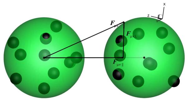
where R_μ is the COM of the cluster μ, as shown in Fig. 1. The radius of gyration R_g is a natural measure of the cluster size. Although the LJ particles may wander across the cluster surfaces, the constraint associates the constituent particles with a specific cluster, so that the dynamic properties of the clusters can be evaluated [19]. It defines the inner number density of the atomistic particles inside each cluster,

$${\rho }_{inner}=N_c∕\frac{4}{3}\pi R_g^3.$$ (9)

The system was simulated in a NVT ensemble with the Nose-Hoover thermostat and the RATTLE algorithm to deal with the constraints [25,26]. The time step was varied from 5×10⁻⁴ to 10⁻³.

FIG. 1.

(Color online) A sketch of the force between two clusters. Small spheres represent atomistic particles while shells represent CG particles. The force vectors drawn in the figure correspond to the instantaneous forces obtained from the MD simulation. The total force F_μν between two clusters is generally not parallel to the radial vector e_μν.

Theoretically, the coarse-grained potential field of the clusters U_CG(R) depends on the K-body configuration {R}≡(R₁, R₂, …, R_K, ρ_c, T), as does the average force 〈F_μ〉_ΓS on cluster μ, which is difficult to evaluate directly. If we approximate the mean-field force on a single cluster by pairwise forces with respect to other clusters [19], 〈F_μ〉_ΓS can be simplified as Σ_ν≠μ〈f(R_μν)〉, where 〈f(r)〉 is the average pair force between two clusters and can be obtained by the MD simulation with specific cluster density ρ_c and temperature k_BT. (We note, however, that this assumption may lead to erroneous results at high densities, as we will discuss later in Sec. IV.) To compute the average pair force 〈f(r)〉, we divide the distance between two clusters into several bins with dr as the distance between each bin. Then, 〈f(r)〉 is obtained by taking the ensemble average of the radial component of the instantaneous force f_μν between two clusters μ and ν, over all microscopic configurations with the pair distance between r−dr/2 and r+dr/2, i.e.,

$$\langle f\left(r\right)\rangle ={\langle {\mathbf{f}}_{\mu \nu }\cdot \frac{{\mathbf{R}}_{\mu \nu }}{R_{\mu \nu }}\rangle }_{r-dr∕2<R_{\mu \nu }<r+dr∕2}.$$ (10)

We also introduce the corresponding pair potential of mean force 〈V(r)〉 as the spatial integration of 〈f(r)〉, i.e.,

$$\langle V\left(r\right)\rangle ={\int }_r^{\infty }\langle f\left(r^{\prime }\right)\rangle d{r}^{\prime }$$ (11)

From the simulations, we found that the average force (potential) field depends on the temperature k_BT, the radius of gyration R_g, the number of particle within each cluster N_c, and the number density of the clusters ρ_c. We discuss our findings in detail below.

B. Simulation results

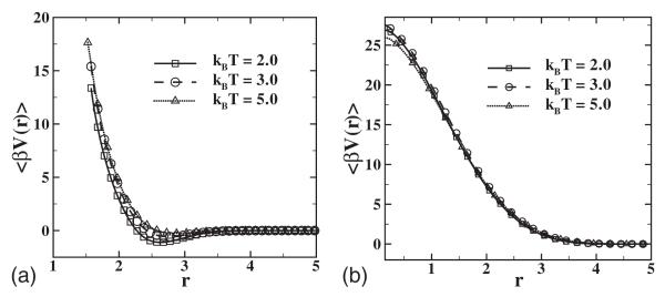
We examine the average pair force 〈f(r)〉 for two different values R_g=0.95 and 1.4397 (the latter value is chosen so that ρinner ≡ρ=0.8). Figure 2 shows the temperature-scaled pair potential β〈V(r)〉 for ρ_c=0.08 and N_c=10. Compared to the LJ system, the CG potential field for both R_g values show softer and temperature-dependent properties. For R_g=1.4397, the potential field is similar to the Gaussian chain model [18]. For R_g=0.95, the clusters behave more like a “single” LJ particle and therefore the force field is stiffer with a stronger repulsive force and deeper attractive well. With temperature between 2.0 and 5.0, both force fields collapse approximately onto a single curve; this property will be discussed further in conjunction with the results of static properties later in this section.

FIG. 2.

Potential of the average pair force scaled by temperature, with ρ=0.8, N_c=10, R_g=0.95 (a), and R_g=1.4397 (b).

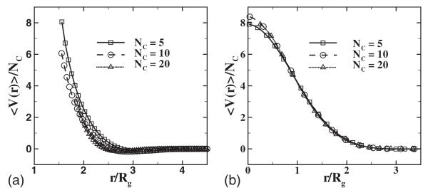
We also examine the potential field with different numbers of particle per cluster N_c, whereas the inner density ρ_inner is the same that at N_c=10 by choosing the proper value of R_g. Similar temperature dependence is observed. Moreover, if we scale the potential by N_c and the distance by R_g, the potential functions approximately collapse into a single curve, as shown in Fig. 3. Based on the results we obtained, we can propose the following scaling:

$$\begin{array}{cc}\hfill \langle f\left(r\right)\rangle & ~\frac{N_c{k}_{B}T}{R_g}h(r∕R_g),\hfill \\ \hfill \langle V\left(r\right)\rangle & ~N_c{k}_B{T}_g(r∕R_g),\hfill \end{array}$$ (12)

where h(r)=−dg(r)/dr and g(r) are dimensionless functions depending on ρ_c and ρ_inner. Note that these simulation results are similar to the scaling relationship for an unconstrained DPD system as derived in [27].

FIG. 3.

Potential of the average pair force scaled by N_c with k_BT=3.0, ρ=0.8, N_c=10, R_g=0.95 (a), and R_g=1.4397 (b).

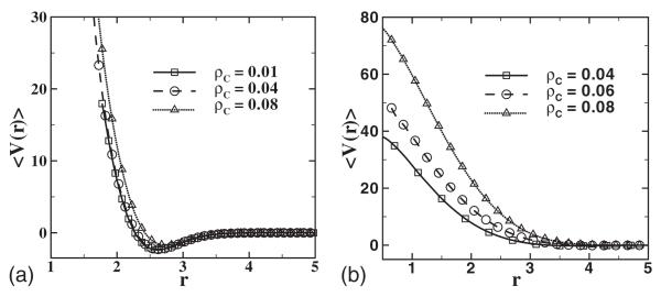
Figure 4 shows 〈f(r)〉 for different number densities ρ_c at fixed temperature k_BT=3.0. Compared with the R_g=0.95 case, 〈f(r)〉 for R_g=1.4397 depends strongly on ρ_c, indicating a significant many-body effect, which may affect the properties of the coarse-grained system, as discussed in Sec. IV.

FIG. 4.

Potential of the average pair force for different densities with N_c=10, k_BT=3.0, R_g=0.95 (a), and R_g=1.4397 (b).

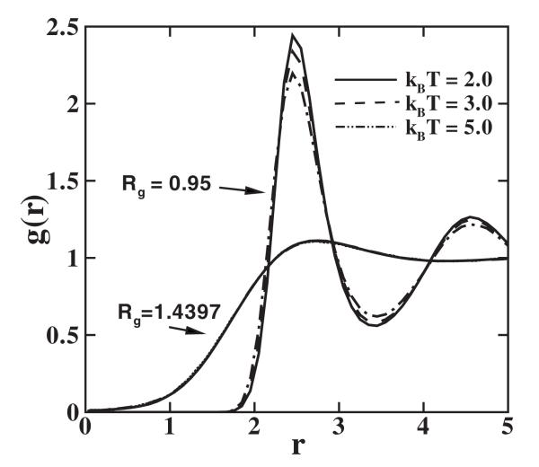
Having obtained the CG force field, we now turn to the static and dynamic properties of the system. Figure 5 shows the radial distribution function g(r) of the clusters at different temperatures. For R_g=1.4397, g(r) is flat and similar to the standard DPD result, while for R_g=0.95, g(r) is much sharper, similar to the single LJ particle result as expected. Unlike the simple fluid system, the radial distribution function shows very weak dependence on temperature between 2.0 and 5.0. This result can be readily understood from the weak temperature dependence of 〈V(r)〉 shown in Fig. 2.

FIG. 5.

Radial distribution function g(r) computed for different temperatures, with ρ=0.8, N_c=10, R_g=0.95, and R_g=1.4397. For the latter case, the three curves coincide.

For dynamic properties, we determine the self-diffusivity of the clusters in the MD system by the Einstein relationship

$$D=\underset{t\to \infty }{\lim }\frac{1}{6t}\langle {\mid {\mathbf{R}}_{\mu }\left(t\right)-{\mathbf{R}}_{\mu }\left(0\right)\mid }^2\rangle .$$ (13)

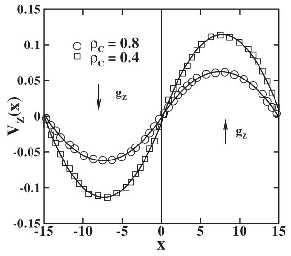
We determine the viscosity of the MD system by the periodic Poiseuille flow method [28] and Lees-Edwards Couette flow. The velocity profile obtained for the periodic Poiseuille flow is shown in Fig. 6. For simulation details, we refer to [28]. The dynamic properties are listed in Table I.

FIG. 6.

Velocity profiles obtained using the periodic Poiseuille flow method. The square and circle symbols represent velocity profiles for ρ=0.8 and 0.4, respectively. The lines are quadratic fit curves for each case. The body force g_z is added on each atomistic particle; g_z is chosen as 0.02 and 0.005 for ρ=0.8 and 0.4, respectively. The box size is changed to 30×15×15 in this test and the temperature is k_BT=3.0.

TABLE I.

Dynamic properties for the MD system with k_BT=3.0 and N_c=10; D, η, and S_c stand for diffusivity, dynamic viscosity, and Schmidt number, respectively.

ρ	Rg	D	η	Sc
0.8	0.95	0.0234	7.41	395
0.4	0.95	0.271	1.05	9.69
0.8	1.4397	0.0255	7.08	347
0.4	1.4397	0.141	1.66	29.4

IV. COARSE-GRAINED MODELS

To investigate the relationship between the two different scales we construct different mesoscale models based on the microscopic results in the previous section. Specifically, we construct CG clusters whose mass is the sum of the masses of MD particles within each cluster. The CG system remains in the canonical ensemble at the same temperature k_BT.

A. Mean force field approach

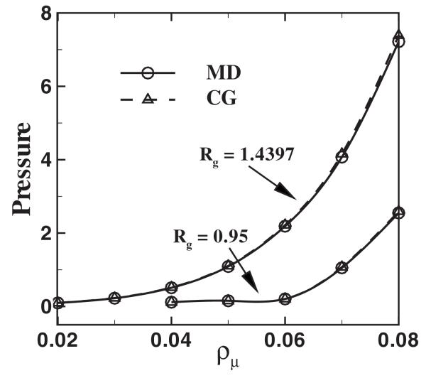
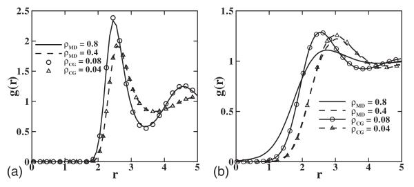
We start with a very simple model where we employ only the average force field, i.e., the first term in Eq. (1). The static properties are determined by this term. Figure 7 compares the equation of state (EOS) of the CG system with the MD system. The results are close to the MD results with a difference less than 2%. Figure 8 compares the radial distribution function of the system. For R_g=0.95, the results of the MD and CG systems match well over the entire density regime. However, for R_g=1.4397 and ρ_c=0.08, the CG result shows a sharper peak than the MD result. Similar differences have been reported for flexible polymer chains in [20,22]. In contrast, Akkermans and Briels [29] proposed a structure-based effective potential which reproduces the radial distribution of coarse-grained polymer system over the entire density regime. However, it generates a pressure much lower than the MD system. These differences are primarily due to the approximation of the clusters as point particles and the absence of the full many-body interaction, which plays an important role at high density and larger R_g.

FIG. 7.

Pressure computed by MD and CG simulations for N_c=10 and k_BT=3.0 with R_g=0.95 and 1.4397.

FIG. 8.

Radial distribution function g(r) of the coarse-grained particles for ρ_c=0.08 and 0.04, with R_g=0.95 (a) and 1.4397 (b). The lines denote the MD simulation results. The symbols correspond to MD simulations.

In general, the mean field by itself cannot reproduce the correct dynamic properties of the CG system. As an illustration, we calculate the self-diffusion coefficient and the dynamic viscosity for CG system of R_g=1.4397 with ρ_c=0.08 and k_BT=3.0. The results are D_MF=0.53 and η_MF=0.74, respectively, indicating a larger mass transport and a smaller momentum transport, compared with the MD system (D_MD=0.0255, η_MD=7.08). Moreover, this discrepancy cannot be eliminated by simply rescaling the units of the CG system. Specifically, if we artificially match the diffusivity of two system by rescaling the time unit of the CG system, while keeping the length and mass units fixed, the scaled time unit of CG system is [t]_MF=20.78[t]_MD. Consequently, the dynamic viscosity of the CG system, by the mean-field model, should be 0.74[M]/[L][t]_MF=0.0356[M]/[L][t]_MD, which is different from the MD result η_MD=7.08. In particular, the dimensionless Schmidt number is different in the two systems. In the MD system, S_cMD is around 347 (see Table I) while in the mean field S_cMF is around 1. Therefore, the dissipative and random force terms in Eq. (1) cannot be neglected if the dynamic properties are considered.

B. Langevin thermostat approach

Next, we discuss a model including the dissipative and random force terms. We assume that each component of the random force on a CG particle is identical independently distributed (i.i.d.); hence, Eqs. (3) and (4) are simplified, respectively, as

$$\langle \left[\delta {\mathbf{F}}_{\mu }^{\mathcal{Q}}\right(t\left)\right]{\left[\delta {\mathbf{F}}_{\nu }^{\mathcal{Q}}\right(0\left)\right]}^T\rangle ={\sigma }^2{\delta }_{\mu \nu }\delta \left(t\right)I,$$ (14)

$$\beta {\int }_0^{t}ds\langle \left[\delta {\mathbf{F}}_{\mu }^{\mathcal{Q}}\right(t-s\left)\right]{\left[\delta {\mathbf{F}}_{\nu }^{\mathcal{Q}}\right(0\left)\right]}^T\rangle \cdot {\mathbf{V}}_{\nu }\left(s\right)=\gamma {\delta }_{\mu \nu }{\mathbf{V}}_{\nu }\left(t\right),$$ (15)

where I is the identity matrix and γ=βσ²/2 is defined as the friction coefficient. The fluctuation-dissipation theorem is satisfied and Eq. (1) simplifies to

$${\stackrel{.}{\mathbf{P}}}_{\mu }=\sum _{\nu \ne \mu }\langle f\left(r_{\mu \nu }\right)\rangle {\mathbf{e}}_{\mu \nu }-\gamma {\mathbf{V}}_{\nu }+\delta {\mathbf{F}}_{\mu }^{\mathcal{Q}},$$ (16)

where V_μ is the velocity of the CG particle. This model states that the motion of the CG particles is coupled with the standard Langevin thermostat [1,30], as implemented in the coarse-grained polymer melts [6]. Note that the friction coefficient γ is not casually chosen but computed by Eq. (15).

The instantaneous random force term on a single cluster μ is $\delta {\mathbf{F}}_{\mu }^{\mathcal{Q}}={\mathbf{F}}_{\mu }-\langle {\mathbf{F}}_{\mu }\rangle$, where 〈F_μ〉 is a function depending on K-body configurations of the system, which is difficult to evaluate directly. In practice, we approximate 〈F_μ〉 by decomposing it into pairwise functions as discussed in Sec. III A. Accordingly, we approximate $\delta {\mathbf{F}}_{\mu }^{\mathcal{Q}}$ as

$$\delta {\mathbf{F}}_{\mu }^{\mathcal{Q}}\approx \sum _{\nu \ne \mu }\delta {\mathbf{f}}_{\mu \nu }^{\mathcal{Q}},$$ (17)

where $\delta {\mathbf{f}}_{\mu \nu }^{\mathcal{Q}}$ is the pairwise random force between clusters μ and ν, defined as

$$\delta {\mathbf{f}}_{\mu \nu }^{\mathcal{Q}}={\mathbf{f}}_{\mu \nu }-\langle f\left(r\right)\rangle {\mathbf{e}}_{\mu \nu },$$ (18)

where f_μν is the instantaneous force between the two clusters.

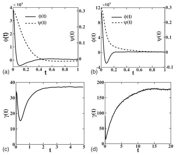
Figure 9 shows the correlation function of the random force on a single cluster. It also verifies the Markovian approximation in Eq. (4) since the autocorrelation of velocity decays slower than the random force correlation. The friction coefficient is obtained by taking the long-time integration of the random force correlation function until a converged value is obtained.

FIG. 9.

Computation of the Langevin thermostat coefficient. (a) and (b) Time correlation of the velocity and random force on each cluster for ρ=0.8, N_c=10, and k_BT=3.0. The left axis $\varphi \left(t\right)=\langle \delta F_{\mu x}^{\mathcal{Q}}\left(t\right)\delta F_{\mu x}^{\mathcal{Q}}\left(0\right)\rangle$ denotes the time correlation of the x-component of total random force on a cluster. The right axis ψ(t)=〈v_x(0)v_x(t)〉 denotes the x-component of the velocity correlation of a cluster. (c) and (d) Time integration of correlation defined by $\gamma \left(t\right)=\beta {\int }_0^t\langle \delta F_{\mu x}^{\mathcal{Q}}(t-s)\delta F_{\mu x}^{\mathcal{Q}}\left(0\right)\rangle ds$. The result converges when t≈3.0 for R_g=0.95 and t≈15.0 for R_g=1.4397.

Having obtained the friction coefficient, we are ready to simulate the CG system by Eq. (16) using the standard algorithm [26]. The temperature is kept constant by the Langevin thermostat and the static properties are determined by the mean force term as shown in the previous section. For R_g=0.95 and ρ_c=0.08 (ρ=0.8), the self-diffusion coefficient determined by this method is D_LD=0.0063, which is approximately four times smaller than the MD result (D_MD=0.0234)(see Table I).

Moreover, this CG system does not capture the correct hydrodynamics. This result originates from Eq. (14), which assumes that the random force on each CG particle is inde-pendent and therefore cannot be represented in a pairwise fashion. Physically, it appears that each CG particle is surrounded by some heat bath particles [31], and the random force on each particle arises from thermal collisions with heat bath particles. Therefore, the momentum transport between two clusters in the MD system is modeled in two parts: the pairwise interaction between the two CG particles through the mean force field and the thermal collisions with the heat bath particles represented as the i.i.d. force $\delta {\mathbf{F}}^{\mathcal{Q}}$ on each particle. Specifically, if the conservative interaction is much larger than the thermal collision effect, the system approaches the Newtonian regime [32]. However, if the friction and random forces become comparable with the conservative force (as in the case of this study), the Langevin thermostat significantly damps the hydrodynamic correlation [31] between the particles, and the system cannot reproduce the correct hydrodynamics [32,33]. In this study, the loss of momentum transport between the CG particles in the random force field eliminates the information needed for the calculation of viscosity.

C. DPD

To establish the correlation of the random force between different CG clusters, we decompose the random force into additive pairwise components between different particles. Generally, the random force $\delta {\mathbf{f}}_{\mu \nu }^{\mathcal{Q}}$ defined by Eq. (18) is not along the radial direction e_μν, as shown in Fig. 1. Therefore, we decompose $\delta {\mathbf{f}}_{\mu \nu }^{\mathcal{Q}}$ into two parts: the radial force along e_μν and the perpendicular part, e.g.,

$$\begin{array}{cc}\hfill \delta {\mathbf{f}}_{\mu \nu }^{\mathcal{Q}}& =\left({\mathbf{e}}_{\mu \nu }{\mathbf{e}}_{\mu \nu }^T\right)\cdot \delta {\mathbf{f}}_{\mu \nu }^{\mathcal{Q}}+(I-{\mathbf{e}}_{\mu \nu }{\mathbf{e}}_{\mu \nu }^T)\cdot \delta {\mathbf{f}}_{\mu \nu }^{\mathcal{Q}}\hfill \\ \hfill & =\delta f_{\mu \nu ,\parallel }^{\mathcal{Q}}{\mathbf{e}}_{\mu \nu }+\delta {\mathbf{f}}_{\mu \nu ,\perp }^{\mathcal{Q}},\hfill \end{array}$$ (19)

where $\delta {\mathbf{f}}_{\mu \nu ,\perp }^{\mathcal{Q}}$ is the perpendicular part of the random force. We assume that the random force pairs are independent and uncorrelated in time, i.e.,

$$\begin{array}{cc}\hfill \langle \delta f_{\mu \nu ,\parallel }^{\mathcal{Q}}\left(t\right)\delta f_{∊\eta ,\parallel }^{\mathcal{Q}}\left(0\right)\rangle & ={\left[{\sigma }_{\parallel }{w}_{\parallel }\right(R\left)\right]}^2\mathcal{K}\left(t\right),\hfill \\ \hfill \langle \delta {\mathbf{f}}_{\mu \nu ,\perp }^{\mathcal{Q}}\left(t\right)\cdot \delta {\mathbf{f}}_{∊\eta ,\perp }^{\mathcal{Q}}\left(0\right)\rangle & =2{\left[{\sigma }_{\perp }{w}_{\perp }\right(R\left)\right]}^2\mathcal{K}\left(t\right),\hfill \end{array}$$ (20)

where σ_∥w_∥(R) and σ_⊥w_⊥(R) are the variances of the random force depending on the distance R, and

$$\mathcal{K}\left(t\right)=({\delta }_{\mu ∊}{\delta }_{\nu \eta }+{\delta }_{\mu \eta }{\delta }_{\nu ∊})\delta \left(t\right).$$ (21)

These assumptions lead to

$$\langle \delta {\mathbf{f}}_{\mu \nu }^{\mathcal{Q}}\left(t\right)\delta {\mathbf{f}}_{∊\eta }^{\mathcal{Q}}{\left(0\right)}^T\rangle =({\delta }_{\mu ∊}{\delta }_{\nu \eta }-{\delta }_{\mu \eta }{\delta }_{\nu ∊})\times \langle \delta {\mathbf{f}}_{\mu \nu }^{\mathcal{Q}}\left(t\right)\delta {\mathbf{f}}_{\mu \nu }^{\mathcal{Q}}{\left(0\right)}^T\rangle .$$ (22)

In addition, the memory kernel ${\int }_0^{\infty }\langle \delta {\mathbf{f}}_{\mu \nu }^{\mathcal{Q}}\left(t\right)\delta {\mathbf{f}}_{\mu \nu }^{\mathcal{Q}}{\left(0\right)}^T\rangle dt$ is isotropic in planes perpendicular to e_μν. Therefore, we decompose the matrix as

$$\begin{array}{cc}\hfill {\gamma }_{\mu \nu }& =\beta {\int }_0^{\infty }\langle \delta {\mathbf{f}}_{\mu \nu }^{\mathcal{Q}}\left(t\right)\delta {\mathbf{f}}_{\mu \nu }^{\mathcal{Q}}{\left(0\right)}^T\rangle dt\hfill \\ \hfill & ={\gamma }_{\parallel }\left(R_{\mu \nu }\right){\mathbf{e}}_{\mu \nu }{\mathbf{e}}_{\mu \nu }^T+{\gamma }_{\perp }\left(R_{\mu \nu }\right)(I-{\mathbf{e}}_{\mu \nu }{\mathbf{e}}_{\mu \nu }^T),\hfill \end{array}$$ (23)

where γ_∥ and γ_⊥ are scalars depending on R_μν. Using Eq. (20), they are determined by

$$\begin{array}{cc}\hfill {\gamma }_{\parallel }\left(R_{\mu \nu }\right)={\mathbf{e}}_{\mu \nu }^T{\gamma }_{\mu \nu }\mathbf{e}\mu \nu & =\beta {\int }_0^{\infty }dt\langle \delta f_{\mu \nu ,\parallel }^{\mathcal{Q}}\left(t\right)\delta f_{\mu \nu ,\parallel }^{\mathcal{Q}}\left(0\right)\rangle \hfill \\ \hfill & =\frac{1}{2}\beta {\left[{\sigma }_{\parallel }{w}_{\parallel }\right(R_{\mu \nu }\left)\right]}^2,\hfill \end{array}$$ (24)

$$\begin{array}{cc}\hfill {\gamma }_{\perp }\left(R_{\mu \nu }\right)& =\frac{1}{2}\mathrm{Tr}\left[\right(I-{\mathbf{e}}_{\mu \nu }{\mathbf{e}}_{\mu \nu }^T\left){\gamma }_{\mu \nu }\right(I-{\mathbf{e}}_{\mu \nu }{\mathbf{e}}_{\mu \nu }^T\left)\right]\hfill \\ \hfill & =\frac{1}{2}\beta \mathrm{Tr}\left[{\int }_0^{\infty }\langle (I-{\mathbf{e}}_{\mu \nu }{\mathbf{e}}_{\mu \nu }^T)\delta {\mathbf{f}}_{\mu \nu }^{\mathcal{Q}}\left(t\right)\delta {\mathbf{f}}_{\mu \nu }^{\mathcal{Q}}{\left(0\right)}^T\times (I-{\mathbf{e}}_{\mu \nu }{\mathbf{e}}_{\mu \nu }^T)\rangle dt\right]\hfill \\ \hfill & =\frac{1}{2}\beta {\int }_0^{\infty }\langle \delta {\mathbf{f}}_{\mu \nu ,\perp }^{\mathcal{Q}}\left(t\right)\cdot \delta {\mathbf{f}}_{\mu \nu ,\perp }^{\mathcal{Q}}\left(0\right)\rangle dt\hfill \\ \hfill & =\frac{1}{2}\beta {\left[{\sigma }_{\perp }{w}_{\perp }\right(R_{\mu \nu }\left)\right]}^2.\hfill \end{array}$$ (25)

The dissipative force on a single cluster μ is then obtained from

$$\begin{array}{cc}\hfill \beta \sum _{\eta }{\int }_0^{\infty }ds\langle {\mathbf{F}}_{\mu }^{\mathcal{Q}}\left(s\right){\mathbf{F}}_{\eta }^{\mathcal{Q}}{\left(0\right)}^T\rangle \cdot {\mathbf{V}}_{\eta }& =\beta \sum _{\eta }\sum _{\nu \ne \mu }\sum _{∊\ne \eta }{\int }_0^{\infty }ds\langle {\mathbf{f}}_{\mu \nu }^{\mathcal{Q}}\left(s\right){\mathbf{f}}_{\eta ∊}^{\mathcal{Q}}{\left(0\right)}^T\rangle \cdot {\mathbf{V}}_{\eta }\hfill \\ \hfill & =\sum _{\eta }\sum _{\nu \ne \mu }\sum _{∊\ne \eta }({\delta }_{\mu \eta }{\delta }_{\nu ∊}-{\delta }_{\mu ∊}{\delta }_{\nu \eta })\left[{\gamma }_{\parallel }\right(R_{\mu \nu }){\mathbf{e}}_{\mu \nu }{\mathbf{e}}_{\mu \nu }^T+{\gamma }_{\perp }(R_{\mu \nu })\times (I-{\mathbf{e}}_{\mu \nu }{\mathbf{e}}_{\mu \nu }^T\left)\right]\cdot {\mathbf{V}}_{\eta }\hfill \\ \hfill & =\sum _{\nu \ne \mu }{\gamma }_{\parallel }\left(R_{\mu \nu }\right){\mathbf{e}}_{\mu \nu }{\mathbf{e}}_{\mu \nu }^T\cdot ({\mathbf{V}}_{\mu }-{\mathbf{V}}_{\nu })+\sum _{\nu \ne \mu }{\gamma }_{\perp }\left(R_{\mu \nu }\right)(I-{\mathbf{e}}_{\mu \nu }{\mathbf{e}}_{\mu \nu }^T)\cdot ({\mathbf{V}}_{\mu }-{\mathbf{V}}_{\nu })\hfill \\ \hfill & =\sum _{\nu \ne \mu }{\gamma }_{\parallel }\left(R_{\mu \nu }\right)\times ({\mathbf{e}}_{\mu \nu }\cdot {\mathbf{V}}_{\mu \nu }){\mathbf{e}}_{\mu \nu }+\sum _{\nu \ne \mu }{\gamma }_{\perp }\left(R_{\mu \nu }\right)[{\mathbf{V}}_{\mu \nu }-({\mathbf{e}}_{\mu \nu }\cdot {\mathbf{V}}_{\mu \nu }\left){\mathbf{e}}_{\mu \nu }\right].\hfill \end{array}$$ (26)

Similar to Eq. (4), the above approximation replaces the continuously varying impulses on a CG particle by discrete time-independent values, along both the radial and perpendicular directions for each pair. The first term on the righthand side of the above equation is the dissipative force of standard DPD [5,15,34]. The second term represents the friction between two CG particles along the perpendicular directions. This is exactly the dissipative force for the “transverse DPD thermostat,” recently proposed by Junghans et al. [35]. Putting the three terms together, we obtain the generalized DPD equation:

$${\stackrel{.}{\mathbf{P}}}_{\mu }=\sum _{\nu \ne \mu }\langle f\left(r_{\mu \nu }\right)\rangle {\mathbf{e}}_{\mu \nu }-\sum _{\nu \ne \mu }{\gamma }_{\parallel }\left(R_{\mu \nu }\right)({\mathbf{e}}_{\mu \nu }\cdot {\mathbf{V}}_{\mu \nu }){\mathbf{e}}_{\mu \nu }+\sum _{\nu \ne \mu }{\gamma }_{\perp }\left(R_{\mu \nu }\right)[\mathbf{V}\mu \nu -({\mathbf{e}}_{\mu \nu }\cdot {\mathbf{V}}_{\mu \nu }\left){\mathbf{e}}_{\mu \nu }\right]+\sum _{\nu }\delta {\mathbf{f}}_{\mu \nu }^{\mathcal{Q}}.$$ (27)

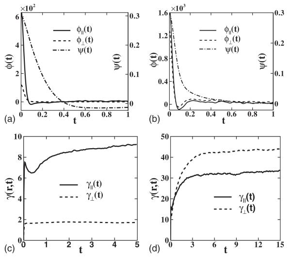
Specifically, we use Eqs. (24) and (25) to calculate the friction coefficient in the radial and perpendicular directions, with $\delta f_{\mu \nu ,\parallel }^{\mathcal{Q}}$ and $\delta {\mathbf{f}}_{\mu \nu ,\perp }^{\mathcal{Q}}$ defined by Eq. (19). Noting that the radial vector e_μν changes with time, the random force terms $\delta f_{\mu \nu ,\parallel }^{\mathcal{Q}}\left(t\right)$ and $\delta f_{\mu \nu ,\perp }^{\mathcal{Q}}\left(t\right)$ are defined by projecting $\delta {\mathbf{F}}_{\mu \nu }^{\mathcal{Q}}\left(t\right)$ onto the vector e_μν at time zero. Figures 10(a) and 10(b) show the random force correlation along both the parallel and perpendicular directions. For R_g=0.95, the clusters behave like the single particles, and the radial part of random force dominates for most distances. However, for the larger R_g=1.4397, the shearing part becomes comparable to the radial part, and the integration converges for longer times, as shown in Fig. 10(d).

FIG. 10.

(a) The left axis denotes the time correlation of the pairwise random force between two clusters for ρ=0.8, N_c=10, k_BT=3.0, (a) R_g=0.95, r=2.65, and (b) R_g=1.4397, r=2.25. ϕ_∥(t) and ϕ_⊥(t) denote the radial and the perpendicular parts of the correlation, respectively. The right axis ψ(t) denotes the velocity correlation function, which decays slower than the random force as shown. Bottom: time integration of the correlation function with (c) R_g=0.95, r=2.65 and (d) R_g=1.4397, r=2.25.

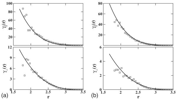
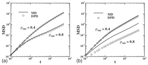
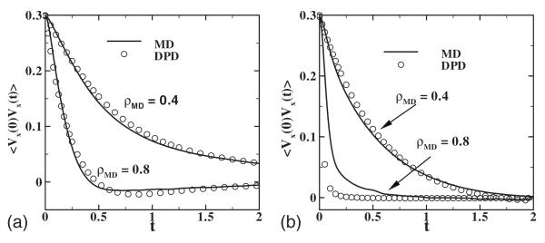
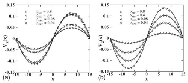
Figure 11 shows the friction coefficients for different distances with R_g=0.95 and k_BT=3.0. We fit γ_∥ and γ_⊥ by polynomials a(1.0-r/b)ⁿ, where n is 4.0 and 3.0, respectively. Using the fitted function form of γ, we simulate the CG system by DPD using both the radial and the shear thermostats [35]. In Figs. 12 and 13, we show the mean-square displacement of the CG system in the long-time region and the velocity correlations in short-time region. The difference in the results obtained with the best fit and the original points is less than 5%. Figure 14 shows velocity profiles from both the MD and DPD systems obtained by the periodic Poiseuille flow method. As the momentum transport between clusters is represented by pairwise forces, the simulation results recover Newtonian flow behavior in this model, as expected. The dynamic properties of the DPD system are listed in Table II.

FIG. 11.

Radial and shear friction coefficients for R_g=0.95; the solid line is a fit to (a) ρ_c=0.08, γ_∥(r)=a(1-r/b)⁴, where a=1.06 ×10³, b=3.6; γ_⊥(r)=a(1-r/b)³, where a=80.1, b=3.5 and (b) ρ_c=0.08, γ_∥(r)=a(1-r/b)⁴, where a=0.97×10³, b=3.6, ρ=0.4; γ_⊥(r)=a(1-r/b)³, where a=35.6, b=3.5.

FIG. 12.

Mean-square displacement (scaled by 6.0) of the clusters and CG particles for different densities with R_g=0.95 (a) and R_g=1.4397 (b); N_c=10 and k_BT=3.0.

FIG. 13.

Velocity correlation function of the clusters and CG particles for different densities with R_g=0.95 (a) and R_g=1.4397 (b); N_c=10 and k_BT=3.0.

FIG. 14.

Velocity profile for periodic Poiseuille flow method for MD and DPD models. The solid line is the quadratic fit to the numerical results. Body forces f_MD and f_CG are applied on each MD and CG particle, respectively. Top: R_g=0.95, ρ=0.4, f_MD=0.005, f_CG=0.05; R_g=0.95, ρ=0.8, f_MD=0.02, f_CG=0.2. (b) R_g=1.4397, ρ=0.4, f_MD=0.01, f_CG=0.1; R_g=1.4397, ρ=0.8, f_MD=0.02, f_CG=0.4.

TABLE II.

Dynamic properties for MD and CG systems with k_BT=3.0 and N_c=10.

	Rg	D	η	Sc
ρ =0.8	0.95	0.0234	7.41	395
ρDPD=0.08	0.95	0.0195	9.69	621
ρ =0.4	0.95	0.271	1.05	9.69
ρDPD=0.04	0.95	0.269	1.075	9.98
ρ =0.8	1.4397	0.0255	7.08	347
ρDPD=0.08	1.4397	0.00525	41.23	9.81×103
ρ =0.4	1.4397	0.141	1.66	29.4
ρDPD=0.04	1.4397	0.133	2.26	42.47

The DPD results show smaller diffusivities and larger viscosities compared with the MD results, with the deviations being different for the four cases. For R_g=0.95, the difference of the diffusivity is about 16% and 1.2% for DPD densities ρ_c=0.08 and 0.04, respectively. For R_g=1.4397, the difference is about 80% and 25%, respectively. The differ-ences are due mainly to two factors: the Markovian approximation and the overestimation of the friction coefficient. First, the DPD model we have derived is based on the assumption that the velocity correlation of the CG particles decays more slowly than the random force correlation. When the density is high and the velocity correlation is comparable to the random force correlation, the DPD particles would be overdamped (see Ref. [14]), which explains why we get better results in the semidilute regime. Second, the friction coefficient we use is overestimated since we lack the “full” information of the force field for the CG system [36]. Physically, the many-body potential field U_CG(R^K) is the mean field which minimizes the random force covariance. It depends on the entire particle configuration of the CG system. Therefore, the pairwise mean force field implemented in this study would always lead to overestimated friction coefficients. In this study, when the many-body effect is important (e.g., R_g=1.4397 and ρ=0.8; see Fig. 4), γ(r) is largely overestimated in this pairwise style and the diffusivity of the DPD system is only 20% of the MD results. For the other three cases, the many-body effect is less important and the pairwise mean field we use can approximate U_CG(R^K). The friction coefficient can be accurately estimated and therefore the DPD results match reasonably well with the MD results.

V. OTHER POTENTIALS

As shown in the previous sections, while the mean force field 〈f(r)〉 we chose reproduces the EOS in a wide density range, it does not reproduce the structure properties of the MD system in the high-density regime when R_g is large. On the other hand, several methods [18,29,37,38] have been proposed for obtaining a structure-based effective potential V_eff(r), which reproduces the pair distribution function of the MD system. Therefore, it is worthwhile exploring if a structure-based force field can improve the dynamic property predictions.

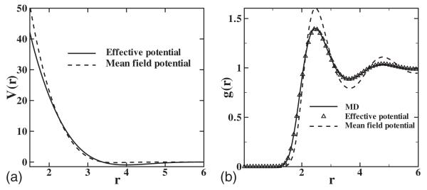
For demonstration, we compute the pair distribution function by MD simulation with R_g=1.2 and ρ=0.8. An iterative method [37] is used to obtain V_eff(r), where 〈V(r)〉 is used as the initial guess. As shown in Fig. 15, V_eff(r) shows a longer attractive tail compared with the mean-field result, and it reproduces the pair distribution function. However, the pressure obtained is 5.37, which is approximately 18% lower than the MD result. In contrast, with our approach EOS is reproduced very accurately.

FIG. 15.

(a) Effective potential V_eff(r) obtained from the pair distribution function of MD simulation and mean-field potential 〈V(r)〉 obtained from Eq. (10) with R_g=1.2, k_BT=3.0, N_c=10, and ρ=0.8. V_eff(r) shows an artificially longer tail compared with 〈V(r)〉. (b) Pair distribution function measured by MD, V_eff(r), and 〈V(r)〉.

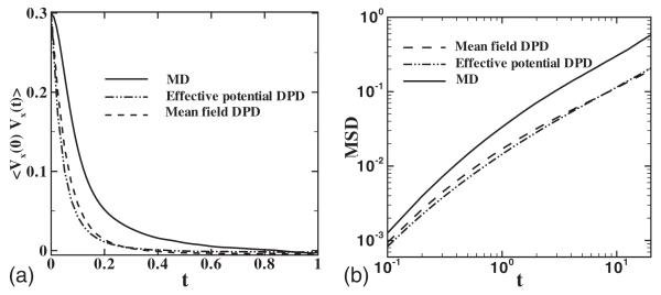
Next, V_eff(r) is used as the input for Eqs. (24) and (25) to compute the dissipative force term and the dynamic properties of the CG system are revisited. As shown in Fig. 16, both the velocity correlation and mean-square displacement obtained from V_eff(r) show smaller values than the MD results. No obvious improvement is observed compared with the mean-field results. This result is reasonable and consistent with what we expect. Although the pairwise effective potential V_eff(r) can mimic the higher-order interactions of the MD system and can reproduce the second-order correlation (radial distribution function)(as shown in Fig. 15), the higher-order correlations of the MD system may not be reproduced. The instantaneous random forces $\delta f_{\mu \nu ,\parallel }^{\mathcal{Q}}\left(t\right)$ and $\delta f_{\mu \nu ,\perp }^{\mathcal{Q}}\left(t\right)$ in Eqs. (24) and (25) may still be far away from the real value, depending on the strength of the higher-order correlation of the MD system.

FIG. 16.

Velocity correlation function (a) and mean-square displacement (b)(scaled by 6.0) measured by MD, effective potential V_eff(r), and mean-field potential 〈V(r)〉 for R_g=1.2, k_BT=3.0, N_c=10, and ρ=0.8.

Finally, we also checked the coarse-graining results with the Weeks-Chandler-Andersen potential as the input interaction between the MD particles. Both static and dynamic properties show qualitatively similar results with the previous sections, e.g., we can represent the MD clusters by DPD particles and predict the friction coefficient reasonably well in semidilute regime or R_g relatively small, which indicates that the approach we use is quite general and may be extended to many other systems.

VI. SUMMARY AND DISCUSSION

Starting from a microscopic simulation of LJ clusters in a canonical ensemble, we conducted mesoscopic simulations of the system by coarse-graining clusters that we constructed with a fixed radius of gyration and represented them as point particles. The mean, dissipative, and random forces needed for the motion of the CG particles are extracted from the microscopic simulation. In particular, the mean force field is approximated by the ensemble average of the pairwise atomistic force between two clusters, and we find that its corresponding potential is proportional to the number of particles per cluster. We also approximated the memory kernel of the dissipative force with two different assumptions, leading to Langevin dynamics and dissipative particle dynamics (DPD), with the latter endowed with two thermostats. While both models produce the same static properties, the Langevin model requires extra hydrodynamic information as input to produce the correct dynamic properties. On the other hand, DPD seems to be a good candidate for reproducing the correct mass and momentum transport properties. Compared to the MD results, the DPD results can approximate the dynamic properties reasonably well when the many-body effect of microscopic system is not too strong (e.g., for small R_g or semidilute system). However, the DPD model is not so successful when the many-body effect is very strong, i.e., for large density and R_g. We note that we also tested DPD with a single thermostat, i.e., neglecting the perpendicular contribution as it is typically done in standard DPD simulations. In that case, we did not achieve as good in accuracy for the dynamic properties for the small R_g cases as we did with the two-thermostat DPD, but the results for the high R_g cases were slightly better.

This work provides a general framework for constructing a “bottom-up” mesoscopic simulation directly from the microscopic level, with explicit relationships between the two hierarchies. It can be extended to the mesoscopic description of complex fluid systems in the dilute and semidilute regimes, e.g., star polymers, flexible polymer chains, and mixture of polymer and colloid systems. The friction coefficients can be extracted from microscopic sample systems in pilot simulations within affordable computation time. Hence, coarse-grained simulation of a large system at the mesoscopic level can be conducted with the various dynamic properties evaluated directly, i.e., without any scaling ambiguities.

We note, however, that in the present study the friction coefficient was computed with data from equilibrium MD simulations and this may affect the computation of the dynamic viscosity, which was obtained here based on CG simulations of a periodic Poiseuille or Couette flow. It will be interesting in the future to investigate whether improved predictions of the dynamic viscosity can be achieved if the friction coefficients are based on nonequilibrium MD simulations. We also note the similarity of the “parallel-normal” thermostat in the current work with a similar thermostat employed in the single-particle DPD version in [39,40] where a shear drag coefficient is imposed explicitly. In particular, to obtain the correct hydrodynamics in flow past a sphere in [39] it was found that γ_∥=γ_⊥ for the fluid particles, which is consistent with the results obtained here for large R_g, which correspond to large shear contribution.

Another natural extension of this work is to construct friction force models, where a more sophisticated mean force field is implemented in the coarse-grained system. In the high-density regime, the pairwise mean field in this study may not be adequate to describe the full coarse-grained potential field U_CG(R^K), leading to the overestimation of the memory kernel of the dissipative term. In these cases, a mean field that incorporates the “many-body” information may lead to a more accurate dissipative force and therefore more accurate prediction of the dynamic properties.

Finally, rather than a constrained microscopic system, it would be interesting to coarse grain the unconstrained LJ fluid by the DPD model of this study, especially with regard to the computation of the dissipative force term. In this direction, some work has been done in this direction is by Eriksson et al. [23], and also by Flekkøy and Coveney [41]. It would be interesting to directly compute the dissipative force term of the coarse-grained LJ fluid by the method of this study and compare the DPD predictions of dynamic properties with those of the LJ fluid.

References

- [1].Schneider T, Stoll E. Phys. Rev. B. 1978;17:1302. [Google Scholar]
- [2].Lucy LB. Astron. J. 1977;82:1013. [Google Scholar]
- [3].Gingold RA, Monaghan JJ. Mon. Not. R. Astron. Soc. 1977;181:375. [Google Scholar]
- [4].Hoogerbrugge PJ, Koelman J. EPL. 1992;19:155. [Google Scholar]
- [5].Groot RD, Warren PB. J. Chem. Phys. 1997;107:4423. [Google Scholar]
- [6].Padding JT, Briels WJ. J. Chem. Phys. 2001;115:2846. [Google Scholar]
- [7].Lahmar F, Rousseau B. Polymer. 2007;48:3584. [Google Scholar]
- [8].Liew CC, Mikami M. Chem. Phys. Lett. 2003;368:346. [Google Scholar]
- [9].Espanol P. Phys. Rev. E. 1996;53:1572. doi: 10.1103/physreve.53.1572. [DOI] [PubMed] [Google Scholar]
- [10].Zwanzig R. J. Chem. Phys. 1960;33:1338. [Google Scholar]
- [11].Mori H. Prog. Theor. Phys. 1965;33:423. [Google Scholar]
- [12].Vankampen NG, Oppenheim I. Physica A. 1986;138:231. [Google Scholar]
- [13].Silbermann JR, Schoen M, Klapp SHL. Phys. Rev. E. 2008;78:011201. doi: 10.1103/PhysRevE.78.011201. [DOI] [PubMed] [Google Scholar]
- [14].Akkermans RLC, Briels WJ. J. Chem. Phys. 2000;113:6409. [Google Scholar]
- [15].Kinjo T, Hyodo SA. Phys. Rev. E. 2007;75:051109. doi: 10.1103/PhysRevE.75.051109. [DOI] [PubMed] [Google Scholar]
- [16].Espanol P, Serrano M, Zuniga I. Int. J. Mod. Phys. C. 1997;8:899. [Google Scholar]
- [17].Klapp SHL, Diestler DJ, Schoen M. J. Phys.: Condens. Matter. 2004;16:7331. [Google Scholar]
- [18].Louis AA, Bolhuis PG, Hansen JP, Meijer EJ. Phys. Rev. Lett. 2000;85:2522. doi: 10.1103/PhysRevLett.85.2522. [DOI] [PubMed] [Google Scholar]
- [19].Kinjo T, Hyodo S. Mol. Simul. 2007;33:417. [Google Scholar]
- [20].Akkermans RLC, Briels WJ. J. Chem. Phys. 2001;115:6210. [Google Scholar]
- [21].Harmandaris VA, Adhikari NP, van der Vegt NFA, Kremer K. Macromolecules. 2006;39:6708. [Google Scholar]
- [22].Fukunaga H, Takimoto J, Doi M. J. Chem. Phys. 2002;116:8183. [Google Scholar]
- [23].Eriksson A, Jacobi MN, Nystrom J, Tunstrom K. Phys. Rev. E. 2008;77:016707. doi: 10.1103/PhysRevE.77.016707. [DOI] [PubMed] [Google Scholar]
- [24].A point in phase space is , but here we neglect the momentum part.
- [25].Marry V, Ciccotti G. J. Comput. Phys. 2007;222:428. [Google Scholar]
- [26].Allen MP, Tildsley DJ. Computer Simulation of Liquids. Clarendon Press; Oxford: 1987. [Google Scholar]
- [27].Fuchslin RM, Fellermann H, Eriksson A, Ziock H-J. J. Chem. Phys. 2009;130:214102. doi: 10.1063/1.3143976. [DOI] [PubMed] [Google Scholar]
- [28].Backer JA, Lowe CP, Hoefsloot HCJ, Iedema PD. J. Chem. Phys. 2005;122:154503. doi: 10.1063/1.1883163. [DOI] [PubMed] [Google Scholar]
- [29].Akkermans RLC, Briels WJ. J. Chem. Phys. 2001;114:1020. [Google Scholar]
- [30].Kremer K, Grest GS, Carmesin I. Phys. Rev. Lett. 1988;61:566. doi: 10.1103/PhysRevLett.61.566. [DOI] [PubMed] [Google Scholar]
- [31].Dunweg B. J. Chem. Phys. 1993;99:6977. [Google Scholar]
- [32].Pastorino C, Kreer T, Muller M, Binder K. Phys. Rev. E. 2007;76:026706. doi: 10.1103/PhysRevE.76.026706. [DOI] [PubMed] [Google Scholar]
- [33].Soddemann T, Dunweg B, Kremer K. Phys. Rev. E. 2003;68:046702. doi: 10.1103/PhysRevE.68.046702. [DOI] [PubMed] [Google Scholar]
- [34].Espanol P, Warren P. EPL. 1995;30:191. [Google Scholar]
- [35].Junghans C, Praprotnik M, Kremer K. Soft Matter. 2008;4:156. doi: 10.1039/b713568h. [DOI] [PubMed] [Google Scholar]
- [36].Briels WJ, Akkermans RLC. Mol. Simul. 2002;28:145. [Google Scholar]
- [37].Soper AK. Chem. Phys. 1996;202:295. [Google Scholar]
- [38].Lyubartsev AP, Laaksonen A. Phys. Rev. E. 1995;52:3730. doi: 10.1103/physreve.52.3730. [DOI] [PubMed] [Google Scholar]
- [39].Pan W, Pivkin IV, Karniadakis GE. EPL. 2008;84:10012. [Google Scholar]
- [40].Espanol P. Phys. Rev. E. 1998;57:2930. [Google Scholar]
- [41].Flekkøy EG, Coveney PV. Phys. Rev. Lett. 1999;83:1775. [Google Scholar]