A mesoscopic bridging scale method for fluids and coupling dissipative particle dynamics with continuum finite element method

Abstract

A multiscale procedure to couple a mesoscale discrete particle model and a macroscale continuum model of incompressible fluid flow is proposed in this study. We call this procedure the mesoscopic bridging scale (MBS) method since it is developed on the basis of the bridging scale method for coupling molecular dynamics and finite element models [G.J. Wagner, W.K. Liu, Coupling of atomistic and continuum simulations using a bridging scale decomposition, J. Comput. Phys. 190 (2003) 249–274]. We derive the governing equations of the MBS method and show that the differential equations of motion of the mesoscale discrete particle model and finite element (FE) model are only coupled through the force terms. Based on this coupling, we express the finite element equations which rely on the Navier–Stokes and continuity equations, in a way that the internal nodal FE forces are evaluated using viscous stresses from the mesoscale model. The dissipative particle dynamics (DPD) method for the discrete particle mesoscale model is employed. The entire fluid domain is divided into a local domain and a global domain. Fluid flow in the local domain is modeled with both DPD and FE method, while fluid flow in the global domain is modeled by the FE method only.

The MBS method is suitable for modeling complex (colloidal) fluid flows, where continuum methods are sufficiently accurate only in the large fluid domain, while small, local regions of particular interest require detailed modeling by mesoscopic discrete particles. Solved examples – simple Poiseuille and driven cavity flows illustrate the applicability of the proposed MBS method.

1. Introduction

Although computer technology is continuously advancing, still there are limitations facing the ever increasing demands in computer modeling of scientific and engineering problems. For example, we have such limitations in molecular dynamics (MD) modeling of domains of only several millimeters in size and over a time span of seconds. An illustrative example of these limitations can be found in the popularly written article [1], where significant achievements in modeling protein conformation changes are presented. However, the presented model is still very far from satisfying the needs in molecular biology of living cells. It is cited that in a MD modeling of a small protein in water, half a million sets of Cartesian coordinates are generated in a nanosecond time period for the positions of 10,000 atoms. The handling of such large amounts of data is beyond the practical capabilities of computer hardware and software currently available.

During last decade, tremendous efforts in research in computational physics and mechanics have been devoted towards the development of methods to overcome limitations of the MD methods. One direction that has been taken, is so-called coarse-graining, i.e., formulating methods of discretizing continuum (fluids and solids) into mesoscale particles of micron length scale and micro-seconds time scale, considering these particles as clusters of atoms. This discretization relies on the Voronoi cell division (tessellation) of a continuum [2–4]. The origin of these discrete particle (DP) methods comes from research in astro-physics [5]. The Lagrangian description of motion employed in the DP methods assumes appropriate quantification of interaction forces, which include conservative, dissipative and random forces (and moments). One of the most advanced methods in this field is the dissipative particle dynamics (DPD) method for fluids, introduced by Hoogerbrugge and Koelman [6], further generalized theoretically, particularly by Espanol and co-authors [7–16], Flekkoy and co-authors [2,3], and in [17–19], and applied to various problems [20–24]. The DPD method will be described here in some detail and used subsequently.

Another direction taken to overcome the MD limitations has been in the development of multiscale methods, which couple MD and continuum methods. A review of the multiscale methods is given by Curtin and Miller [25], Liu et al. [26] (see also [27,28]). One of these methods, which is used as the basis for our developments, is the bridging scale (BS) method, (Liu and co-workers, e.g. Wagner and Liu [29], Tang et al. [30]) which was implemented in modeling various problems [31–35]. Development of the BS method is inspired by other methods, such as the immerse boundary method in modeling of complex fluids [36,37]. The main idea of this method is that the displacement of an atom can be decomposed into a coarse scale displacement, calculated by a continuum-based method, such as the finite element (FE) method, and a fine scale correction in displacement calculated using the MD solution. The coarse scale displacement of an atom can be considered as a mean (averaged) displacement, so that the displacement correction represents a fine scale fluctuation around the mean value [30]. The correction is obtained by introducing the appropriate projection operator, which provides the orthogonality of the fine scale displacement correction with respect to the coarse scale (FE) interpolation functions. Moreover, what is most significant and fundamental, is that the decomposition in displacement allows the kinetic energy of the system to be represented as a sum of coarse scale and fine scale kinetic energies, which are uncoupled with respect to coarse scale and fine scale velocities. From this form of kinetic energy follow differential equations of motion in both scales which are coupled through the force terms only. Boundary conditions between the MD and FE domains are handled by a history kernel matrix implemented using analytical or numerical procedures [29,34,38].

Following the above cited properties of the BS method, we extend the formulation to couple the mesoscale DPD model with the macroscale continuum FE model. Namely, instead of coarse scale mean displacement and fine scale displacement fluctuation of an atom, we here introduce the coarse scale mean velocity and fine scale velocity fluctuation of a mesoscopic particle. Bridging these two scales in modeling of fluid flow offers a tool to efficiently solve problems for which a detailed description of flow is needed in the local regions only, while a usual FE method can be employed for other domains of the flow field. The detailed description is in the mesoscale (hence an MD modeling with the excessive computational demands avoided), sufficiently accurate in many applications, which is appropriately coupled with a cost-effective continuum description.

The proposed approach is particularly attractive for modeling a dilute mixture flow with a detailed insight into flow in certain local regions, as in case of, for example, blood flow in a large artery with growing thrombus at the wall. Development of the thrombus is dependent on both the global hemodynamics within the artery, and local flow and interactions between blood constituents within a small region around the thrombus. Continuum methods are applicable for modeling global artery hemodynamics, but are inadequate for determination of local flows which involve platelet activation, aggregation and adhesion. By using a discrete particle method in a small domain, each platelet can be modeled by a mesoscopic particle within the blood [39–45]. Blood can be considered as a Newtonian fluid in which plasma is the dominant medium due to low hematocrit (volume fraction occupied by red blood cells) near the wall and small concentration of platelets. Since the mechanical events in the global and local regions are coupled, a numerical procedure for this coupling, such as the MBS method, is needed.

In practical applications of the introduced mesoscopic bridging scale (MBS) method we assume that the whole fluid domain is divided into: (a) global domain, where only a continuum macroscopic model us used; and (b) local domains where both macroscopic model and mesoscopic discrete particle model are used, with the appropriate coupling between these models.

Although the present method is applicable to dilute mixtures with non-deformable particles, it has advantages with respect to other multiscale methods, such as immersed boundary method [36,37], which allow deformation of particles within a colloidal fluid. The advantage is, first of all, in simplicity of MBS. Also, the MBS provides an insight into the interaction among particles and the evolution of the interaction forces during the flow, important in some applications (mentioned above in modeling of platelet-mediated thrombosis).

The presentation is organized as follows: In the next section, we describe the proposed MBS method for fluid, utilizing the DPD method for the mesoscale model and the FE method for the macroscale continuum. In Section 3, we describe the coupling of the DPD and Navier–Stokes equations, as well as the boundary conditions at the interface between the global FE domain and the local domains with two scale models coupled. In Section 4, we present two examples, illustrating the applicability of the MBS method. Finally, we summarize the findings and conclude our study in Section 5.

2. The mesoscopic bridging scale (MBS) method for fluid

2.1. Decomposition of velocities

We discretize a fluid domain into the mesoscale discrete particles, further called “particles”, representing the fine scale model. We also discretize the same fluid domain into finite elements as the coarse scale model (Fig. 1). As we stated in Introduction, the basic assumption is that the velocity of a particle “i”, v_i, at any time, can be expressed as

Fig. 1.

Discrete particle (DP) and finite element (FE) models of the same fluid domain (one finite element, 2D representation). Velocities and interaction forces.

$${\mathbf{v}}_i={\overline{\mathbf{v}}}_i+{\mathbf{v}}_i^{\prime },$$ (1)

where v̄_i is the coarse scale velocity, representing the mean particle velocity, obtained by the FE method; and ${\mathbf{v}}_i^{\prime }$ is the velocity correction, or fine scale velocity fluctuation, obtained from the fine scale solution. The coarse scale velocity v̄_i can be expressed in terms of nodal velocities, V, as

$${\overline{\mathbf{v}}}_i={\mathbf{N}}_i\mathbf{V},$$ (2)

where ${\mathbf{N}}_i({\xi }_1^i,{\xi }_2^i,{\xi }_3^i)$ is the matrix of interpolation functions for velocities within a finite element, and ${\xi }_k^i$ , k = 1; 2;3 are the natural coordinates of particle “i”. The nodal velocity vector is

$${\mathbf{V}}^{\text{T}}={\{V_{1x},V_{1y},V_{1z},\dots ,V_{Nx},V_{Ny},V_{Nz}\}}^{\text{T}},$$ (3)

where N is the number of FE nodes. The relations (1) and (2) can be written for all particles within the finite element,

$$\mathbf{v}=\overline{\mathbf{v}}+{\mathbf{v}}^{\prime },$$ (4)

$$\overline{\mathbf{v}}=\mathbf{NV}.$$ (5)

The vector v and matrix N are defined by (we use v^T and N^T for more compact writing)

$${\mathbf{v}}^{\text{T}}={\{{\mathbf{v}}_1^{\text{T}},{\mathbf{v}}_2^{\text{T}}\dots ,{\mathbf{v}}_{n_a}^{\text{T}}\}}^{\text{T}}$$ (6)

and

$${\mathbf{N}}^{\text{T}}=[{\mathbf{N}}_1^{\text{T}},{\mathbf{N}}_2^{\text{T}},\dots ,{\mathbf{N}}_{n_a}^{\text{T}}].$$ (7)

Here n_a is the number of particles within the finite element. Note that dimensions of the vector v (and v′) and matrix N are 3n_a and 3n_a × 3N, respectively.

The velocity v_i of particles can be calculated using a method of discrete particle dynamics, such as the dissipative particle dynamics (DPD) method, see, e.g. [12,21]. Details of the DPD method are given in Section 3.1.

We now introduce the projection operator Q to provide orthogonality condition for velocity v′ with respect to the interpolation functions N_ij. Following the idea introduced in [29,30], our aim is to minimize a residual R, which is defined as

$$R={(\mathbf{v}-\mathbf{NV})}^{\text{T}}{\mathbf{M}}_A(\mathbf{v}-\mathbf{NV}),$$ (8)

where M_A is the discrete particle mass matrix,

$${\mathbf{M}}_A=\left[\begin{array}{ccccc}{m}_1{\mathbf{I}}_3& & & & \\ & m_2{\mathbf{I}}_3& & & \\ & & \dots & & \\ & & & \dots & \\ & & & & m_{na}{\mathbf{I}}_3\end{array}\right].$$ (9)

Here m₁, m₂, …, m_na are masses of particles. The dimension of the particle mass matrix M_A is 3n_a × 3n_a. The minimum of the residual corresponds to the following relationship:

$$\mathbf{MV}={\mathbf{N}}^{\text{T}}{\mathbf{M}}_A\mathbf{v},$$ (10)

where M is the FE mass matrix, with dimensions 3N × 3N, expressed as

$$\mathbf{M}={\mathbf{N}}^{\text{T}}{\mathbf{M}}_A\mathbf{N}.$$ (11)

Since the basic assumption of the mesoscale discretization relies on the Voronoi tesselation of space, the matrix M represents the finite element consistent mass matrix M̄, i.e.,

$$\mathbf{M}=\overline{\mathbf{M}}={\int }_V\rho {\overline{\mathbf{N}}}^{\text{T}}\overline{\mathbf{N}}\text{d}V,$$ (12)

where ρ is the fluid density, V is the element volume, and N̄(ξ₁, ξ₂, ξ₃) is the matrix of interpolation functions of order 3N × 3N, evaluated at material points continuously distributed within the finite element. From the relation (10) we obtain

$$\mathbf{V}={\mathbf{M}}^{-1}{\mathbf{N}}^{\text{T}}{\mathbf{M}}_A\mathbf{v}.$$ (13)

Substituting (13) into (5) and then into (4), we obtain the fine scale velocity correction v′ as

$${\mathbf{v}}^{\prime }=(\mathbf{I}-{\mathbf{NM}}^{-1}{\mathbf{N}}^{\text{T}}{\mathbf{M}}_A)\mathbf{v}$$ (14)

expressed in terms of the fine scale (mesoscale) velocity v. This equation can be written as

$${\mathbf{v}}^{\prime }=\mathbf{Qv},$$ (15)

where

$$\mathbf{Q}=\mathbf{I}-\mathbf{P}$$ (16)

and

$$\mathbf{P}={\mathbf{NM}}^{-1}{\mathbf{N}}^{\text{T}}{\mathbf{M}}_A$$ (17)

are the projection operators, and I is the identity matrix. We note that dimensions of the projection operators P and Q are 3n_a × 3n_a.

We list the following relations (see [29,30]) which are important for further developments:

$$\mathbf{PP}={\mathbf{NM}}^{-1}\underset{=\mathbf{M}}{\underbrace{{\mathbf{N}}^{\text{T}}{\mathbf{M}}_A\mathbf{N}}}{\text{M}}^{-1}{\mathbf{N}}^{\text{T}}{\mathbf{M}}_A=\mathbf{P}$$ (18)

and

$$\mathbf{QQ}=(\mathbf{I}-\mathbf{P})(\mathbf{I}-\mathbf{P})=\mathbf{Q}.$$ (19)

Also,

$${\mathbf{P}}^{\text{T}}{\mathbf{M}}_A={\mathbf{M}}_A\underset{=\mathbf{P}}{\underbrace{{\mathbf{NM}}^{-1}{\mathbf{N}}^{\text{T}}{\mathbf{M}}_A}}={\mathbf{M}}_A\mathbf{P}$$ (20)

and consequently

$${\mathbf{Q}}^{\text{T}}{\mathbf{M}}_A={\mathbf{M}}_A\mathbf{Q}.$$ (21)

2.2. Decomposition of kinetic energy

We now calculate the kinetic energy E_k of particles within one finite element as

$$\begin{array}{l}{E}_k=\frac{1}{2}{\mathbf{v}}^{\text{T}}{\mathbf{M}}_A\mathbf{v}=\frac{1}{2}({\overline{\mathbf{v}}}^{\text{T}}+{\mathbf{v}}^{\text{T}}){\mathbf{M}}_A(\overline{\mathbf{v}}+{\mathbf{v}}^{\prime })\\ =\frac{1}{2}{\overline{\mathbf{v}}}^{\text{T}}{\mathbf{M}}_A\overline{\mathbf{v}}+\frac{1}{2}{{\mathbf{v}}^{\prime }}^{\text{T}}{\mathbf{M}}_A{\mathbf{v}}^{\prime }+\frac{1}{2}{\overline{\mathbf{v}}}^{\text{T}}{\mathbf{M}}_A{\mathbf{v}}^{\prime }+\frac{1}{2}{{\mathbf{v}}^{\prime }}^{\text{T}}{\mathbf{M}}_A\overline{\mathbf{v}}.\end{array}$$ (22)

Using (15) and (5), we find that the last two terms are equal to zero, since we have that

$$\begin{array}{l}{{\mathbf{v}}^{\prime }}^{\text{T}}{\mathbf{M}}_A\overline{\mathbf{v}}={\mathbf{v}}^{\text{T}}{\mathbf{Q}}^{\text{T}}{\mathbf{M}}_A\mathbf{NV}\\ ={\mathbf{v}}^{\text{T}}({\mathbf{M}}_A\mathbf{N}-{\mathbf{M}}_A{\mathbf{NM}}^{-1}\underset{=\mathbf{M}}{\underbrace{{\mathbf{N}}^{\text{T}}{\mathbf{M}}_A\mathbf{N}}})\mathbf{v}=\mathbf{0}\end{array}$$ (23)

This orthogonality relation results from the definition of the projection operators Q and P according to (16) and (17), and the relations (20) and (21). The last two terms are equal

$${{\mathbf{v}}^{\prime }}^{\text{T}}{\mathbf{M}}_A\overline{\mathbf{v}}={\overline{\mathbf{v}}}^{\text{T}}{\mathbf{M}}_A{\mathbf{v}}^{\prime }={(M_A)}_{ij}{v}_i^{\prime }{\overline{v}}_j={(M_A)}_{ij}{\overline{v}}_i{v}_j^{\prime }$$

because M_A is symmetric, (M_A)_ij = (M_A)_ji.

Therefore, the kinetic energy of a finite element, E_k, can be expressed as the sum of two terms, kinetic energy of the coarse (macroscale), Ē_k, and kinetic energy of the velocity corrections from the fine scale (mesoscale), $E_k^{\prime }$ . Note that they are decoupled with respect to velocities:

$$E_k={\overline{E}}_k+E_k^{\prime },$$ (24)

where

$${\overline{E}}_k=\frac{1}{2}{\overline{\mathbf{v}}}^{\text{T}}{\mathbf{M}}_A\overline{\mathbf{v}}=\frac{1}{2}{\mathbf{V}}^{\text{T}}\mathbf{MV}=\frac{1}{2}{\mathbf{V}}^{\text{T}}\overline{\mathbf{M}}\mathbf{V}$$ (25)

and

$$E_k^{\prime }=\frac{1}{2}{{\mathbf{v}}^{\prime }}^{\text{T}}{\mathbf{M}}_A{\mathbf{v}}^{\prime }.$$ (26)

Decomposition of kinetic energy into a sum of coarse scale kinetic energy Ē_k and fine scale kinetic energy E′ (Eq. (24)) is the result of the fundamental importance for the mesoscopic bridging scale (MBS) method for fluids (as in the BS method). The relation (24) relies on the orthogonality relation (23).

2.3. Differential equations of motion

We use the principle of virtual power [46] to obtain differential equations of motion of fluid within one finite element in the local domain. Our mechanical system possesses 3n_a + 3N degrees of freedom, corresponding to particle fluctuation velocities v′ and FE nodal velocities V, respectively. The system is subjected to external and internal forces. The differential equations are

$${\mathbf{M}}_A{\stackrel{.}{\mathbf{v}}}^{\prime }={{\mathbf{f}}^{\prime }}^{\text{ext}}+{{\mathbf{f}}^{\prime }}^{int},$$ (27)

where f^′ext and f^′int are the external force (such as gravity, or inertial forces due to motion of the reference coordinate system) and internal force (from action of surrounding particles), respectively; and

$$\mathbf{M}\stackrel{.}{\mathbf{V}}={\mathbf{F}}^{\text{ext}}+{\mathbf{F}}^{int},$$ (28)

where the vectors F^ext and F^int are the external and internal forces corresponding to the FE nodal velocity vector V (details about these vectors are given below).

To find the relationships between the forces f^′ext and f^′int, and the interaction forces between particles, we proceed as follows. First, from (15) we have

$${\stackrel{.}{\mathbf{v}}}^{\prime }=\mathbf{Q}\stackrel{.}{\mathbf{v}}.$$ (29)

Substituting this relation into (27) and using the relation (21) we obtain

$${\mathbf{Q}}^{\text{T}}{\mathbf{M}}_A\stackrel{.}{\mathbf{v}}={{\mathbf{f}}^{\prime }}^{\text{ext}}+{{\mathbf{f}}^{\prime }}^{int}.$$ (30)

On the other hand, if we consider motions of individual particles, from the Newton law follow the differential equations of motion of particles

$${\mathbf{M}}_A\stackrel{.}{\mathbf{v}}={\mathbf{f}}^{\text{xt}}+{\mathbf{f}}^{int}.$$ (31)

The external force vector f^ext includes all external particle forces ${\mathbf{f}}_i^{\text{ext}}$, i = 1, 2, …, n_a. Regarding the internal forces for a particle “i”, the internal force ${\mathbf{f}}_i^{int}$ is given as

$${\mathbf{f}}_i^{int}=\sum _j{\mathbf{f}}_{ij},$$ (32)

where f_ij are the interaction forces exerted by the surrounding particles “j” shown in Fig. 1. The summation goes over all particles “j” which are in the interaction domain of the particle “i”. We will describe details for the calculation of the interaction forces in Section 3.

From Eqs. (30) and (31) follows:

$${{\mathbf{f}}^{\prime }}^{\text{ext}}+{{\mathbf{f}}^{\prime }}^{int}={\mathbf{Q}}^{\text{T}}({\mathbf{f}}^{\text{ext}}+{\mathbf{f}}^{int}).$$ (33)

This is the relationship between the fine scale particle forces corresponding to the fluctuation velocities v′ and the interaction forces corresponding to the particle velocities v.

With the relationship (33), differential equations of motion (27) can be written as,

$${\mathbf{M}}_A{\stackrel{.}{\mathbf{v}}}^{\prime }={\mathbf{Q}}^{\text{T}}({\mathbf{f}}^{\text{ext}}+{\mathbf{f}}^{int}).$$ (34)

We note that one of the differential equations of motion of particles (31) or (34), can be employed. The use of (31) is computationally more efficient because it does not require evaluation of the projection operator Q. We emphasize, however, that the use of the projection operator Q served to provide the theoretical background of the kinetic energy decomposition (24), as in the bridging scale method [29,30].

Details regarding the vectors F^ext and F^int are as follows. Components of F^ext are

$$F_{Kj}^{\text{ext}}={\int }_V{N}_K{f}_j^V\text{d}V,$$ (35)

where K = 1,2, …,N are the node numbers, N_K are the interpolation functions [49], and $f_j^V$, j = 1,2,3, are the components of the volumetric force in a Cartesian coordinate system x, y, z. Components of the force F^int can be expressed as

$$F_{Kl}^{int}={\int }_V\left(\frac{\partial N_K}{\partial x}{\sigma }_{l1}+\frac{\partial N_K}{\partial y}{\sigma }_{12}+\frac{\partial N_K}{\partial x}{\sigma }_{13}\right)\text{d}V,$$ (36)

where l = 1, 2, 3 stands for x, y, z, and σ_l1, σ_l2, σ_l3 are the stress components in the Cartesian coordinate system. The stresses represent the internal forces (per unit area) and they can be calculated from the interaction forces [47]. Therefore, we can write the following functional relationship in a vector form,

$${\mathbf{F}}^{int}={\mathbf{F}}^{int}({\mathbf{f}}^{int}).$$ (37)

It is important to emphasize that the system of differential Eqs. (28) and (31) (or (34)), with the relationships (37), are coupled through the forces acting on the particles.

Similarly to the coupling between the MD and continuum models according to the bridging scale (BS) method [29,30], the presented mesoscopic bridging scale method (MBS) for fluids enables us to couple the mesoscale model and the continuum models with the following important features:

1. Differential equations of motion for the fine scale (mesoscale) and coarse scale (continuum) are coupled through the interaction forces between the mesoscale particles.

2. By calculating motions of the mesoscale particles with the use of the discrete particle DPD method for instance, the corresponding nodal forces of a FE model can be determined. The coarse scale velocities, based on the continuum balance equations, can also be obtained.

3. The method enables us to divide a fluid domain into the domains for a coarse scale modeling (only), and local domains modeled by both coarse scale (FE) and detailed mesoscale DPD, with coupling between the governing equations of the two (or multiple) different domains in a consistent manner. Appropriate boundary conditions at the common boundary between the two domains must be imposed.

These results are fundamental for our MBS methodology and will be discussed in the next section in more detail with respect to practical applications.

3. Coupling DPD and Navier–Stokes FE equations

3.1. Differential equations of motion according to DPD method

As mentioned in Introduction, a number of discrete particle methods for modeling of incompressible fluid flow have been proposed and implemented [2–24,48]. One of these methods, the dissipative particle method (DPD), has gained particular attention and has been widely used [19–24]. For the sake of the completeness of the presentation, we here describe the main features of the DPD method.

In the DPD methods, the fluid domain is discretized into the mesoscopic particles (see Fig. 1) which in general have different masses. These particles are represented by the points which are the centers of MD particle clusters. The particle clusters occupy the volumes which can be obtained by Voronoi tessellation of the fluid space [2–4,9,12]. Differential equations of motion have the form (31), where the interaction force f_ij (see Eq. (32)) is

$${\mathbf{f}}_{ij}={\mathbf{f}}_{ij}^C+{\mathbf{f}}_{ij}^{\gamma }+{\stackrel{\sim }{\mathbf{f}}}_{ij},$$ (38)

where ${\mathbf{f}}_{ij}^C,{\mathbf{f}}_{ij}^{\gamma }$ and f̃_ij are the conservative (repulsive), viscous and random forces, respectively. These forces can be expressed as follows (see, for example, [3,10,12,21]):

$${\mathbf{f}}_{ij}^C=\{\begin{array}{ll}{m}_{i}a\left(1-\frac{r_{ij}}{r_{max}}\right){\mathbf{r}}_{ij}^0,\hfill & r_{ij}<r_{max},\hfill \\ 0,\hfill & r_{ij}\ge r_{max},\hfill \end{array}$$ (39)

$${\mathbf{f}}_{ij}^{\gamma }=-m_i\gamma w^{\gamma }({\mathbf{r}}_{ij}^0·{\mathbf{v}}_{ij}){\mathbf{r}}_{ij}^0,$$ (40)

$${\stackrel{\sim }{\mathbf{f}}}_{ij}=m_i\sigma \stackrel{\sim }{w}{\zeta }_{ij}{(\mathrm{\Delta }t)}^{-1/2}{\mathbf{r}}_{ij}^0,$$ (41)

where a is a material coefficient, r_i and r_j are the position vectors of particles “i” and “j”, r_ij = r_i − r_j, r_ij = ||r_i − r_j||, and ${\mathbf{r}}_{ij}^0={\mathbf{r}}_{ij}/r_{ij}$ ; r_max is the radius of interaction domain between particles; v_ij = v_i − v_j is the relative velocity; γ is the friction coefficient or normal damping coefficient; w^γ and w̃ are the weight functions for viscous and random forces, with the relation w^γ = w̃² [8,21]; σ is the random force amplitude (for unit mass) σ = (2γk_BT )^1/2 [8,21]; ζ_ij is a random number with zero mean and unit variance (chosen independently for each pair of DPD particles and time step); and Δt is a time step size used in the integration of differential equations of motion. For the sake of comparison with the MD interaction forces, we mention that the MD interaction forces assume the conservative forces only, which can be calculated from an energy potential.

Differential equations of motion (31) can be solved incrementally by, for example, a Newmark incremental method [49], or a Verlet algorithm [21,29]. A review of various methods used for integration of differential Eq. (31) is given in [19]. A Verlet-type algorithm is summarized in Table 1.

Table 1.

Computational steps according to a Verlet-type DPD integration scheme Step Calculate

Step	Calculate
1	${{}^t\mathbf{f}}_i={{}^t\mathbf{f}}_i^C+{{}^t\mathbf{f}}_i^{\gamma }+{{}^t\stackrel{\sim }{\mathbf{f}}}_i={\sum }_j({{}^t\mathbf{f}}_i^C+{{}^t\mathbf{f}}_i^{\gamma }+{{}^t\stackrel{\sim }{\mathbf{f}}}_i)+{{}^{t+\mathrm{\Delta }t}\mathbf{f}}_i^{\text{ext}}$
2	${\stackrel{\sim }{\mathbf{v}}}_i={{}^t\mathbf{v}}_i+\mathrm{\Delta }t{(\lambda /m)}^t{\mathbf{f}}_i$
3	${{}^{t+\mathrm{\Delta }t}\mathbf{r}}_i={{}^t\mathbf{r}}_i+\mathrm{\Delta }t{\stackrel{\sim }{\mathbf{v}}}_i$
4	${{}^{t+\mathrm{\Delta }t}\mathbf{f}}_i={{}^{t+\mathrm{\Delta }t}\mathbf{f}}_i^C({{}^{t+\mathrm{\Delta }t}\mathbf{r}}_i)+{{}^{t+\mathrm{\Delta }t}\mathbf{f}}_i^{\gamma }({{}^{t+\mathrm{\Delta }t}\mathbf{r}}_i,{\stackrel{\sim }{\mathbf{v}}}_i)+{{}^{t+\mathrm{\Delta }t}\stackrel{\sim }{\mathbf{f}}}_i({{}^{t+\mathrm{\Delta }t}\mathbf{r}}_i)+{{}^{t+\mathrm{\Delta }t}\mathbf{f}}_i^{\text{ext}}$
5	${{}^{t+\mathrm{\Delta }t}\mathbf{v}}_i={\stackrel{\sim }{\mathbf{v}}}_i+\mathrm{\Delta }t{(1/2m)}^{t+\mathrm{\Delta }t}{\mathbf{f}}_i$

We note that the increment of velocity is calculated from the mean force between the weighted forces at start and end of time step; increment of displacement is obtained using the weighted force at start of time step; the conservative and stochastic forces at end of time step are evaluated using particle position ^t+Δtr_i at end of time step; while for the viscous force ${{}^{t+\mathrm{\Delta }t}\mathbf{f}}_i^{\gamma }$ the vector ^t+Δtr_i and a weighted velocity ṽ_i are used. Values of the parameter λ are between 0 and 1 (we used λ = 1/2) and time step Δt = Δt_DPD corresponds to the DPD integration.

To find the DPD solution, appropriate boundary conditions must be satisfied. We implement boundary conditions, such as, for example, no-slip, Maxwellian or specular boundary conditions at the walls, or periodicity conditions at surfaces where particles are entering or leaving the flow domain [50–55]. Similar boundary conditions have been introduced in the MD, MD–FE multiscale modeling [26,38,56,57]. Boundary conditions at the common FE–DPD boundary are described in Section 3.4.

3.2. Finite element Navier–Stokes equations

In this section we present the finite element (FE) equations of balance in a form commonly used in the literature (e.g. [49,58–61]), and used here for the global fluid domain (modeled by finite elements only). This presentation also serves to clarify the modifications of these equations which will be introduced in Section 3.3. The Navier–Stokes equations and continuity equation for incompressible fluid are

$$\rho \left(\frac{\partial v_i}{\partial t}+\frac{\partial v_i}{\partial x_j}{v}_j\right)=\frac{\partial {\sigma }_{ij}}{\partial x_j}+f_i^V,$$ (42)

$$\frac{\partial v_j}{\partial x_j}=0,$$ (43)

where ρ is fluid density, σ_ij are stresses at a fluid point, v_i are the velocity components, and $f_i^V$ is (external) body force; summation is assumed for the repeated index “j”, j = 1, 2, 3. The stresses and the constitutive equations for the Newtonian fluid are

$${\sigma }_{ij}=-p{\delta }_{ij}+{\tau }_{ij},$$ (44)

$${\tau }_{ij}=\mu \left(\frac{\partial v_i}{\partial x_j}+\frac{\partial v_j}{\partial x_i}\right),$$ (45)

where p is the pressure, τ_ij are the viscous stresses, and μ is the fluid viscosity.

By a standard Galerkin procedure [58,59], Eqs. (42) and (43), with use of (44) and (45), are transformed into a FE incremental-iterative form (for iteration “i”)

$$\begin{array}{l}\left[\begin{array}{cc}\frac{1}{\mathrm{\Delta }t}\mathbf{M}+{{}^{t+\mathrm{\Delta }t}\widehat{\mathbf{K}}}^{(i-1)}& {\mathbf{K}}_{vp}\\ {\mathbf{K}}_{vp}^{\text{T}}& 0\end{array}\right]\left\{\begin{array}{c}\mathrm{\Delta }{\mathbf{V}}^{(i)}\\ \mathrm{\Delta }{\mathbf{P}}^{(i)}\end{array}\right\}=\left\{\begin{array}{c}{{}^{t+\mathrm{\Delta }t}\mathbf{F}}^{\text{ext}(i-1)}\\ 0\end{array}\right\}\\ -\left[\begin{array}{cc}\frac{1}{\mathrm{\Delta }t}\mathbf{M}+{{}^{t+\mathrm{\Delta }t}\widehat{\mathbf{K}}}^{(i-1)}& {\mathbf{K}}_{vp}\\ {\mathbf{K}}_{vp}^{\text{T}}& 0\end{array}\right]\left\{\begin{array}{c}{{}^{t+\mathrm{\Delta }t}\mathbf{V}}^{(i-1)}\\ {{}^{t+\mathrm{\Delta }t}\mathbf{P}}^{(i-1)}\end{array}\right\}+\left\{\begin{array}{c}\frac{1}{\mathrm{\Delta }t}{\mathbf{M}}^t\mathbf{V}\\ 0\end{array}\right\},\end{array}$$ (46)

where ΔV⁽ⁱ⁾ and ΔP⁽ⁱ⁾ are the vectors of nodal velocity and pressure increments (nodal pressure vector is P), and ^t+ΔtK̂⁽ⁱ⁻¹⁾ is the matrix

$${{}^{t+\mathrm{\Delta }t}\widehat{\mathbf{K}}}^{(i-1)}={{}^{t+\mathrm{\Delta }t}\mathbf{K}}^{(i-1)}+{\mathbf{K}}_{\mu }.$$ (47)

The matrices ^t+ΔtK⁽ⁱ⁻¹⁾ and K_μ are the convective and viscous matrices, respectively.

The terms in the above matrices are

$${[M_{KJ}]}_{mm}={\int }_V\rho N_K{N}_J\text{d}V,\text{no}\text{sum}\text{on}m,$$ (48)

$${\left[{{}^{t+\mathrm{\Delta }t}K}_{KJ}^{(i-1)}\right]}_{mn}={\left[\rho {\int }_V{N}_K{N}_{J,j}{{}^{t+\mathrm{\Delta }t}v}_j^{(i-1)}\text{d}V\right]}_{mm}+\rho {\int }_V{N}_K{{}^{t+\mathrm{\Delta }t}v}_{m,n}^{(i-1)}{N}_J\text{d}V,\text{no}\text{sum}\text{on}m,$$ (49)

$${[{(K_{\mu })}_{KJ}]}_{mm}={\int }_V\mu N_{K,j}{N}_{J,j}\text{d}V,\text{no}\text{sum}\text{on}m,$$ (50)

$${[{({\mathbf{K}}_{vp})}_{KJ}]}_{mm}=-{\int }_V\frac{\partial N_K}{\partial x_m}{\widehat{N}}_J\text{d}V,\text{no}\text{sum}\text{on}m,$$ (51)

where N̂_J are the interpolation functions for pressure; and m and n denote components corresponding to x, y, z coordinate directions. The components of the external force vector ^t+ΔtF^ext(i) are

$${{}^{t+\mathrm{\Delta }t}F}_{Kj}^{\text{ext}(i-1)}={\int }_V{N}_K{{}^{t+\mathrm{\Delta }t}f}_j^V\text{d}V+{\int }_S{N}_K{{}^{t+\mathrm{\Delta }t}\sigma }_{jl}^{(i-1)}{n}_l\text{d}S,$$ (52)

where n_l (l = 1, 2, 3) are components of the normal n to the element surface. Note that when these equations, corresponding to a finite element, are assembled, only surface forces on the external domain boundary remain. Also, the time step here is Δt which is usually larger than Δ_DPD in Table 1, Δt = m_ΔΔt_DPD where m_Δ is usually of order 10³.

3.3. Coupling the DPD and finite element Navier–Stokes equations

In order to couple the finite element equations of balance and the DPD Eq. (31), we keep the stress terms in the form (44) and transform the differential equations of balance (42) and (43) into the FE equations as in Section 3.2. Then we obtain the incremental-iterative FE equations as

$$\begin{array}{l}\left[\begin{array}{cc}\frac{1}{\mathrm{\Delta }t}\mathbf{M}+{{}^{t+\mathrm{\Delta }t}\widehat{\mathbf{K}}}^{(i-1)}& {\mathbf{K}}_{vp}\\ {\mathbf{K}}_{vp}^{\text{T}}& 0\end{array}\right]\left\{\begin{array}{c}\mathrm{\Delta }{\mathbf{V}}^{(i)}\\ \mathrm{\Delta }{\mathbf{P}}^{(i)}\end{array}\right\}\\ =\left\{\begin{array}{c}{{}^{t+\mathrm{\Delta }t}\mathbf{F}}^{\text{int}(i-1)}\\ 0\end{array}\right\}+\left\{\begin{array}{c}{{}^{t+\mathrm{\Delta }t}\mathbf{F}}^{\text{ext}(i-1)}\\ 0\end{array}\right\}\\ -\left[\begin{array}{cc}\frac{1}{\mathrm{\Delta }t}\mathbf{M}+{{}^{t+\mathrm{\Delta }t}\mathbf{K}}^{(i-1)}& {\mathbf{K}}_{vp}\\ {\mathbf{K}}_{vp}^{\text{T}}& 0\end{array}\right]\left\{\begin{array}{c}{{}^{t+\mathrm{\Delta }t}\mathbf{V}}^{(i-1)}\\ {{}^{t+\mathrm{\Delta }t}\mathbf{P}}^{(i-1)}\end{array}\right\}\\ +\left\{\begin{array}{c}\frac{1}{\mathrm{\Delta }t}{\mathbf{M}}^t\mathbf{V}\\ 0\end{array}\right\}.\end{array}$$ (53)

The internal nodal force vector is

$${{}^{t+\mathrm{\Delta }t}F}_{Ki}^{int(i-1)}=-{\int }_V{N}_{K,j}{{}^{t+\mathrm{\Delta }t}\tau }_{ij}^{(i-1)}\text{d}V,$$ (54)

where ${{}^{t+\mathrm{\Delta }t}\tau }_{ij}^{(i-1)}$ are the viscous stresses at end of time step. The pressure part of the total stress ${{}^{t+\mathrm{\Delta }t}\sigma }_{ij}^{(i-1)}$ is taken into account by the interpolation of pressure field over the finite elements, as in Section 3.2. Note that we now have in (53) the internal force ^t+ΔtF^int(i−1) due to viscous stresses ^t+Δtτ⁽ⁱ⁻¹⁾. This internal force replaces the viscous nodal force equal to K_μ^t+ΔtV⁽ⁱ⁻¹⁾ on the right-hand side in Eq. (46).

A note about the coupling the DPD and Navier–Stokes differential equations should be added for the clarity of the physical background of this coupling. Namely, the DPD equations are true Lagrangian, while the Navier–Stokes equations rely on the Eulerian description of motion. In the above derivation, the basis of the coupling relies on the Lagrangian description expressed by Eqs. (27) and (28) and the interdependence of the force terms in these two equations. The Navier–Stokes equations express the balance of linear momentum of the fluid within a finite element in which the internal nodal forces are evaluated using the interaction forces among the mesoscale particles, therefore the Lagrangian background of the coupling is preserved in this formulation.

The formulation (53) is suitable for coupling with the DPD model because the shear stresses can be evaluated by using the interaction forces ${{}^{t+\mathrm{\Delta }t}\mathbf{f}}_i^{int(i-1)}$ form the DPD solution (see Eqs. (32) and (38), and Table 1). It is further assumed that the Eq. (53) written for one finite element is evaluated for all finite elements within the local domains (where both FE and DPD models are employed). With the appropriate assemblage procedure [44,49,58–60] we obtain the resulting system of equations which retains the form (53).

The system of incremental equations for the whole fluid domain, which includes both global and local domains, is formed from the FE Eqs. (46) and (53). The unknown variables in this system of equations are the increments of nodal velocities ΔV⁽ⁱ⁾ and increments of nodal pressures ΔP⁽ⁱ⁾. The solution iterations continue until the convergence criteria are satisfied, such as ||ΔV⁽ⁱ⁾||/||V⁽¹⁾|| ≤ ε_v and ||ΔP⁽ⁱ⁾||/||P⁽¹⁾|| ≤ ε_p, where V⁽¹⁾ and P⁽¹⁾ are the velocities and pressures at start of iterations, and ε_v and ε_p are the error tolerances for velocities and pressures. It should be noted that the convergence is reached when the resulting vector on the right-hand side of assembled Eqs. (46) and (53) is small enough. The resulting vector represents the unbalanced force of the whole mechanical system.

In summary, it is important to note that in a local fluid domain, common for the DPD and FE models, the coarse scale incremental Eq. (53) and the fine mesoscale incremental equations are coupled through the internal forces ^t+ΔtF^int(i−1). The computational schemes for this coupling are listed in Table 2 (iterations analogous to those described in [62]).

Table 2.

Computational steps to couple the DPD and FE solutions for the current time step, between time ‘t’ and time ‘t + Δt’

1. Initial parameters for the FE time step (between time ‘t’ and ‘t + Δt’).

Set global (FE) iteration counter i = 0.

Initial velocities and pressures for the coarse scale, and initial positions and velocities for DPD particles, correspond to the last time step of the coarse scale (time ‘t’): V(0) = tV, P(0) = tP; (0)r = tr, (0)v = tv.

2. Global iteration loop: i = i + 1

Loop over finite elements in the global domain.

3. DPD solution.

Loop over local domains.

Iterations on the DPD solutions: Use the coarse scale solution for the boundary conditions at the DPD-FE boundary. Calculate the DPD solutions and interaction forces for time steps ΔtDPD (DPD integration scheme, e.g. as given in Table 1): (lΔDPD)r, (lΔDPD)v, (lΔDPD)fij; ${{}^{(l{\mathrm{\Delta }}_{\mathit{DPD}})}\mathbf{v}}_{\mathit{boundary}}={{}^{t+\mathrm{\Delta }t}\mathbf{v}}_{FE}^{(i-1)}$, l = 1, 2, …, nΔ

DPD solution continues until the DPD convergence is reached (Eq. (58)). The number of time steps employed is nΔ, and this number can vary among FE time steps.

4. FE nodal forces. Determine the FE nodal internal forces (54) for finite elements in the common DPD-FE domain, from the viscous stresses (obtained from the DPD interaction forces): t+ΔtFint(i−1) = Fint (t+Δtτ(i−1)), t+Δtτ(i−1) = τ (v, fij)

Evaluate finite element matrices using the coarse scale solution from iteration ‘i − 1’.

End of loop over local domains.

5. FE solution. Solve finite element incremental equations for the assemblage of finite elements in the whole fluid domain (global and local domains).

The FE solution for the whole domain is: t+ΔtV(i), t+ΔtP(i)

6. Convergence check. Convergence criteria:

$\Vert {{}^{t+\mathrm{\Delta }t}\mathbf{V}}^{(i)}-{{}^{t+\mathrm{\Delta }t}\mathbf{V}}^{(i-1)}\Vert /\Vert {{}^{t+\mathrm{\Delta }t}\mathbf{V}}^{(1)}\Vert \le {\epsilon }_v\text{and}\Vert {{}^{t+\mathrm{\Delta }t}\mathbf{P}}^{(i)}-{{}^{t+\mathrm{\Delta }t}\mathbf{P}}^{(i-1)}\Vert /\Vert {{}^{+\mathrm{\Delta }t}\mathbf{P}}^{(1)}\Vert \le {\epsilon }_p$

If convergence criteria are not satisfied, repeat steps 2–5 (iterate on Eq. (53)).

The size of time step is Δt for the coarse scale (FE) and Δ t_DPD = Δt/m_Δ for the fine scale. The global iterations (FE) continue until the FE equations of balance are satisfied for the end of time step. Iterations on the DPD solutions are performed (for the current FE iteration) until the DPD convergence is reached. The initial solution (first iteration, i = 1) for the first time step is obtained using the FE model for the whole domain (global domain and local domains).

To obtain the DPD solution, the appropriate boundary conditions for the common FE–DPD boundary need to be imposed, as we will discuss in the next section.

3.4. Boundary conditions between the FE and fine (meso) scale domains

As we have stated in the Introduction, the fluid flow is modeled by finite elements in the whole domain, and by the DPD discrete particles within the local domain (Fig. 2 (2D representation)). The flow region outside the local domain is called the global domain. The boundary between the local and global domains is shown as the line ABCD. It is assumed that the boundary ABCD is fit along the lines of the FE mesh.

Fig. 2.

Two domains within a flow field and boundary conditions at the common boundary between fine (meso) and coarse (FE) models.

The following boundary conditions are generally used at the common FE–DPD boundary:

1. Velocities of DPD particles at the common boundary are equal to velocities in the coarse scale, at all coarse scale time steps,

   $${{}^t\mathbf{v}}_{\text{DPD}}={{}^t\overline{\mathbf{v}}}_{\text{FE}},{{}^{t+\mathrm{\Delta }t}\mathbf{v}}_{\text{DPD}}={{}^{t+\mathrm{\Delta }t}\overline{\mathbf{v}}}_{\text{FE}},{{}^{t+2\mathrm{\Delta }t}\mathbf{v}}_{\text{DPD}}={{}^{t+2\mathrm{\Delta }t}\overline{\mathbf{v}}}_{\text{FE}},\dots$$ (55)

2. Number of DPD particles remains constant within the local domain by imposing periodic boundary conditions. Practical implementation of these conditions is specific for each problem and must be appropriately formulated. Details on these implementations can be found elsewhere [50–57].

To apply the velocity boundary conditions 1, we proceed as follows. Since the time step of the fine scale Δt_DPD is usually much smaller than the time step Δt of the coarse scale, the size of Δt_DPD can be expressed as

$$\mathrm{\Delta }{t}_{\text{DPD}}=\frac{\mathrm{\Delta }t}{m_{\mathrm{\Delta }}},$$ (56)

where m_Δ is a scaling factor. Our experience is that m_Δ is of order 10³ (also in [21,54,63–66]). We impose the boundary conditions for velocity (55) and iterate until the DPD convergence is reached,

$$\mid {\mathbf{v}}^{(l)}-{\mathbf{v}}^{(l-1)}\mid \le {\epsilon }_{v\text{DPD}}{v}_{\text{ref}},$$ (57)

where ε_vDPD is the error tolerance, v_ref is a reference velocity, and l is the iteration counter.

Other boundary conditions may also be applied at the FE–DPD boundary, such as periodic boundary conditions (see Examples in Section 4).

3.5. Stress evaluation using DPD method

One of the key steps in the presented multiscale algorithm is the evaluation of stresses from the DPD solution. The stress tensor from DPD is calculated using the Irving– Kirkwood model [42,43,47,63]

$$\mathit{\sigma }=-n\langle \left[\sum _i{m}_i{\widehat{\mathbf{v}}}_i\otimes {\widehat{\mathbf{v}}}_i+\frac{1}{2}\sum _i\sum _{j\ne i}{\mathbf{r}}_{ij}\otimes {\mathbf{f}}_{ij}\right]\rangle ,$$ (58)

where n is the number density of particles; the vector v̂_i is defined as v̂_i = v_i − v̄(x); v̄(x) is the stream velocity at the position x, and 〈 …〉 denotes the ensemble average.

In practical application of the expression (58) (see Section 4 – Examples), we used a very fine grid within the DPD domain, and the averaging in Eq. (56) was performed over the fine scale cells (bins), and over a number of DPD time steps. We found that averaging over last 10% of DPD time steps provides accurate results. Also, the fluid material constants which define the constitutive laws in the two scales must provide matching of the fluid behavior in the two scales. The relations between the material constants in the two scales have been reported in [21,50,54]. In our examples we considered Newtonian fluids and we determined the DPD constants, which include the constants a, γ and r_max in Eqs. (39) and (40), by fitting these values to match the FE and DPD solutions (see Section 4).

4. Examples

In this section, two simple examples are presented to illustrate the applicability of the proposed multiscale methodology and its solution accuracy.

4.1. Example 1: Poiseuille flow between two parallel plates

A steady flow of homogenous incompressible Newtonian fluid between two parallel plates is considered (Fig. 3; the channel width and the length of the modeling domain are shown in the figure). This simple example was chosen because the analytical solution is available to which we compare our numerical solutions (FE, DPD and multiscale solutions).

Fig. 3.

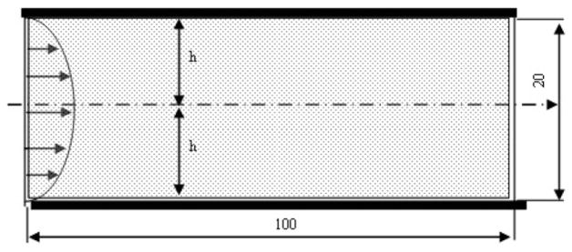
A 2D Poiseuille fluid flow between two parallel plates (dimensions in μm).

First, we obtain the FE solution with the velocity–pressure nodal variables in accordance with Eq. (46). We then model the flow using the DPD method for the whole domain to find the material constants of the DPD model by matching the velocity field derived from the DPD close to the analytical result. Finally, we implement the multiscale approach by coupling the DPD model and FE model.

The Reynolds number and viscosity are set to be Re = 10 and μ = 1.0 g/μms, respectively (viscosity corresponds to the constitutive law in Eq. (45)). The pressure drop, which is ∂p/∂x = 0.01 g/s²μm², is used to set the pressure boundary conditions in our FE model. It is assumed that the initial velocities are equal to zero. The FE solution calculated by using 9-node elements with pressures at the corner nodes [61,67] agrees with the analytical solution.

In the DPD model, the velocity of each DPD particle was prescribed at the entrance of the channel to match the inlet velocity condition with a parabolic profile of the analytical solution. The periodic boundary conditions were imposed for the inlet and outlet boundaries (e.g. [19,20]). The bounce-back method is used for the no-slip rigid wall boundary conditions [54]. A good agreement with the analytical solution was reached (Fig. 4) using a = 25, σ = 3, and γ = 4.5 (see Eqs. (39)–(41)). A time step used for the DPD simulation was Δt_DPD = 0.001, which corresponds to Δt_FE = 0.1 s for the macroscale FE model [54,55].

Fig. 4.

Analytical, DPD and FE solutions for velocity; 2D steady Poiseuille flow. Coordinate Y is normalized with respect to the channel width 2h = 20 [μm].

Next, we solve the same problem using a multiscale model. The finite element mesh is the same as before (10 elements in the lateral and 50 elements in the axial directions) and a DPD domain is placed in the middle of the channel, covering 6 × 6 finite elements, shown in Fig. 5. As the DPD domain is located symmetrically around the axis of symmetry, the velocity profile is symmetric laterally within the domain and an interaction with the FE solution is also symmetric. We used 2500 DPD particles for the box.

Fig. 5.

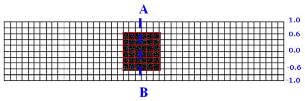
Finite element mesh with a DPD domain (box). The box is symmetrically positioned with respect to the axis of symmetry. The middle plane of the box is denoted as cross-section plane AB. Vertical coordinate is normalized.

Two types of boundary conditions are implemented for the DPD box:

1. Given velocities at the top and bottom lines parallel to flow; and

2. Periodic boundary conditions and given velocities at the entering and outlet boundaries.

We implemented the Lees–Edwards [52–54] method for the boundary conditions (a). According to this method, a particle crossing the upper boundary of the DPD domain at the end of a DPD time step Δt_DPD is re-introduced at the lower boundary with its x_u-coordinate shifted by −(v̄_x)_u × Δt_DPD and the x-velocity is decreased by (v̄_x)_u. Here (v̄_x)_u is the velocity obtained from the FE model. Further, a particle crossing the lower boundary, at a coordinate x_l and having the velocity (v̄_x)_l is re-introduced at the upper boundary of the box at x-coordinate shifted by (v̄_x)_l × Δt_DPD and the x-velocity is increased by (v̄_x)_l.

Regarding the boundary conditions (b), we used the usual periodic boundary conditions [19,20]: if a particle lives the box at the outlet within time step Δt_DPD, a particle is introduced at the same y-coordinate at the inlet boundary, with the boundary velocity obtained from the FE solution.

Temporal evolution of the velocity profile at the middle of the DPD domain simulated by the newly developed FE– DPD multiscale bridging method is compared to the FE (analytical) solution in Fig. 6. The results demonstrate that the multiscale solutions agree very well with the analytical solutions.

Fig. 6.

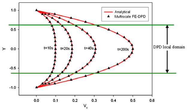
The time evolution of velocity profiles in Poiseuille flow. FE and multiscale FE-DPD solutions at AB plane cross-section (middle position of the left DPD box); Y coordinate normalized.

Fig. 7a shows the ultimate velocity profile over the DPD domain (A–B cross-section). The results are obtained using two different bin divisions for velocity averaging. In the first one, shown by large circles, the averaging goes over the bins obtained by 20 divisions of the DPD domain in the Y direction and no division in X direction (division 20 × 1). In the second division we have 20 divisions in both Y and X directions (division 20 × 20); the results are shown by small dots, where each dot corresponds to one bin. It can be noticed that bin division (20 × 1) gives results which are closer to the analytical solution. In Fig. 7b, the DPD solution is shown for several axial layers obtained by (20 × 20) bin division over the whole box. Note that the velocity profiles have some deviations from the analytical solution.

Fig. 7.

Velocity profile over DPD domain at AB cross-section for t = 200s (the DPD solutions correspond to averaging over the last 10,000 DPD time steps of the total 100,000 DPD time steps per one FE time step). (a) Analytical and multiscale solutions using velocity averaging over (20×1) and (20×20) DPD bins; (b) Analytical and multiscale solutions using velocity averaging over axial layers 1, 6 and 20 inside the DPD domain, with bin division (20×20).

Shear stress distribution along the AB line over the whole cross-section, calculated by the multiscale approach, was compared to the analytical solution (Fig. 8). The deviations of the DPD values of the shear stress come from the averaging over the DPD bins in Eq. (58).

Fig. 8.

Shear stress distribution along the AB line obtained by the multiscale approach vs. the FE (analytical) solution. The DPD shear stress values were obtained by averaging over (20×1) bins (Y coordinate normalized).

4.2. Example 2: Cavity flow

The driven cavity flow is chosen as a more complex problem (note that there are fluid zones with the stress singularity near the corners) which represents a recirculation flow with curve streamlines.

The flow in the cavity is induced by a horizontal motion of the upper wall with a constant velocity of V (Fig. 9). The Reynolds number, based on the size of the cavity and the velocity of the upper wall movement, was set to 30. A local DPD domain (a small square region in Fig. 9) was selected at the right upper corner of the cavity and the flow was solved both by the FE method alone and by the FE– DPD multiscale bridging method. In the DPD simulation, 900 mesoscale DPD particles were employed. The material parameters were set the same as in Example 1. The boundary conditions for the DPD simulation are as follows: at the no-slip rigid wall, the bounce-back condition was employed; at the moving wall it is assumed that particles have the prescribed velocity V = 1 μm/s; at the FE–DPD common boundaries, the velocities of particles are modeled as described in Section 3.4. The boundary conditions for the FE model consist of the prescribed velocity at the moving wall and zero velocity at the rigid walls. Also, the periodic boundary conditions are used for the entering (lower horizontal) and the outlet (left vertical) boundaries to keep number of particles within the DPD box constant. It is assumed that initial pressures and velocities in the whole domain are equal to zero.

Fig. 9.

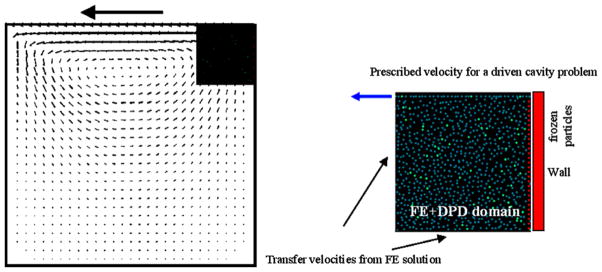
Driven cavity problem: multiscale FE-DPD model. Dimensions of the cavity are 30 × 30μm, and dimensions of the DPD box are 7.5×7.5μm. Velocities are prescribed (V=1μm/s) on the top boundary, from the right to the left. The flow domain is divided into the global FE domain and local FE-DPD domain. Boundary conditions for the DPD model are shown in the right figure.

The velocity components (v_x, v_y) along the vertical line, which goes through the middle of the local (FE + DPD) domain and extends through the global (FE) domain to the bottom of the cavity (see the insets in Fig. 10), are calculated both by the FE method alone and by the FE–DPD multiscale method. As can be seen from Fig. 10, the FE and multiscale solutions agree very well. Velocity vector profiles calculated by the FE method (Fig. 11 left) and by the FE– DPD multiscale method (Fig. 11 right) are also compared with good agreement. Finally, it is noted that the pressure has practically no effect on the solutions and that flow is governed by shear stresses.

Fig. 10.

Velocity profiles along the verticle middle-line (shown by vertical line in the insets) passing through the local (FE-DPD) and global (FE) domains. The final time, t=10 sec, is reached after total 2,000,000 DPD time steps (and 100 FE time steps). (a) Velocity component v_x; (b) Velocity component v_y.

Fig. 11.

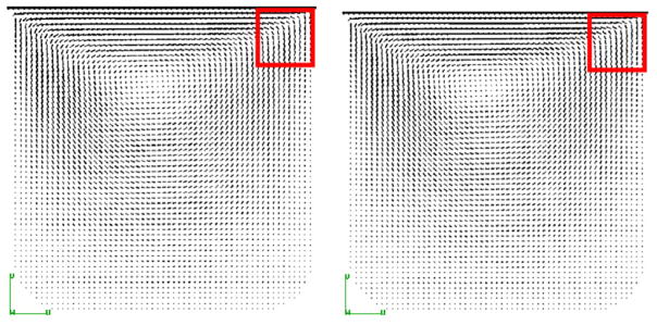
Velocity vector field for the FE method (left) and multiscale method (right).

5. Conclusions

The proposed mesoscopic bridging scale (MBS) method for fluids provides the coupling between mesoscale discrete particle models and continuum-based finite element models. It is an extension of the bridging scale method for coupling molecular dynamics and finite element models.

This multiscale approach can be applied to modeling a dilute mixture flow where in small local regions a detailed analysis of particle motions is desirable, as in case of blood flow in a large artery with platelet aggregation and adhesion to the vessel wall in a small domain of thrombosis development [42–45].

It can be seen from the presented examples that the proposed approach of coupling the mesoscopic DPD model and continuum FE model is applicable to incompressible fluid flow. Further, it is important to note that iterations on the DPD solution were performed until the equilibrium is reached, with the velocity boundary conditions imposed from FE solution for each FE time step. Also, we calculated the stresses by averaging over the last 10% of DPD time steps when the solution is close to the equilibrium state. And we found that the random character of the total interaction DPD forces does not cause noticeable noise outside the DPD domain. The noise effects are small for small and moderate Reynolds numbers (in our examples Re was around 30). Investigation of these effects will be the subject of another study.

References

- 1.Gerstein M, Levitt M. Simulating water and the molecules of life. Sci Am. 2005:24–29. doi: 10.1038/scientificamerican1198-100. (The Water of Life Special Issue) [DOI] [PubMed] [Google Scholar]
- 2.Flekkoy EG, Coveney PV. From molecular dynamics to dissipative particle dynamics. Phys Rev Lett. 1999;83:1775–1778. [Google Scholar]
- 3.Flekkoy EG, Coveney PV, De Fabritiis G. Foundations of dissipative particle dynamics. Phys Rev E. 2000;62:2140–2157. doi: 10.1103/physreve.62.2140. [DOI] [PubMed] [Google Scholar]
- 4.Serrano M, De Fabritiis G, Espanol P, Flekoy EG, Coveney PV. Mesoscopic dynamics of Voronoy fluid particles. J Phys A. 2002;35:1605–1625. [Google Scholar]
- 5.Monaghan JJ. Smoothed particle hydrodynamics. Annu Rev Astron Astrophys. 1992;30:543–574. [Google Scholar]
- 6.Hoogerbrugge PJ, Koelman JMVA. Simulating microscopic hydrodynamic phenomena with dissipative particle dynamics. Europhys Lett. 1992;19:155–160. [Google Scholar]
- 7.Espanol P. Hydrodynamics from dissipative particle dynamics. Phys Rev E. 1995;52(2):1734–1742. doi: 10.1103/physreve.52.1734. [DOI] [PubMed] [Google Scholar]
- 8.Espanol P, Warren P. Statistical mechanics of dissipative particle dynamics. Europhys Lett. 1995;30(4):191–196. [Google Scholar]
- 9.Espanol P, Serrano M, Zuniga I. Coarse-graining of a fluid and its relation with dissipative particle dynamics and smoothed particle dynamics. Int J Mod Phys C. 1997;8(4):899–908. [Google Scholar]
- 10.Espanol P. Dissipative particle dynamics with energy conservation. Europhys Lett. 1997;40(6):631–636. [Google Scholar]
- 11.Coveney PV, Espanol P. Dissipative particle dynamics for interacting multicomponent systems. J Phys A. 1997;30:779–784. [Google Scholar]
- 12.Espanol P. Fluid particle model. Phys Rev E. 1998;57:2930–2948. [Google Scholar]
- 13.Espanol P, Serrano M. Dynamics regimes in the dissipative particle dynamics model. Phys Rev E. 1999;59(6):6340–6347. doi: 10.1103/physreve.59.6340. [DOI] [PubMed] [Google Scholar]
- 14.Ripoll M, Ernst MH, Espanol P. Large scale mesoscopic hydrodynamics for dissipative particle dynamics. J Chem Phys. 2001;115(15):7271–7284. [Google Scholar]
- 15.Espanol P, Vazquez F. Coarse graining from coarse grained descriptions. Philos Trans Roy Soc London Ser A. 2002;A360:1–12. doi: 10.1098/rsta.2001.0935. [DOI] [PubMed] [Google Scholar]
- 16.Espanol P, Revenga M. Smoothed dissipative particle dynamics model. Phys Rev E. 2003;67:026705-1–026705-12. doi: 10.1103/PhysRevE.67.026705. [DOI] [PubMed] [Google Scholar]
- 17.Avalos JB, Mackie AD. Dissipative particle dynamics with energy conservation. Europhys Lett. 1997;40(2):141–146. [Google Scholar]
- 18.Marsh C. PhD thesis. U. Oxford; 1998. Theoretical aspects of dissipative particle dynamics. [Google Scholar]
- 19.Besold G, Vattulainen I, Karttunen M, Polson JM. Toward better integrators for dissipative particle simulations. Phys Rev E. 2000;62(6):R7611–R7614. doi: 10.1103/physreve.62.r7611. [DOI] [PubMed] [Google Scholar]
- 20.Novik KE, Coveney PV. Using dissipative particle dynamics to model binary immiscible fluids. Int J Mod Phys C. 1997;8(4):909–918. doi: 10.1103/physreve.54.5134. [DOI] [PubMed] [Google Scholar]
- 21.Groot RD, Warren PB. Dissipative particle dynamics: Bridging the gap between atomistic and mesoscopic simulation. J Chem Phys. 1997;107(11):4423–4435. [Google Scholar]
- 22.Boryczko K, Dzwinel W, Yuen DA. Dynamic clustering of red blood cells in capillary vessels. J Mol Model. 2003;9:16–33. doi: 10.1007/s00894-002-0105-x. [DOI] [PubMed] [Google Scholar]
- 23.Dzwinel W, Boryczko K, Yuen DA. A discrete-particle model of blood dynamics in capillary vessels. J Colloid Interf Sci. 2003;258:163–173. doi: 10.1016/s0021-9797(02)00075-9. [DOI] [PubMed] [Google Scholar]
- 24.Visser DC, Hoefsloot HCJ, Iedema PD. Modelling multi-viscosity systems with dissipative particle dynamics. J Comput Phys. 2006;214(2):491–504. [Google Scholar]
- 25.Curtin WA, Miller RE. Atomistic/continuum coupling in computational material science. Model Simul Mater Sci Engrg. 2003;11:R33–R68. [Google Scholar]
- 26.Liu WK, Karpov EG, Zhang S, Park HS. An introduction to computational nanomechanics and materials. Comput Methods Appl Mech Engrg. 2004;193:1529–1578. [Google Scholar]
- 27.Liu WK, Qian D, Horstemeyer MF. Preface. Comput Methods Appl Mech Engrg. 2004;193:iii–iv. Special Issue. [Google Scholar]
- 28.Nielsen SO, Lopez CF, Srinivas G, Klein ML. Coarse grain models and computer simulation of soft materials. J Phys: Condens Matter. 2004;16:R481–R512. [Google Scholar]
- 29.Wagner GJ, Liu WK. Coupling of atomistic and continuum simulations using a bridging scale decomposition. J Comput Phys. 2003;190:249–274. [Google Scholar]
- 30.Tang S, Hou TH, Liu WK. A mathematical framework of the bridging scale method. Int J Num Methods Engrg. 2006;65:1688–1713. [Google Scholar]
- 31.Qian D, Wagner GJ, Liu WK. A multiscale projection method for the analysis of carbon nanotubes. Comput Methods Appl Mech Engrg. 2004;193:1603–1632. [Google Scholar]
- 32.Kadowaki H, Liu WK. Bridging multi-scale method for localized problems. Comput Methods Appl Mech Engrg. 2004;193:3267–3302. [Google Scholar]
- 33.Park HS, Karpov EG, Liu WK. A temperature equation for coupled atomistic/continuum simulations. Comput Methods Appl Mech Engrg. 2004;193:1713–1732. [Google Scholar]
- 34.Park HS, Karpov EG, Klein PA, Liu WK. Three-dimensional bridging scale analysis of dynamic fracture. J Comput Phys. 2005;207:588–609. [Google Scholar]
- 35.Park HS, Karpov EG, Liu WK, Klein PA. The bridging scale for two-dimensional atomistic/continuum coupling. Philos Mag. 2005;85(1):79–113. [Google Scholar]
- 36.Zhang L, Gerstenberger A, Wang X, Liu WK. Immersed finite element method. Comput Methods Appl Mech Engrg. 2004;193:2015–2067. [Google Scholar]
- 37.Liu WK, Liu Y, Farrell D, Zhang L, Wang XS, Fukui Y, Patankar N, Zhang Y, Bajaj C, Lee J, Hong J, Chen X, Hsua H. Immersed finite element method and its applications to biological systems. Comput Methods Appl Mech Engrg. 2006;195:1722–1749. doi: 10.1016/j.cma.2005.05.049. [DOI] [PMC free article] [PubMed] [Google Scholar]
- 38.Karpov EG, Wagner GJ, Liu WK. A Green’s function approach to deriving non-reflecting boundary conditions in molecular dynamics simulations. Int J Num Methods Engrg. 2005;62:1250–1262. [Google Scholar]
- 39.Filipovic N, Kojic M, Tsuda A. Modeling of microcirculation and thrombosis by dissipative particle dynamics (DPD), (Abstract). Fifth World Congress of Biomechanics; Munich. 2006. [Google Scholar]
- 40.Filipovic N, Ravnic D, Kojic M, Mentzer SJ, Haber S, Tsuda A. Interactions of blood cell constituents: Experimental investigation and computational modeling by discrete particle dynamics algorithm. Microvasc Res. doi: 10.1016/j.mvr.2007.09.007. in press. [DOI] [PubMed] [Google Scholar]
- 41.Filipovic N, Kojic M, Tsuda A. Modeling of thrombosis using dissipative particle dynamics, invited paper. Phil Trans A. doi: 10.1098/rsta.2008.0097. in preparation. [DOI] [PMC free article] [PubMed] [Google Scholar]
- 42.Kojic M, Filipovic N, Tsuda A. In: Kojic M, Papadrakakis M, editors. A multiscale method for bridging dissipative particle dynamics and Navier–Stokes finite element equations for incompressible fluid and its application in biomechanics; Proceedings of the First South-East European Conference on Computational Mechanics; Kragujevac, Serbia. 2006. [Google Scholar]
- 43.Kojic M, Filipovic N, Tsuda A. Multiscale modeling of blood flow: coupling dissipative particle method and finite element method, (Abstract). Fifth World Congress of Biomechanics; Munich. 2006. [Google Scholar]
- 44.Kojic M, Filipovic N, Stojanovic B, Kojic N. Examples and Software. J. Wiley & Sons; Computer Modeling in Bioengineering – Theoretical Background. in press. [Google Scholar]
- 45.Kojic M, Filipovic N, Tsuda A. Multiscale modeling of platelet-mediated thrombosis in large blood vessels. in preparation. [Google Scholar]
- 46.de With G. Structure Deformation and Integrity of Materials. Wiley VCH; 2005. [Google Scholar]
- 47.Ren W, WE Heterogeneous multiscale method for the modeling of complex fluids and micro-fluidics. J Comput Phys. 2005;204:1–26. [Google Scholar]
- 48.Filippova O, Succi S, Mazzocco F, Arrighetti C, Bella G, Hanel D. Multiscale lattice Boltzmann schemes with turbulence modeling. J Comput Phys. 2001;170:812–829. [Google Scholar]
- 49.Bathe KJ. Finite Element Procedures. Prentice-Hall; Englewood Cliffs, NJ: 1996. [Google Scholar]
- 50.Revenga M, Zuniga I, Espanol P, Pagonabarraga I. Boundary models in DPD. Int J Mod Phys C. 1998;9:1319–1331. [Google Scholar]
- 51.Willemsen SM, Hoefsloot HCJ, Iedema PD. No-slip boundary condition in dissipative particle dynamics. Int J Mod Phys C. 2000;11(5):881–890. [Google Scholar]
- 52.Hong DD, Thien NP, Fan X. An implementation of no-slip boundary conditions in DPD. Comput Mech. 2004;35:24–29. [Google Scholar]
- 53.Pivkin I, Karniadakis GE. A new method to impose no-slip boundary conditions in dissipative particle dynamics. J Comput Phys. 2005;207:114–128. doi: 10.1016/j.jcp.2011.02.003. [DOI] [PMC free article] [PubMed] [Google Scholar]
- 54.Haber S, Filipovic N, Kojic M, Tsuda A. Dissipative particle dynamics simulation of flow generated by two rotating concentric cylinders. Phys Rev E. 2006;74:1–8. doi: 10.1103/PhysRevE.74.046701. [DOI] [PubMed] [Google Scholar]
- 55.Filipovic N, Kojic M, Haber S, Tsuda A. Computational validation of dissipative particle dynamics simulation on a benchmark example. submitted for publication. [Google Scholar]
- 56.Cai W, de Koning M, Bulatov VV, Yip S. Minimizing boundary reflections in coupled-domain simulations. Phys Rev Lett. 2000;85(15):3213–3216. doi: 10.1103/PhysRevLett.85.3213. [DOI] [PubMed] [Google Scholar]
- 57.Wagner GJ, Karpov EG, Liu WK. Molecular dynamics boundary conditions for regular crystal lattices. Comput Methods Appl Mech Engrg. 2004;193:1579–1601. [Google Scholar]
- 58.Huebner KH. The Finite Element Method for Engineers. J. Wiley & Sons; Chichester, UK: 1975. [Google Scholar]
- 59.Kojic M, Slavkovic R, Zivkovic M, Grujovic N. Faculty of Mech Engrg. Univ. Kragujevac; Kragujevac, Serbia: 1998. The Finite Element Method I – Linear Analysis (in Serbian) [Google Scholar]
- 60.Kojic M, Filipovic N, Slavkovic R, Zivkovic M, Grujovic N. PAK-F, Finite Element Program for Fluid Flow and Mass and Heat Transfer. Univ. Kragujevac; Kragujevac, Serbia: 1998. [Google Scholar]
- 61.Filipovic N, Mijailovic S, Tsuda A, Kojic M. An implicit algorithm within the arbitrary Lagrangian–Eurlerian formulation for solving incompressible fluid flow with large boundary motions. Comput Methods Appl Mech Engrg. 2006;195:6347–6361. [Google Scholar]
- 62.Kojic M, Bathe KJ. Inelastic Analysis of Solids and Structures. Springer; Berlin, Heidelberg: 2005. [Google Scholar]
- 63.Fan X, Phan-Thien N, Yong NT, Wu X, Xu D. Microchannel flow of a macromolecular suspension. Phys Fluids. 2003;15:11–21. [Google Scholar]
- 64.Kojic M, Filipovic N, Tsuda A. Multiscale acinar airflow modeling coupling microscale dissipative particle dynamics (DPD) method and macroscale finite element (FE) method, (Abstract). BMES Conference; Chicago. 2006. [Google Scholar]
- 65.Vattulainen I, Karttunen M, Besold G, Polson JM. Integration schemes for dissipative particle dynamics simulations: From softly interacting systems towards hybrid models. J Chem Phys. 2002;116(10):3967–3979. [Google Scholar]
- 66.Jakobsen AF, Mouritsen OG. Artifacts in dynamical simulations of coarse-grained model lipid bilayers. J Chem Phys. 2005;122:204901–204911. doi: 10.1063/1.1900725. [DOI] [PubMed] [Google Scholar]
- 67.Filipovic N, Kojic M. Computer simulations of blood flow with mass transport through the carotid artery bifurcation. Theoret Appl Mech (Serbian) 2004;31(1):1–33. [Google Scholar]