

Abstract
We introduce a new hybrid molecular orbital/density-functional modified divide-and-conquer (mDC) approach that allows the linear-scaling calculation of very large quantum systems. The method provides a powerful framework from which linear-scaling force fields for molecular simulations can be developed. The method is variational in the energy, and has simple, analytic gradients and essentially no break-even point with respect to the corresponding full electronic structure calculation. Furthermore, the new approach allows intermolecular forces to be properly balanced such that non-bonded interactions can be treated, in some cases, to much higher accuracy than the full calculation. The approach is illustrated using the second-order self-consistent charge density-functional tight-binding model (DFTB2). Using this model as a base Hamiltonian, the new mDC approach is applied to a series of water systems, where results show that geometries and interaction energies between water molecules are greatly improved relative to full DFTB2. In order to achieve substantial improvement in the accuracy of intermolecular binding energies and hydrogen bonded cluster geometries, it was necessary to extend the DFTB2 model to higher-order atom-centered multipoles for the second-order self-consistent intermolecular electrostatic term. Using generalized, linear-scaling electrostatic methods, timings demonstrate that the method is able to calculate a water system of 3000 atoms in less than half of a second, and systems of up to one million atoms in only a few minutes using a conventional desktop workstation.
1 Introduction
There is great interest in the scientific community to develop molecular simulation force fields that are able to explicitly treat electronic degrees of freedom in order to model chemical and biochemical phenomena that are inherently related to electronic structure. Example applications include simulations of reactive chemical events such as catalysis,1 photochemistry and electron transfer processes,2–4 as well as the calculation of spectroscopic observables to aid in the interpretation of experiments.5,6 Toward that end, quantum chemical methods are required that are fast, accurate, and can scale to the large system sizes and long time scales required by the applications. The scaling requirement has been a long-standing arena of active research effort in the development of so-called “linear-scaling” - O(N) or O(N log N) - electronic structure methods, for which much success has been achieved.7–13
Nonetheless, there remain challenges that prevent these established linear-scaling electronic structure methods from being used as practical tools, and having broad impact, in truly large-scale molecular dynamics simulations. Firstly, despite having favorable scaling properties, the computational cost of conventional linear-scaling methods is typically still prohibitive for long-time simulations of large systems, although some applications are beginning to emerge.14–21 This is related to the fact that these methods typically have break-even points of a few hundreds of atoms, only after which do the methods have any computational advantage relative to their full nonlinear-scaling counterparts.22 Secondly, for condensed phase simulations, methods need to accurately treat both strong intramolecular (i.e., bonding) interactions and subtle, typically weak intermolecular (i.e., nonbonding) interactions. The latter needs to be delicately balanced such that bulk properties, binding affinities, and solvation free energies are treated accurately and consistently. This balance remains a challenge for modern density-functional methods, even without consideration of extension to linear-scaling.23 Thirdly, to make these methods practical for molecular dynamics simulations, rigorous analytic gradients are needed that require only relatively minor overhead relative to the calculation of the energy itself.21,24
In this work, we introduce a new modified divide-and-conquer (mDC) approach that allows the linear-scaling calculation of very large quantum systems, including analytic gradients, with essentially no break-even point. The extended atomic orbital (AO) buffer space used in traditional divide-and-conquer (DC) is replaced by a density-overlap intermolecular interaction model25 that is treated self-consistently and can be tuned for high accuracy. The approach is illustrated using the second-order self-consistent field density-functional tight-binding (SCC-DFTB or DFTB2) model.26 Using DFTB2 as a base Hamiltonian, the new mDC approach is applied to a series of water systems, where results show that geometries and interaction energies between water molecules are greatly improved relative to full DFTB2, whereas timings demonstrate that the method may be practical for large-scale molecular dynamics (MD) simulations. The method is demonstrated to be highly scalable, and able to calculate systems of up to one million atoms in only a few minutes using a conventional desktop workstation.
2 Methods
2.1 Essential Background
Next generation MO-based force fields are founded upon linear-scaling electronic structure theory to reduce the scaling bottlenecks associated with the underlying ab initio model; however, unlike traditional linear-scaling electronic structure methods, the Hamiltonian form is modified with empirical potentials and parameters to increase performance and make the resulting method more accurate. The concept of using electronic structure theory explicitly as a “next generation quantum force field” was introduced by Gao,27 who demonstrated its accuracy for liquid simulations28 and explored its feasibility for use in treating biological molecules.29 There are other approaches, such as SIBFA30,31 and GEM30,32–34 that may also be considered quantum force fields, but do not explicitly use MOs. These density-based models approximate the exchange-repulsion between fragments using a density-overlap model.35 The present work makes explicit use of MOs, like those models described by Gao, and treats the inter-region coupling with a density-overlap model that is influenced by the SIBFA and GEM methods.
Consider the case of a quantum chemical method based on a single determinant wave function that is variationally optimized to minimize the total electronic energy (e.g., Hartree-Fock, and most modern density-functional or semiempirical quantum methods fit this category.) The two most expensive mathematical operations performed during the self consistent field (SCF) procedure on large systems are the construction of the Fock matrix elements and its diagonalization. Several methods have been introduced for computing the Fock matrix with O(N log N) effort.36–39 The dominant part of this effort is spent performing the electrostatic interactions39–46 because of their significance even between well-separated atoms. Most methods for overcoming the O(N3)-scaling of the Fock matrix diagonalization are exploitations of the sparse matrices that arise due to the negligible overlap between well-separated atoms. As a simple illustration of how this property reduces the scaling of the diagonalization, consider a system composed of two regions A and B. When the two regions are sufficiently separated, their inter-region overlap is negligibly small and the inter-region Fock matrix elements necessarily vanish. In this case, the wavefunction of the system can then be accurately approximated by a Hartree product of antisymmetrized determinants of molecular fragments.27 The eigenvalues E and eigenvectors C of the system then satisfy
| (1) |
where FA · CA = SA · CA · EA, SA is the intra-region overlap, and region B diagonalizes analogously. In other words, diagonalization of the full system is equivalent to the diagonalization of the smaller systems. The scaling thus reduces to O(NK3), where K is the size of a single region. This does not imply that the systems are isolated, however. FA and FB are the nonzero diagonal blocks of the Fock matrix, and these include the potentials arising from both regions, which is longer-ranged than the inter-region overlap.
When the two regions above are not well-separated, they remain coupled by inter-region overlap, and one must concoct a scheme to account for it. For example, the method used in the X-Pol model is to replace the explicit coupling with empirical Lennard-Jones or Buckingham potentials29,47–53 or through perturbative corrections.54,55 The Fragment Molecular Orbital (FMO) method56–62 computes the variational energy of decoupled regions and then reintroduces the inter-region coupling via many-body expansion corrections solved in the presence of the fixed electrostatic potential of the other regions as determined from the decoupled calculation. This makes the FMO total energy non-variational and thus complicates the implementation of its analytic gradients.57 Other fragment-based methods exist that treat the coupling with many-body perturbative expansions.63–65 The divide-and-conquer (DC) scheme16,17,19,22,24,66–82 accounts for the coupling by explicitly extending the AO-space of the region to include its near-neighbor regions, called its “buffer.” The resulting molecular orbitals (MOs) extend beyond the region and into its buffer. Special care must then be placed to partition the resulting electron density to avoid its double counting when the region is treated as its neighbor’s buffer. The fragment density functional method is similar to DC: each region is surrounded by a buffer and the system outside of the buffer is treated by empirical point charges.51,83
Rigorous analytic gradients of buffered DC require the solution of the coupled perturbed Hartree-Fock/Kohn-Sham equations of the entire system.24 The solution of these equations is difficult to achieve in a linear-scaling fashion. Fortunately, the approximate analytic formulas for the buffered DC method are sufficient so as long as the buffer is large (≈ 4 to 5 Å) but produce unacceptably large errors when the size of the buffer is small. The mDC method described in the present work circumvents the need to solve the coupled-perturbed equations by replacing the explicit buffer space with a density-overlap intermolecular interaction model. Without an explicit buffer, the gradient expressions for each region are no more difficult than those encountered in traditional single-determinant methods.
2.2 The mDC Energy
In the context of mDC, we consider a “region” to be a fragment of the system whose AOs are chosen to be completely localized on that fragment. In this manner, the Fock matrix for a fragment can be diagonalized to produce it’s own set of local MOs. The mDC total energy is then described as the sum of the energy of each region EA and the inter-region interactions.
| (2) |
where A and B index regions; a and b index atoms; α and β denote electron spin; R is the full set of atomic coordinates; q is the full set atomic multipole moments; and qa and qA are the multipole moments of atom a and the collection of atomic multipole moments in region A, respectively.
| (3) |
is the single-particle spin-resolved density matrix of region A; is the spin-resolved occupation number of orbital k in region A; is the ith MO coefficient of orbital k in region A, which satisfy
| (4) |
The multipole moments of atom a are
| (5) |
where Za is the core nuclear charge of atom a; Clm(r) is a real regular solid harmonic; and ρa(r) is the partitioned atomic density of atom a, which shall be discussed in more detail later.
| (6) |
is the Coulomb electrostatic energy between point-multipoles, i.e.,
| (7) |
where
| (8) |
is a point-multipole function; Clm(∇a) is a spherical tensor gradient operator 84 acting on the coordinates of atom a; and δ (r) is a Dirac-delta function.
EA(Pα,A,Pβ,A,qA; RA) is the quantum energy of region A, which for this work is the DFTB2 model described in numerous articles.26,85–88 In brief,
| (9) |
where PA = Pα,A +Pβ,A is the total density matrix; H is the tight-binding matrix constructed from two-center splines and one-center parameters; Erep(Rab) is a pairwise repulsive potential stored on splines; and
| (10) |
is the Coulomb interaction between the auxiliary Slater monopole representation of the response density, i.e.,
| (11) |
In this work Einter,ab(qa, qb; Rab) is chosen to be the OPNQ van der Waals (vdW) model described in Ref. 25, where
| (12) |
The exchange energy
| (13) |
is the overlap of Slater monopoles with a charge-dependent exponent
| (14) |
where sa, ςa(0), and ha are parameters. The dispersion energy is
| (15) |
where bab ≡ bab(qa, qb, Rab)
| (16) |
is the Tang and Toennies (TT) damping exponent;
| (17) |
is a charge-dependent dispersion coefficient;
| (18) |
| (19) |
is the effective number of valence electrons;
| (20) |
is the number of valence electrons and Nval,a(0) is the number of valence electrons in the neutral atom;
| (21) |
is the charge-dependent dipole polarizability, where αa(0) and fa are treated as parameters and the Neff,a(0) parameters are taken from Ref. 89. The TT damping function is
| (22) |
2.3 The mDC Fock Matrix and SCF Procedure
The spin-resolved Fock matrix of region A is
| (23) |
where p is a vector of “multipolar potentials”, i.e.,
| (24) |
The dependence of the inter-region interactions on the density matrices occur entirely through the atomic multipole moments, and therefore the Fock matrix need only be corrected by reverse-mapping the multipolar potentials. The mapping of the density matrices to the multipole moments is a choice. In this work we suppose
| (25) |
where χi(r) = χi(r)Ylimi (Ω) is an atomic orbital basis function and Ylm(Ω) is a real spherical harmonic. Furthermore, we limit the multipole expansion of the two-center densities to monopole so that the resulting multipole expansions consist of Mulliken charges and the high-order moments of the one-center densities. Inserting Eq. (25) into Eq. (5) with this constraint produces
| (26) |
and
| (27) |
for la > 0, where
| (28) |
are tabulated constants and
| (29) |
is dependent on the radial behavior of the AOs. In the present work there are only two cases to consider:
| (30) |
and
| (31) |
where O2s(r) and O2p(r) are the radial-components of the 2s and 2 p AOs of oxygen. These integrals are readily computed from quadrature using the AOs resulting from atomic calculations; however, we treat the value of these integrals as parameters to tune the accuracy of the intermolecular interactions, which leads to significant improvement.
The derivatives required for mapping the multipolar potentials into the Fock matrix are then
| (32) |
and
| (33) |
for la > 0 and i j ∈ a.
The Fock matrix is used within the SCF procedure to generate new guess orbitals as described in Figure 1.
Figure 1.
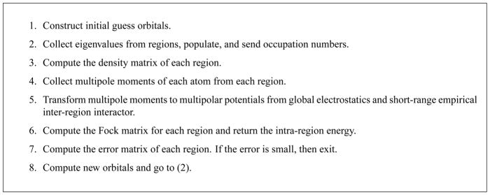
The mDC SCF procedure.
The above mapping of the density matrix to the auxiliary basis representation is simple in the present demonstration. Nonetheless, more sophisticated and rigorous procedures have been described in our previous works,90,91 which also mapped the two-center density components to high-order Gaussian multipoles.92 These methods may provide tools that extend the current work, and enable the development of other linear-scaling quantum methods to be developed using higher-level quantum base models with less parameters.
2.4 The mDC Gradients
As described above, the total mDC energy is variationally minimized, and thus the analytic gradient formulas are no more complicated than those encountered in traditional single-determinant methods. Suppose atom c is in region A, then its gradient in the X-direction is
| (34) |
where
| (35) |
2.5 Computational Details
We examine the binding energies and geometries of small water clusters and measure wall-clock timings of large “water spheres”, like those used in stochastic boundary simulations. The spheres were constructed from an equilibrated 216 TIP3P water box (18.86 Å cube) which was replicated periodically and cut to the desired size. The water cluster reference binding energies result from unconstrained geometry optimization with MP2(FULL)/6-311++G** (referred to as “MP2” henceforth) using the Gaussian 09 (revision A.02) software package.93 These energies are adiabatic MP2 electronic energies; i.e., vibrational corrections are not applied. The MP2 water dimer interaction energy is −6.13 kcal/mol, which is in reasonable agreement with the experimental estimate94 of −5.4±0.7 kcal/mol; however, counterpoise-corrected CCSD(T) in the complete basis set limit predicts95 an interaction energy of −5.0 kcal/mol. One might therefore consider the MP2 value to be too attractive. We’ve chosen to parametrize the model against the MP2 data to compensate for DFTB2’s under-prediction of the water polarizability. For comparison, the TIP3P water model produces a dimer interaction energy of −6.59 kcal/mol while still being considered useful for condensed phase simulations. The tables and figures of this manuscript will compare results to MP2, MP2+CP, and 〈MP2〉, where MP2+CP is the counterpoise corrected MP2(FULL)/6-311++G** energies and 〈MP2〉 is the average between the MP2 and MP2+CP energies. MP2+CP and 〈MP2〉 produce dimer interaction energies of −4.47 and −5.30 kcal/mol, respectively. Based on the water dimer interaction energy of −5.0 kcal/mol, the MP2 results are too attractive and the MP2+CP results are not attractive enough. We demonstrate that the parametrized model agrees more closely with the reference results than does standard DFTB2 irregardless of which of these ab initio results is used as a reference.
To determine the parameters in the mDC model, we constructed a water dimer MP2 binding energy curve as a function of oxygen separation (see Figure 2) and adjusted the parameter so that the long-range tail was reproduced. The parameter was adjusted so that the “wag angle” (angle b in Figure 3 and Table 1) of the water dimer was reproduced. The remaining vdW parameters were adjusted to reproduce the water cluster relative energies (Table 3 and Table 4) and water dimer binding energy curve. For comparison purposes, we also introduce a model called mDC(q), which is constructed in the same way as mDC; however, the and parameters are zero so that the inter-region interactions involve Mulliken charges only.
Figure 2.

Water dimer PESs.
Figure 3.
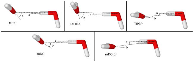
Comparison of water dimer geometries.
Table 1.
Water dimer geometry and interaction energies
| Method | ΔE kcal/mol | RO–O Å | a | b |
|---|---|---|---|---|
|
| ||||
| degrees | ||||
| MP2 | −6.13 | 2.91 | 2.1 | 44.1 |
| MP2+CP | −4.47 | ··· | ··· | ··· |
| 〈MP2〉 | −5.30 | ··· | ··· | ··· |
| DFTB2 | −3.32 | 2.86 | 3.6 | 65.5 |
| mDC | −5.83 | 2.91 | 0.7 | 43.0 |
| mDC(q) | −2.62 | 2.91 | 7.1 | 14.3 |
| TIP3P | −6.59 | 2.77 | 4.3 | 21.0 |
Table 3.
Cluster binding energies for each method and mDC and DFTB2 root mean square values. All energies are kcal mol−1. Coordinate rms values (a.u.) are relative to the structure before geometry optimization, which are the DFTB2 isolated waters superimposed onto the optimized MP2 cluster geometry.
| Cluster | ΔE
|
rms
|
|||||
|---|---|---|---|---|---|---|---|
| MP2 | MP2+CP | 〈MP2〉 | mDC | DFTB2 | mDC | DFTB2 | |
| (H2O)2 | −6.13 | −4.47 | −5.30 | −5.83 | −3.32 | 0.03 | 0.19 |
| (H2O)3 uud | −17.92 | −13.88 | −15.90 | −15.11 | −9.62 | 0.20 | 0.31 |
| (H2O)3 uuu | −17.11 | −13.28 | −15.19 | −13.93 | −8.79 | 0.26 | 0.31 |
| (H2O)4 1_udud | −31.57 | −24.35 | −27.96 | −26.87 | −17.69 | 0.17 | 0.16 |
| (H2O)4 2_uudd | −30.53 | −23.40 | −26.97 | −25.75 | −16.94 | 0.18 | 0.22 |
| (H2O)4 6 | −24.15 | −18.34 | −21.25 | −20.81 | −13.07 | 0.40 | 0.75 |
| (H2O)4 7 | −24.07 | −18.27 | −21.17 | −20.60 | −13.53 | 0.48 | 2.03 |
| (H2O)4 8 | −18.99 | −13.50 | −16.25 | −18.37 | −10.25 | 0.17 | 0.11 |
| (H2O)5 Puckered_ring | −41.93 | −32.10 | −37.01 | −35.53 | −23.03 | 0.20 | 0.39 |
| (H2O)5 Envelope | −40.35 | −30.78 | −35.57 | −34.10 | −23.03 | 1.08 | 1.23 |
| (H2O)5 Tetramer_trimer | −40.15 | −30.87 | −35.51 | −34.16 | −22.37 | 0.23 | 0.32 |
| (H2O)5 Tricycle | −39.08 | −29.94 | −34.51 | −32.61 | −22.47 | 0.34 | 0.96 |
| (H2O)5 Tetramer_1 | −37.55 | −28.58 | −33.06 | −32.03 | −20.75 | 0.20 | 0.53 |
| (H2O)5 Double_trimer | −35.66 | −27.38 | −31.52 | −29.91 | −19.21 | 0.37 | 0.66 |
| (H2O)5 Cage | −33.05 | −24.63 | −28.84 | −29.34 | −18.87 | 0.18 | 0.21 |
| (H2O)6 Prism | −52.18 | −39.92 | −46.05 | −44.54 | −29.60 | 0.20 | 0.21 |
| (H2O)6 Chair | −52.02 | −40.01 | −46.01 | −44.38 | −28.23 | 0.26 | 0.21 |
| (H2O)6 Book | −51.75 | −39.64 | −45.69 | −43.79 | −28.88 | 0.26 | 0.31 |
| (H2O)6 Open_bag | −51.47 | −39.22 | −45.34 | −43.31 | −28.67 | 0.28 | 0.37 |
| (H2O)6 Prism_book | −51.09 | −38.66 | −44.87 | −42.96 | −28.53 | 0.42 | 0.54 |
| (H2O)6 Boat | −50.83 | −38.86 | −44.85 | −43.22 | −27.59 | 0.42 | 0.23 |
| (H2O)6 Twisted_boat | −50.80 | −38.91 | −44.85 | −43.14 | −27.73 | 0.41 | 1.80 |
| (H2O)6 Intermediate_bag | −50.73 | −38.71 | −44.72 | −42.93 | −27.88 | 1.35 | 1.33 |
| (H2O)6 Double_tetramer | −50.70 | −39.26 | −44.98 | −42.45 | −28.10 | 0.47 | 0.42 |
| (H2O)6 Pentamer_down_1 | −50.68 | −38.85 | −44.77 | −43.07 | −27.87 | 0.32 | 0.54 |
| (H2O)6 Pentamer_planar_1 | −50.47 | −38.66 | −44.57 | −43.24 | −27.80 | 0.50 | 0.39 |
| (H2O)6 Cage | −50.31 | −38.61 | −44.46 | −42.60 | −28.52 | 0.28 | 0.45 |
| (H2O)6 Double_envelope | −48.83 | −37.59 | −43.21 | −41.84 | −27.35 | 0.37 | 0.41 |
| (H2O)6 Tetramer_trimer | −48.80 | −37.53 | −43.16 | −40.92 | −26.74 | 0.34 | 0.65 |
| (H2O)6 Tricycle_1a | −47.65 | −36.35 | −42.00 | −40.40 | −27.54 | 0.35 | 1.18 |
| (H2O)6 Closed_bag | −47.08 | −35.93 | −41.50 | −40.10 | −26.32 | 0.37 | 0.51 |
| (H2O)6 Tricycle_1b | −46.79 | −35.45 | −41.12 | −39.96 | −26.33 | 0.22 | 0.69 |
| (H2O)6 Triple_trimer | −43.01 | −33.13 | −38.07 | −36.10 | −27.67 | 0.46 | 2.88 |
Table 4.
Summary of mDC and DFTB2 cluster binding energy (ΔE) and cluster relative energies (ΔΔE) errors (kcal mol−1) relative to the MP2, MP2+CP, and 〈MP2〉 reference values. The coordinate root mean square statistics (a.u.) are relative to the structure before geometry optimization, which are the DFTB2 isolated waters superimposed onto the optimized MP2 cluster geometry.
| Ref. | Cluster | ΔE
|
ΔΔE
|
rms
|
||||
|---|---|---|---|---|---|---|---|---|
| mDC | DFTB2 | mDC | DFTB2 | mDC | DFTB2 | |||
| MP2 | (H2O)4 | mse | 3.38 | 11.57 | −1.65 | −2.90 | ··· | ··· |
| mue | 3.38 | 11.57 | 1.69 | 2.90 | 0.28 | 0.66 | ||
| max | 4.78 | 13.89 | −4.08 | −5.15 | 0.48 | 2.03 | ||
| (H2O)5 | mse | 5.73 | 16.86 | −0.78 | −2.38 | ··· | ··· | |
| mue | 5.73 | 16.86 | 0.80 | 2.38 | 0.37 | 0.61 | ||
| max | 6.47 | 18.90 | −2.69 | −4.73 | 1.08 | 1.23 | ||
| (H2O)6 | mse | 7.57 | 21.88 | −0.08 | −0.74 | ··· | ··· | |
| mue | 7.57 | 21.88 | 0.36 | 1.15 | 0.40 | 0.73 | ||
| max | 8.26 | 23.78 | −0.81 | −7.24 | 1.35 | 2.88 | ||
| MP2+CP | (H2O)4 | mse | −2.91 | 5.28 | −0.49 | −1.74 | ··· | ··· |
| mue | 2.91 | 5.28 | 0.69 | 1.74 | ··· | ··· | ||
| max | −4.87 | 6.67 | −2.35 | −3.42 | ··· | ··· | ||
| (H2O)5 | mse | −3.34 | 7.79 | 0.11 | −1.49 | ··· | ··· | |
| mue | 3.34 | 7.79 | 0.54 | 1.49 | ··· | ··· | ||
| max | −4.72 | 9.07 | −1.28 | −3.32 | ··· | ··· | ||
| (H2O)6 | mse | −4.09 | 10.22 | 0.55 | −0.11 | ··· | ··· | |
| mue | 4.09 | 10.22 | 0.55 | 0.92 | ··· | ··· | ||
| max | −4.61 | 11.78 | 1.65 | −4.86 | ··· | ··· | ||
| 〈MP2〉 | (H2O)4 | mse | 0.23 | 8.42 | −1.07 | −2.32 | ··· | ··· |
| mue | 1.09 | 8.42 | 1.13 | 2.32 | ··· | ··· | ||
| max | −2.13 | 10.28 | −3.22 | −4.28 | ··· | ··· | ||
| (H2O)5 | mse | 1.19 | 12.33 | −0.33 | −1.93 | ··· | ··· | |
| mue | 1.34 | 12.33 | 0.52 | 1.93 | ··· | ··· | ||
| max | 1.90 | 13.99 | −1.98 | −4.02 | ··· | ··· | ||
| (H2O)6 | mse | 1.74 | 16.05 | 0.24 | −0.43 | ··· | ··· | |
| mue | 1.74 | 16.05 | 0.33 | 1.01 | ··· | ··· | ||
| max | 2.54 | 17.78 | 1.02 | −6.05 | ··· | ··· | ||
Table 2 demonstrates the correctness of the gradient expression provided in Section 2.4 by comparing the analytic gradients to those computed from finite differentiation of the mDC energy. The displacement value was 3 × 10⁻⁵ Bohr.
Table 2.
Comparison between analytic gradients and finite difference-computed gradients (kcal mol−1 Å−1) for a water dimer with coordinates (Å): O1 (−6.302 51, 2.127 23, 0.823 74); H1a (−6.891 82, 2.556 39, 1.444 04); H1b (−5.736 54, 1.587 07, 1.3752 33); O2 (−5.610 42, 3.122 60, − 1.661 72); H2a (−6.136 34, 2.539 42, −2.209 02); and H2b (−5.804 20, 2.830 43, −0.771 04).
| Analytic | Analytic-Numerical | |||||
|---|---|---|---|---|---|---|
|
| ||||||
| x | y | z | x | y | z | |
| O1 | 2.864 162 | 3.921 650 | −7.135 612 | 0.000 000 03 | 0.000 000 10 | 0.000 000 00 |
| H1a | 0.105 627 | −1.017 738 | 0.375 008 | −0.000 000 12 | −0.000 000 03 | 0.000 000 09 |
| H1b | −0.983 719 | −0.083 198 | 0.422 835 | 0.000 000 03 | −0.000 000 03 | 0.000 000 02 |
| O2 | −4.968 891 | −6.631 666 | 10.682 508 | −0.000 000 06 | 0.000 000 01 | −0.000 000 24 |
| H2a | 1.082 556 | 1.367 119 | −1.174 105 | −0.000 000 05 | −0.000 000 15 | −0.000 000 01 |
| H2b | 1.900 265 | 2.443 833 | −3.170 632 | −0.000 000 08 | 0.000 000 03 | 0.000 000 28 |
Table 3 shows the MP2 binding energy ΔE = E((H2O)n) − nE(H2O) for various cluster sizes. The MP2+CP binding energies are , where Ei(H2O; (H2O)n) is the energy of the i’th water in the basis of the full cluster. The 〈MP2〉 ΔE’s are the average between MP2 and MP2+CP. The “rms” columns are the root mean square of the geometry optimized coordinates relative to the starting coordinates, where the starting coordinates are the DFTB2 isolated waters super-imposed onto the optimized MP2 geometry. In this manner, the rms values shown are not biased due to the inherent difference in DFTB2 and MP2 isolated water geometries. Table 4 summarizes the ΔE and ΔΔE errors relative to MP2, MP2+CP, and 〈MP2〉 for each cluster size. The ΔΔE’s are computed as the difference in cluster binding energy relative to the minimum energy cluster configuration. “mse”, “mue”, and “max” are the mean signed, mean unsigned, and maximum error, respectively. The “rms” columns display the mean and maximum rms values relative to the optimization starting coordinates.
Figure 4 and Figure 5 display the amount of wall-clock time required to perform a SCF calculation for various models. All of these timings (except for the B3LYP/6-31G* timings) were performed on a Dell Precision T5500 desktop computer equipped with 12Gb of memory and dual quad-core Intel Xeon E5520 processors clocked at 2.27GHz. Some of the calculations in these figures were performed on a single core while others used all 8 cores via OpenMP parallelization; see the figure captions for details. The B3LYP/6-31G* timings shown in Figure 4(a) were performed on a single AMD Opteron (Model 8356) core using the GAMESS (Ref. 96) software package. The HF/6-31G* timings were performed using the PSI (Ref. 97) program on a single Xeon E5520 core. The GAMESS and PSI calculations perform “direct SCF”; i.e., integrals are recomputed to avoid writing large integral files to disk. All other program options were left to default values. The solid lines are measured timings and the dotted lines are extrapolations. For example, our implementation of the standard DFTB2 method requires too much memory beyond 3000 atoms to be run on our desktop and so we rely on extrapolation for an estimate. There are very few B3LYP and HF data points available due to the enormous cost of these methods; therefore, the extrapolated timings of these models cannot be regarded as being quantitatively reliable, but they are instead intended to offer a qualitative guess at the order of magnitude that one would expect. Figure 5 compares the use of direct evaluation of the electrostatics to the adaptive fast multipole method (FMM) described in Ref. 98.
Figure 4.
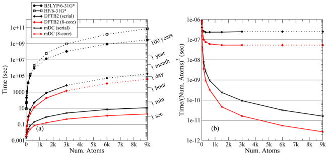
SCF evaluation timings for spheres of water of various sizes. (a) Timings shown on a log-scale. (b) Timings divided by the cube of the number of atoms. Part (b) is meant to illustrate the size at which the matrix diagonalization begins to adversely dominate the performance of the SCF procedure. Solid lines: observed timings; dotted lines: extrapolated estimates. Black lines: serial evaluation; red lines: OpenMP parallelized with 8 threads on an 8-processing-core workstation. Squares: HF/6-31G* evaluated with PSI (Ref. 97); circles: B3LYP/6-31G* evaluated with GAMESS (Ref. 96); diamonds: standard DFTB2; X’s: mDC. The B3LYP calculations were performed on an AMD Opteron (Model 8356). All other calculations were performed on an Intel Xeon E5520 workstation.
Figure 5.
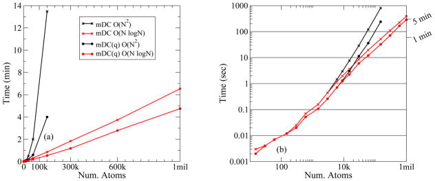
SCF evaluation timings for spheres of water of various sizes. (a) Timings shown on a linear-scale. (b) Timings shown on a double log-scale. Black lines: O(N2) brute-force electrostatics; red lines: O(N log N) adaptive FMM electrostatics. X’s: mDC with point multipoles; circles: mDC with point charges. All calculations were performed on an Intel Xeon E5520 workstation and performed using 8-cores.
3 Results and Discussion
3.1 The Effect of Intermolecular Tight-Binding Energy on the Water Dimer Geometry
Standard DFTB2 does a good job at reproducing the geometries and relative binding energies of water clusters. It is particularly impressive that DFTB2 predicts the correct geometry of the water dimer fairly accurately even though the explicit electrostatic interactions occur through monopolar charges only. When we remove the inter-water overlap and associated Fock matrix elements [mDC(q)], however, the hydrogen bond angle “flattens” in a manner similar to what one observes with the TIP3P water model (see Figure 3 and Table 1.) From this we infer that DFTB2 retains the proper dimer wag angle, not through a second order electrostatic interaction, but through the multipolar character of the two-center AO basis products and the resulting effect on the inter-region coupling through the tight-binding energy. Note, that despite getting a fairly accurate water dimer binding geometry, the water dimer adiabatic binding energy with DFTB2 is considerably under-bound by 2.8 kcal/mol relative to MP2 or 1.2 kcal/mol relative to MP2+CP.
We were interested to explore the possibility of creating a mDC method that improves the accuracy of the intermolecular interaction energies relative to DFTB2 while retaining good geometries. Initial tests using models based on monopolar charge representations for the second-order term, while able in some cases to obtain improved energies, were not successful in reliably reproducing the dimer (and cluster) geometries. The solution to the geometry problem came upon considering models that included higher-order multipole electrostatic interactions. Our approach was thus to expand the density matrix to higher-order atomic multipoles and use those expansions only for the inter-region interaction. Since these higher-order multipoles do not directly alter the intra-region energy, this strategy allows us to avoid having to reparametrize the DFTB2 model for intramolecular interactions, for which the model has proved to be highly successful, and instead concentrate on intermolecular interactions. The multipole expansions do indirectly affect the energy of a water through the variational procedure that allows coupling of electrostatic interactions (through the multipole expansions) with other water molecules. The variational inclusion of the multipole moment expansions allows us to compute the mDC analytic gradients accurately with simple formulas (see Table 2.)
It was found that expanding the oxygen density up to quadrupole terms was necessary to obtain improved water dimer angles. Adjusting the parameter reduces the “b” angle error (Table 1) from 29.8° [mDC(q)] to 1.1° (mDC). We choose not to reduce this error to zero so that we can better reproduce the binding energies and geometries of larger clusters (Sec. Section 3.2). The parameter was then adjusted to reproduce the long-range tail (ROO > 5 Å) of the water dimer (Figure 2). The tail of the water dimer is not exactly reproduced because we found that the relative energies of larger water clusters were benefited by slightly over-polarizing the mDC water. From this simple procedure, the dipole moments of the isolated waters are (D): 2.19 (MP2), 1.63 (DFTB2), and 2.34 (mDC); and the quadrupole moments are (a.u.): 2.14 (MP2), 1.11 (DFTB2), and 2.14 (mDC).
3.2 Reproduction of Water Cluster Relative Energies and Geometries
Table 3 compares DFTB2 and mDC water cluster geometries and relative energies to MP2, MP2+CP and 〈MP2〉. In general, DFTB2 does an excellent job of retaining the proper water cluster minima. Only a few DFTB2 clusters degenerate into lower energy clusters (e.g., 5HOH_Envelope) or other hydrogen bonding arrangements (e.g., 4HOH_7, 6HOH_Twisted_Boat, 6HOH_Intermediate_bag, 6HOH_Tricycle_1a, and 6HOH_Triple_trimer.) mDC does not rearrange the hydrogen bonds in any case where DFTB2 does not and retains the MP2 hydrogen bonding network in most cases where DFTB2 reorganizes. The exceptions to this are the 5HOH_Envelope and 6HOH_Intermediate_bag structures, which both DFTB2 and mDC undergo a reorganization.
Table 4 summarizes the ΔE and ΔΔE differences between the models. The mDC model reduces the ΔΔE unsigned error by factors of 1.7, 3.0, and 3.2 for tetramer, pentamer, and hexamer clusters, respectively when compared to MP2, and by factors of 2.5, 2.8, and 1.7 when compared to MP2+CP. The rms errors are also reduced by nearly a factor of two.
3.3 Computational Cost
Figure 4(a) displays timing results for ab initio, DFTB2, and mDC. For a 9 000 atom system, an ab initio SCF procedure would take 100 years to complete, assuming a cubic extrapolation of observed timings. Standard DFTB2 would take a day and mDC takes 2-to-10 seconds. Figure 4(b) re-displays the DFTB2 and mDC timings divided by the cube of the number of atoms. Therefore, the horizontal lines in this figure represent perfect O(N3) scaling. The DFTB2 timings become dominated by the O(N3) diagonalizations at around 600 atoms.
Overcoming the diagonalization bottleneck is only one obstacle toward achieving linear-scaling. Electrostatic interactions scale O(N2), but methods for its O(N log N) evaluation exist; e.g., various linear-scaling Ewald method for periodic systems99–102 and the FMM for non-periodic systems.98 Figure 5(a) compares the SCF timings between brute-force electrostatic with an adaptive FMM.98 The mDC timings with the FMM show linearity to one million atoms. We also show the timings for the mDC(q) model to measure the cost of including higher-order multipoles in the method. For large systems, the use of multipoles increases the cost by less than a factor of two. When comparing the timings between mDC and mDC(q), it is important to note that they differ only in their treatment of the electrostatic interactions, and the differences are not due to our modification of DFTB2 to expand the density to higher-order atomic multipoles. The atoms in mDC(q) continue to have point quadrupole moments and those expansions are still mapped from the density matrix and the potentials are reverse-mapped into the Fock matrix; it only so happens that the and parameters have been set to zero and the electrostatic interactions have been optimized for point-charges.
Figure 5(b) shows Figure 5(a) on a double-log scale to make the smaller systems more visible and show the points at which the FMM becomes faster than brute-force electrostatic evaluation. The “break-even” points, relative to full evaluation of electrostatic interactions, occur at 4 000 atoms (point multipoles) and 8 000 atoms (point charges). Prior to these system sizes, full electrostatic evaluation is quite efficient. To put the scale of Figure 5 into perspective, a desktop computer computed a one million atom system with mDC in 6.5 minutes. Assuming a cubic scaling, standard DFTB2 and B3LYP/6-31G* would take 1 700 years and 131 million years, respectively.
4 Conclusion
We have described a variational modified divide-and-conquer algorithm with charge-dependent inter-region interactions that eliminates the need for a buffer space, is extremely efficient, accurate and has simple gradient formulas. We have applied this method with the DFTB2 Hamiltonian and demonstrated that intermolecular interactions in the mDC method require higher-order multipole expansions to reproduce the correct geometry and binding for a broad range of water clusters. The resulting mDC model well-reproduces the reference MP2 quadrupole moment of water and greatly improves the binding energies and geometries of water clusters relative to the full DFTB2 method. This strategy allows intermolecular interactions to be tuned to obtain even higher accuracy than the DFTB2 method without sacrificing the quality of the intramolecular geometries and energies. This balance of intra- and intermolecular interactions may be important for the development of linear-scaling quantum mechanical force fields for molecular simulations. DFTB2 and mDC program execution timings were compared with ab initio programs using modestly simple Hamiltonians, from which the performance of mDC was shown to be superior. It was shown that a complete SCF calculation of a 3,000 atom system, using quadrupole expansions and the FMM, takes 0.44 seconds, whereas a one million atom system was possible to calculate in 6.5 minutes.
Supplementary Material
Acknowledgments
The authors are grateful for financial support provided by the National Institutes of Health (GM084149). Computational resources from the Minnesota Supercomputing Institute for Advanced Computational Research (MSI) were utilized in this work. This research was supported in part by the National Science Foundation through TeraGrid resources provided by the National Center for Supercomputing Applications and the Texas Advanced Computing Center under grant TG-CHE100072.
Footnotes
Supporting Information Available
Parameters for the mDC model are provided in the supporting information.
This material is available free of charge via the Internet at http://pubs.acs.org/.
References
- 1.Lassila JK, Zalatan JG, Herschlag D. Annu Rev Biochem. 2011;80:669–702. doi: 10.1146/annurev-biochem-060409-092741. [DOI] [PMC free article] [PubMed] [Google Scholar]
- 2.Steinbrecher T, Koslowski T, Case DA. J Phys Chem B. 2008;112:16935–16944. doi: 10.1021/jp8076134. [DOI] [PMC free article] [PubMed] [Google Scholar]
- 3.Bressler C, Chergui M. Annu Rev Phys Chem. 2010;61:263–282. doi: 10.1146/annurev.physchem.012809.103353. [DOI] [PubMed] [Google Scholar]
- 4.Castner EW, Jr, Margulis CJ, Maroncelli M, Wishart JF. Annu Rev Phys Chem. 2011;62:85–105. doi: 10.1146/annurev-physchem-032210-103421. [DOI] [PubMed] [Google Scholar]
- 5.Barone V, Improta R, Rega N. Acc Chem Res. 2008;41:605–616. doi: 10.1021/ar7002144. [DOI] [PubMed] [Google Scholar]
- 6.Bühl M, van Mourik T. WIREs Comput Mol Sci. 2011;1:634–647. [Google Scholar]
- 7.Yang W. Phys Rev A. 1991;44:7823–7826. doi: 10.1103/physreva.44.7823. [DOI] [PubMed] [Google Scholar]
- 8.Yang W, Lee TS. J Chem Phys. 1995;103:5674–5678. [Google Scholar]
- 9.Scuseria GE, Ayala PY. J Chem Phys. 1999;111:8330–8343. [Google Scholar]
- 10.Shao Y, White CA, Head-Gordon M. J Chem Phys. 2001;114:6572–6577. [Google Scholar]
- 11.Morokuma K. Phil Trans R Soc Lond A. 2002;360:1149–1164. doi: 10.1098/rsta.2002.0993. [DOI] [PubMed] [Google Scholar]
- 12.Goedecker S, Scuseria GE. IEEE Comput Sci Eng. 2003;5:14–21. [Google Scholar]
- 13.He X, Zhang JZH. J Chem Phys. 2006;124:184703. doi: 10.1063/1.2194535. [DOI] [PubMed] [Google Scholar]
- 14.Gogonea V, Suárez D, van der Vaart A, Merz KM., Jr Curr Opin Struct Biol. 2001;11:217–223. doi: 10.1016/s0959-440x(00)00193-7. [DOI] [PubMed] [Google Scholar]
- 15.Lewis JP, Liu S, Lee TS, Yang W. J Comput Phys. 1999;151:242–263. [Google Scholar]
- 16.Khandogin J, York DM. J Phys Chem B. 2002;106:7693–7703. [Google Scholar]
- 17.Monard G, Bernal-Uruchurtu MI, van der Vaart A, Merz KM, Jr, Ruiz-López MF. J Phys Chem A. 2005;109:3425–3432. doi: 10.1021/jp0459099. [DOI] [PubMed] [Google Scholar]
- 18.Shao Y, et al. Phys Chem Chem Phys. 2006;8:3172–3191. doi: 10.1039/b517914a. [DOI] [PubMed] [Google Scholar]
- 19.Hu H, Lu Z, Elstner M, Hermans J, Yang W. J Phys Chem A. 2007;111:5685–5691. doi: 10.1021/jp070308d. [DOI] [PMC free article] [PubMed] [Google Scholar]
- 20.Zhou T, Huang D, Caflisch A. Curr Top Med Chem. 2010;10:33–45. doi: 10.2174/156802610790232242. no pdf. [DOI] [PubMed] [Google Scholar]
- 21.Hu X, Jin Y, Zeng X, Hu H, Yang W. Phys Chem Chem Phys. 2012;14:7700–7709. doi: 10.1039/c2cp23714h. [DOI] [PMC free article] [PubMed] [Google Scholar]
- 22.He X, Merz KM., Jr J Chem Theory Comput. 2010;6:405–411. doi: 10.1021/ct9006635. [DOI] [PMC free article] [PubMed] [Google Scholar]
- 23.Vydrov OA, Van Voorhis T. J Chem Theory Comput. 2012;8:1929–1934. doi: 10.1021/ct300081y. [DOI] [PubMed] [Google Scholar]
- 24.Kobayashi M, Kunisada T, Akama T, Sakura D, Nakai H. J Chem Phys. 2011;134:034105. doi: 10.1063/1.3524337. [DOI] [PubMed] [Google Scholar]
- 25.Giese TJ, York DM. J Chem Phys. 2007;127:194101. doi: 10.1063/1.2778428. [DOI] [PubMed] [Google Scholar]
- 26.Elstner M, Porezag D, Jungnickel G, Elsner J, Haugk M, Frauenheim T, Suhai S, Seifert G. Phys Rev B. 1998;58:7260–7268. [Google Scholar]
- 27.Gao J. J Phys Chem. 1997;101:657–663. [Google Scholar]
- 28.Gao J. J Chem Phys. 1998;109:2346–2354. [Google Scholar]
- 29.Xie W, Gao J. J Chem Theory Comput. 2007;3:1890–1900. doi: 10.1021/ct700167b. [DOI] [PMC free article] [PubMed] [Google Scholar]
- 30.Gresh N, Cisneros GA, Darden TA, Piquemal JP. J Chem Theory Comput. 2007;3:1960–1986. doi: 10.1021/ct700134r. [DOI] [PMC free article] [PubMed] [Google Scholar]
- 31.Gresh N, Claverie P, Pullman A. Theor Chem Acc. 1984;66:1–20. [Google Scholar]
- 32.Piquemal J, Cisneros G, Reinhardt P, Gresh N, Darden TA. J Chem Phys. 2006;124:104101. doi: 10.1063/1.2173256. [DOI] [PMC free article] [PubMed] [Google Scholar]
- 33.Cisneros GA, Piquemal J, Darden TA. J Chem Phys. 2006;125:184101. doi: 10.1063/1.2363374. [DOI] [PMC free article] [PubMed] [Google Scholar]
- 34.Cisneros GA, Elking D, Piquemal JP, Darden TA. J Phys Chem A. 2007;111:12049–12056. doi: 10.1021/jp074817r. [DOI] [PMC free article] [PubMed] [Google Scholar]
- 35.Cisneros GA, Darden TA, Gresh N, Reinhardt P, Parisel O, Pilmé J, Piquemal J-P. Chapter Design of next generation force fields from ab initio computations: Beyond point charges electrostatics. Springer Verlag; 2009. Multi-scale quantum models for biocatalysis; pp. 137–172. [Google Scholar]
- 36.Schwegler E, Challacombe M. J Chem Phys. 1999;111:6223–6229. [Google Scholar]
- 37.Challacombe M. J Chem Phys. 2000;113:10037–10043. [Google Scholar]
- 38.Beck TL. Rev Mod Phys. 2000;72:1041–1080. [Google Scholar]
- 39.Watson MA, Sałek P, Macak P, Helgaker T. J Chem Phys. 2004;121:2915–2931. doi: 10.1063/1.1771639. [DOI] [PubMed] [Google Scholar]
- 40.White CA, Johnson BG, Gill PMW, Head-Gordon M. Chem Phys Lett. 1994;230:8–16. [Google Scholar]
- 41.Kutte R, Aprá E, Nichols J. Chem Phys Lett. 1995;238:173–179. [Google Scholar]
- 42.Burant JC, Strain MC, Scuseria GE, Frisch MJ. Chem Phys Lett. 1996;248:43–49. [Google Scholar]
- 43.Strain MC, Scuseria GE, Frisch MJ. Science. 1996;271:51–53. [Google Scholar]
- 44.Schwegler E, Challacombe M, Head-Gordon M. J Chem Phys. 1997;106:9708–9717. [Google Scholar]
- 45.Challacombe M, Schwegler E. J Chem Phys. 1997;106:5526–5536. [Google Scholar]
- 46.Jung Y, Sodt A, Gill PW, Head-Gordon M. Proc Natl Acad Sci. 2005;102:6692–6697. doi: 10.1073/pnas.0408475102. [DOI] [PMC free article] [PubMed] [Google Scholar]
- 47.Dahlke EE, Truhlar DG. J Chem Theory Comput. 2007;3:1342–1348. doi: 10.1021/ct700057x. [DOI] [PubMed] [Google Scholar]
- 48.Xie W, Song L, Truhlar DG, Gao J. J Chem Phys. 2008;128:234108. doi: 10.1063/1.2936122. [DOI] [PMC free article] [PubMed] [Google Scholar]
- 49.Xie W, Orozco M, Truhlar DG, Gao J. J Chem Theory Comput. 2009;5:459–467. doi: 10.1021/ct800239q. [DOI] [PMC free article] [PubMed] [Google Scholar]
- 50.Isegawa M, Gao J, Truhlar DG. J Chem Phys. 2011;135:084107. doi: 10.1063/1.3624890. [DOI] [PMC free article] [PubMed] [Google Scholar]
- 51.Zhang P, Truhlar DG, Gao J. Phys Chem Chem Phys. 2012;14:7821–7829. doi: 10.1039/c2cp23758j. [DOI] [PMC free article] [PubMed] [Google Scholar]
- 52.Wang Y, Sosa CP, Cembran A, Truhlar DG, Gao J. J Phys Chem B. 2012;116:6781–6788. doi: 10.1021/jp212399g. [DOI] [PMC free article] [PubMed] [Google Scholar]
- 53.Gao J, Wang Y. J Chem Phys. 2012;136:071101. doi: 10.1063/1.3688232. [DOI] [PMC free article] [PubMed] [Google Scholar]
- 54.Cembran A, Bao P, Wang Y, Song L, Truhlar DG, Gao J. J Chem Theory Comput. 2010;6:2469–2476. doi: 10.1021/ct100268p. [DOI] [PMC free article] [PubMed] [Google Scholar]
- 55.Jacobson LD, Herbert JM. J Chem Phys. 2011;134:094118. doi: 10.1063/1.3560026. [DOI] [PubMed] [Google Scholar]
- 56.Kitaura K, Ikeo E, Asada T, Nakano T, Uebayasi M. Chem Phys Lett. 1999;313:701–706. [Google Scholar]
- 57.Nagata T, Brorsen K, Fedorov DG, Kitaura K, Gordon MS. J Chem Phys. 2011;134:124115. doi: 10.1063/1.3568010. [DOI] [PubMed] [Google Scholar]
- 58.Pruitt SR, Fedorov DG, Kitaura K, Gordon MS. J Chem Theory Comput. 2010;6:1–5. doi: 10.1021/ct900442b. [DOI] [PubMed] [Google Scholar]
- 59.Nagata T, Fedorov1 DG, Kitaura K, Gordon MS. J Chem Phys. 2009;131:024101–024112. doi: 10.1063/1.3156313. [DOI] [PubMed] [Google Scholar]
- 60.Fedorov DG, Kitaura K. J Phys Chem A. 2007;111:6904–6914. doi: 10.1021/jp0716740. [DOI] [PubMed] [Google Scholar]
- 61.Fedorov DG, Olson RM, Kitaura K, Gordon MS, Koseki S. J Comput Chem. 2004;25:872–880. doi: 10.1002/jcc.20018. [DOI] [PubMed] [Google Scholar]
- 62.Nakano T, Kaminuma T, Sato T, Fukuzawa K, Akiyama Y, Uebayasi M, Kitaura K. Chem Phys Lett. 2002;351:475–480. [Google Scholar]
- 63.Le HA, Tan HJ, Ouyang JF, Bettens RPA. J Chem Theory Comput. 2012;8:469–478. doi: 10.1021/ct200783n. [DOI] [PubMed] [Google Scholar]
- 64.Elliott P, Cohen MH, Wasserman A, Burke K. J Chem Theory Comput. 2009;5:827–833. doi: 10.1021/ct9000119. [DOI] [PubMed] [Google Scholar]
- 65.Mayhall NJ, Raghavachari K. J Chem Theory Comput. 2012;8:2669–2675. doi: 10.1021/ct300366e. [DOI] [PubMed] [Google Scholar]
- 66.Yang W. J Mol Struct. 1992;255:461–479. [Google Scholar]
- 67.Ammar GS, Reichel L, Sorensen DC. ACM Trans Math Soft. 1992;18:292–307. [Google Scholar]
- 68.Lee C, Yang W. J Chem Phys. 1992;96:2408–2411. [Google Scholar]
- 69.Zhao Q, Yang W. J Chem Phys. 1995;102:9598–9603. [Google Scholar]
- 70.Dixon SL, Merz KM., Jr J Chem Phys. 1996;104:6643–6649. [Google Scholar]
- 71.Lee TS, York DM, Yang W. J Chem Phys. 1996;105:2744–2750. [Google Scholar]
- 72.York DM, Lee TS, Yang W. J Am Chem Soc. 1996;118:10940–10941. [Google Scholar]
- 73.Dixon SL, Merz KM., Jr J Chem Phys. 1997;107:879–893. [Google Scholar]
- 74.Pan W, Lee TS, Yang W. J Comput Chem. 1998;19:1101–1109. [Google Scholar]
- 75.Lee TS, Yang W. Int J Quantum Chem. 1998;69:397–404. [Google Scholar]
- 76.van der Vaart A, Suárez D, Merz KM., Jr J Chem Phys. 2000;113:10512–10523. [Google Scholar]
- 77.van der Vaart A, Valentin G, Dixon SI, Merz KM., Jr J Comput Chem. 2000;21:1494–1504. [Google Scholar]
- 78.Frauenheim T, Seifert G, Elstner M, Niehaus T, Köhler C, Amkreutz M, Sternberg M, Hajnal Z, Di Carlo A, Suhai S. J Phys: Condens Matter. 2002;14:3015–3047. [Google Scholar]
- 79.Wollacott AM, Merz KM., Jr J Chem Theory Comput. 2007;3:1609–1619. doi: 10.1021/ct600325q. [DOI] [PMC free article] [PubMed] [Google Scholar]
- 80.Song GL, Li ZH, Liu ZP, Cao XM, Wang W, Fan KN, Xie Y, Schaefer HF., III J Chem Theory Comput. 2008;4:2049–2056. doi: 10.1021/ct800265p. [DOI] [PubMed] [Google Scholar]
- 81.Kobayashi M, Nakai H. J Chem Phys. 2009;131:114108. doi: 10.1063/1.3211119. [DOI] [PubMed] [Google Scholar]
- 82.Alizadegan R, Hsia KJ, Martinez TJ. J Chem Phys. 2010;132:034101. doi: 10.1063/1.3290949. [DOI] [PubMed] [Google Scholar]
- 83.Zhu T, He X, Zhang JZH. Phys Chem Chem Phys. 2012;14:7837–7845. doi: 10.1039/c2cp23746f. [DOI] [PubMed] [Google Scholar]
- 84.Giese TJ, York DM. J Chem Phys. 2008;129:016102. doi: 10.1063/1.2945897. [DOI] [PMC free article] [PubMed] [Google Scholar]
- 85.Elstner M, Frauenheim T, Kaxiras E, Seifert G, Suhai S. Phys Status Solidi B. 2000;217:357–376. [Google Scholar]
- 86.Yang Y, Yu H, York D, Elstner M, Qiang C. J Chem Theory Comput. 2008;4:2067–2084. doi: 10.1021/ct800330d. [DOI] [PMC free article] [PubMed] [Google Scholar]
- 87.Kaminski S, Gaus M, Phatak P, von Stetten D, Elstner M, Mroginski MA. J Chem Theory Comput. 2010;6:1240–1255. [Google Scholar]
- 88.Gaus M, Cui Q, Elstner M. J Chem Theory Comput. 2011;7:931–948. doi: 10.1021/ct100684s. [DOI] [PMC free article] [PubMed] [Google Scholar]
- 89.Pellenq R, Nicholson D. Mol Phys. 1998;95:549–570. [Google Scholar]
- 90.Giese TJ, York DM. J Chem Phys. 2011;134:194103. doi: 10.1063/1.3587052. [DOI] [PMC free article] [PubMed] [Google Scholar]
- 91.Giese TJ, York DM. Theor Chem Acc. 2012;131:1145. doi: 10.1007/s00214-012-1145-7. [DOI] [PMC free article] [PubMed] [Google Scholar]
- 92.Giese TJ, York DM. J Chem Phys. 2008;128:064104. doi: 10.1063/1.2821745. [DOI] [PMC free article] [PubMed] [Google Scholar]
- 93.Frisch MJ, et al. Gaussian 09, Revision A.02. Gaussian, Inc; Wallingford, CT: 2009. [Google Scholar]
- 94.Dyke TR, Mack KM, Muenter JS. J Chem Phys. 1977;66:498–510. [Google Scholar]
- 95.Klopper W, van Duijneveldtvan de Rijdt JGCM, van Duijneneldt FB. Phys Chem Chem Phys. 2000;2:2227–2234. [Google Scholar]
- 96.Schmidt MW, Baldridge KK, Boatz JA, Elbert ST, Gordon MS, Jensen JH, Koseki S, Matsunaga N, Nguyen KA, Su S, Windus TL, Dupuis M, John A, Montgomery J. J Comput Chem. 1993;14:1347–1363. [Google Scholar]
- 97.Crawford TD, Sherrill CD, Valeev EF, Fermann JT, King RA, Leininger ML, Brown ST, Janssen CL, Seidl ET, Kenny JP, Allen WD. J Comput Chem. 2007;28:1610–1616. doi: 10.1002/jcc.20573. [DOI] [PubMed] [Google Scholar]
- 98.Giese TJ, York DM. J Comput Chem. 2008;29:1895–1904. doi: 10.1002/jcc.20946. [DOI] [PMC free article] [PubMed] [Google Scholar]
- 99.Darden T, York D, Pedersen L. J Chem Phys. 1993;98:10089–10092. [Google Scholar]
- 100.York DM, Yang W. J Chem Phys. 1994;101:3298–3300. [Google Scholar]
- 101.Sagui C, Darden TA. Annu Rev Biophys Biomol Struct. 1999;28:155–179. doi: 10.1146/annurev.biophys.28.1.155. [DOI] [PubMed] [Google Scholar]
- 102.Nam K, Gao J, York DM. J Chem Theory Comput. 2005;1:2–13. doi: 10.1021/ct049941i. [DOI] [PubMed] [Google Scholar]
Associated Data
This section collects any data citations, data availability statements, or supplementary materials included in this article.