Stability selection for regression-based models of transcription factor–DNA binding specificity

Abstract

Motivation: The DNA binding specificity of a transcription factor (TF) is typically represented using a position weight matrix model, which implicitly assumes that individual bases in a TF binding site contribute independently to the binding affinity, an assumption that does not always hold. For this reason, more complex models of binding specificity have been developed. However, these models have their own caveats: they typically have a large number of parameters, which makes them hard to learn and interpret.

Results: We propose novel regression-based models of TF–DNA binding specificity, trained using high resolution in vitro data from custom protein-binding microarray (PBM) experiments. Our PBMs are specifically designed to cover a large number of putative DNA binding sites for the TFs of interest (yeast TFs Cbf1 and Tye7, and human TFs c-Myc, Max and Mad2) in their native genomic context. These high-throughput quantitative data are well suited for training complex models that take into account not only independent contributions from individual bases, but also contributions from di- and trinucleotides at various positions within or near the binding sites. To ensure that our models remain interpretable, we use feature selection to identify a small number of sequence features that accurately predict TF–DNA binding specificity. To further illustrate the accuracy of our regression models, we show that even in the case of paralogous TF with highly similar position weight matrices, our new models can distinguish the specificities of individual factors. Thus, our work represents an important step toward better sequence-based models of individual TF–DNA binding specificity.

Availability: Our code is available at http://genome.duke.edu/labs/gordan/ISMB2013. The PBM data used in this article are available in the Gene Expression Omnibus under accession number GSE47026.

Contact: raluca.gordan@duke.edu

1 INTRODUCTION

At the level of transcription, gene expression is regulated mainly via the binding of transcription factors (TFs) to specific short DNA sites in the promoters or enhancers of genes they regulate. Accurate characterization of the DNA binding specificity of TFs is critical to understand how these proteins achieve their regulatory purpose in the cell. Currently, the most widely used model for representing the DNA binding specificity of a TF is the position weight matrix (PWM, or DNA motif) (Staden, 1984; Stormo, 2000), a matrix containing scores (or weights) for each nucleotide at every position in the TF binding site. PWMs can perform well in practice: these models have been combined with chromatin accessibility data to successfully predict where specific TFs bind across the genome in a cell-specific way (Kaplan et al., 2011; Pique-Regi et al., 2011). However, PWM models make the assumption that individual bases in a TF binding site contribute independently and additively to the affinity of that site, which is not always true in practice.

Dependencies among positions within TF binding sites have been observed in small-scale experimental studies (Bulyk et al., 2002; Jauch et al., 2012; Man and Stormo, 2001), in statistical analyses of known TF binding sites (Tomovic and Oakeley, 2007; Zhou and Liu, 2004), and in computational analyses of high-throughput in vitro and in vivo TF binding data (Badis et al., 2009; Berger et al., 2006; Jolma et al., 2013; Zhao et al., 2012). This suggests that extending the classic definition of a PWM may lead to specificity models that better fit the TF binding data. Indeed, several studies have explored more complex models of TF–DNA binding specificity and found that they outperform PWMs (Barash et al., 2003; Siddharthan, 2010). However, complex models are typically characterized by a large number of parameters, which makes them hard to interpret (Agius et al., 2010; Annala et al., 2011) and prone to overfitting (Zhou and Liu, 2004).

Here, we present regression-based models of TF–DNA binding specificity, which take into account both the contributions from individual bases in a TF binding site and the contributions from higher-order k-mers. Our approach differs from previous work in three aspects: (i) our models are trained on high-throughput quantitative data generated specifically for this task; (ii) we use a new feature selection method based on LASSO regression (Bach, 2008; Meinshausen and Bühlmann, 2010; Tibshirani, 1996) to restrict the number of features, which makes our models easier to visualize and interpret; and (iii) we include dependencies by using 2-mers and 3-mers as features and by using a non-linear support vector regression (SVR) method. The first aspect is important because many previous models were trained either on a small number of high-resolution binding regions (Barash et al., 2003; Zhou and Liu, 2004) or on high-throughput in vivo data (Sharon et al., 2008; Siddharthan, 2010), both of which are noisy, have low resolution and may reflect both direct and indirect DNA binding of the tested TFs (Gordân et al., 2009). In vitro data from high-throughput assays—such as protein binding microarrays (PBMs) (Berger et al., 2006), MITOMI (Maerkl and Quake, 2007) or high-throughput SELEX (Jolma et al., 2010; Zhao et al., 2009)—are more appropriate for learning complex models of TF–DNA binding specificity (Agius et al., 2010; Annala et al., 2011; Weirauch et al., 2013; Zhao et al., 2009). Here, we use the PBM technology to generate custom data on the binding specificities of the TFs of interest. Our microarray designs contain hundreds or thousands of genomic DNA regions centered at putative DNA binding sites for the TFs of interest (see Section 2 for details).

The features used in our regression models are based on the occurrences of 1-mers, 2-mers and 3-mers at various positions in the TF binding sites or their flanking regions. Regression models that take into account all k-mers have hundreds or thousands of parameters, depending on the value of k and on the size of the flanking regions. Such a large number of parameters can lead to overfitting the training data and also make the models hard to visualize and interpret. To overcome this problem, we use a feature selection approach based on LASSO regression (Bach, 2008; Haury et al., 2012; Meinshausen and Bühlmann, 2010; Tibshirani, 1996). This allows us to drastically reduce the number of parameters to estimate while maintaining high prediction accuracy.

To illustrate the accuracy of our regression models, we train and test them on custom PBM data for five TFs from the bHLH protein family: yeast TFs Cbf1 and Tye7, and human TFs c-Myc (‘Myc’), Max and Mad2 (‘Mad’). We show that for both yeast and human bHLH TFs, our regression models can distinguish the binding specificities of individual family members, although their PWMs (Fig. 1) are highly similar. This illustrates that our approach may be used to better understand the importance of intrinsic sequence preferences for achieving specificity within TF families.

Fig. 1.

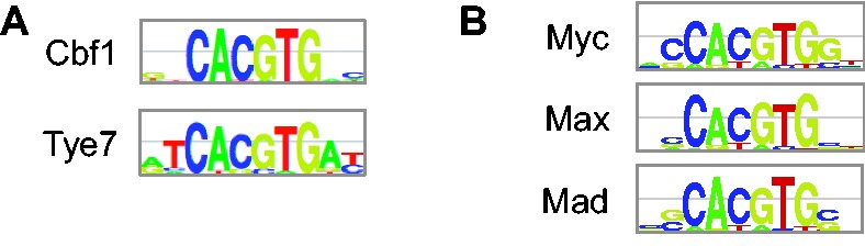
PWMs for yeast TFs Cbf1 and Tye7 (A) and human TFs Myc, Max and Mad (B). PWMs were derived from universal PBM data [Munteanu and Gordân, 2013 (B); Zhu et al., 2009 (A)], and PWM logos were generated using enoLOGOS (Workman et al., 2005). As Myc and Mad do not bind DNA efficiently on their own, the Myc and Mad PBM experiments were performed using each TF in combination with Max (see Section 3.1)

2 APPROACH

Our approach for learning TF–DNA binding specificity models is summarized in Figure 2. We design custom microarrays that contain genomic regions centered at putative TF binding sites. Next, we measure TF binding to the selected genomic regions, using the PBM technology (Berger and Bulyk, 2009). Briefly, in a PBM experiment, we express each TF of interest with an epitope tag (typically a GST or 6xHis tag), purify it and apply it to a double-stranded DNA microarray. After the TF binds its preferred sequences on the microarray, we label the microarray with a fluorophore-conjugated antibody specific for the protein tag. Next, the microarray is scanned to generate a fluorescence intensity value for each DNA sequence present on the array. Higher intensities correspond to DNA sequences with higher affinities for the TF.

Fig. 2.

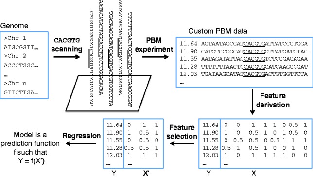
Workflow of the proposed method for learning the DNA binding specificity of TFs using custom PBMs

The vast majority of PBM data available in the literature have been generated using ‘universal’ array designs, which contain artificial DNA sequences designed to collectively cover all possible 10-mers (Berger et al., 2006). Thus, universal PBM data provide a broad, unbiased view of the DNA binding preferences of TFs. However, universal PBM data are not suitable to predict binding of a TF to longer genomic sequences. To overcome this problem, we designed custom ‘genomic’ arrays to directly measure TF binding of putative DNA binding sites in native genomic context.

The DNA sequences on our custom microarrays were designed to include a large number of potential DNA binding sites for the TFs of interest. To learn the DNA binding specificities of Cbf1 and Tye7, we used custom PBM data from Gordân et al. (2013). For Myc, Max and Mad, we designed a new array containing potential Myc/Max/Mad binding sites extracted from the human genome. As all bHLH TFs used in this study are known to have a strong preference for the E-box CACGTG, both the Cbf1/Tye7 and the Myc/Max/Mad array designs focus on the genomic sites centered at this E-box (Fig. 2).

From the raw PBM data, we compute the natural logarithm of the normalized signal intensity for each DNA sequence containing the E-box CACGTG flanked by genomic sequences of 12 or 15 bases on each side for Cbf1/Tye7 and Myc/Max/Mad, respectively. Next, we derive quantitative features from the sequence content of the genomic regions flanking the CACGTG E-box core, and we use them to train regression models that can predict the PBM signal intensity (i.e. the in vitro TF–DNA binding specificity). Our custom PBM data allow us to investigate whether the genomic flanks of the E-box sites influence binding affinity differently for distinct members of the same TF family.

Regression-based approaches are a natural fit for the continuous intensity data from PBM experiments. The purpose of a regression model is to estimate a function f to fit the output y to the input features X as . In our case, y is the binding intensity as measured on the microarray and X are DNA sequence features. In particular, to introduce dependency effects, we take X to be all individual nucleotides, and all pairs, triplets and quadruplets of sequential nucleotides (2-mers, 3-mers and 4-mers) in the DNA sequences in our training set. A good candidate function is expected to fit the training set well (i.e. y close to f(X)) and to produce accurate predictions on new test examples (i.e. low generalization error). The latter is usually assessed by cross-validation experiments, where part of the dataset is used to learn the regression function, which is used to predict the output y on the held out part.

When X is of high dimension, regularization is a standard practice, which consists in smoothing function f to ensure low generalization error and to prevent overfitting. One method of regularization, known as ‘feature selection’, is to select a small subset of features that are sufficient to model the data. We note that our DNA sequence features result in high-dimensional features, which support the use of feature selection. Feature selection lends a model interpretability, by basing predictions on a small number of features that may have biological meaning, which is a desirable property when one wants to study further which features contribute to model accuracy.

Two popular regression methods are SVR (Smola and Schölkopf, 2004) and LASSO regression (Tibshirani, 1996). SVR often has good generalization error properties and, when used with a non-linear kernel, can capture non-linear functions f. LASSO regression includes an L₁ constraint that selects a small subset of features in X to explain the y variable and is preferred for interpretability purposes. However, the feature set selected by LASSO is not robust, even to slight perturbations of the data. This lack of stability casts doubt on the relevance of the subset of variables it selects. Following previous work (Bach, 2008; Haury et al., 2012; Meinshausen and Bühlmann, 2010) on ‘stability selection’, we propose a regression scheme that combines SVR and a stable feature selection procedure based on LASSO. We describe our methodology in detail in Section 3 and show the performance of our models on human and yeast TF binding data in Section 4.

3 METHODS

3.1 PBM data

Custom PBM data for Cbf1 and Tye7, in the form of normalized log signal intensity values, were obtained from Gordân et al. (2013). For Myc, Max and Mad, we performed PBM experiments (Berger and Bulyk, 2009) using 6xHis-tagged proteins expressed and purified in bacteria (as described in Lin et al., 2012). As Myc requires heterodimerization with Max to bind DNA efficiently, the Myc PBM experiments were performed using both Myc and Max on the same microarray. As in previous work (Munteanu and Gordân, 2013), we used a 10 times higher concentration of Myc compared with Max to ensure that mostly Myc:Max heterodimers, instead of Max:Max homodimers, are formed. Similarly, Mad PBM experiments were performed using both Mad and Max on the same microarray, with a 10 times higher concentration of Mad.

The Myc/Max/Mad custom array contains, in addition to positive and negative control sequences, 36-bp long human genomic regions centered at CACGTG sites. After scanning the microarray and normalizing the raw PBM data (as described in Berger and Bulyk, 2009), we compute, for each genomic sequence, the median log signal intensity over the six replicate spots that contain that particular sequence. These median log intensity values are used by the regression algorithms. In addition, to test the reproducibility of our PBM data, we performed replicate PBM experiments for TF Myc. We obtained a Pearson correlation coefficient (R) of 0.98 between replicate experiments.

Before training regression models using the custom PBM data, we filtered out any sequence that contained potential TF binding sites in the regions flanking the CACGTG core, to ensure that each sequence contains one and only one TF binding site. We required that the flanks do not contain any 8-mer with a PBM enrichment score (E-score) greater than 0.3. PBM E-scores range from −0.5 to +0.5, with higher values corresponding to higher sequence preferences; typically, E-scores > 0.35 correspond to specific TF–DNA binding (Berger et al., 2006; Gordân et al., 2011). After the filtering step, we obtained 280 sequences for Cbf1, 312 for Tye7, 4917 for Myc, 4430 for Max and 4292 for Mad. As expected, the number of sequences for each TF is much higher for the human TFs as compared with yeast TFs.

For each TF, we use N to denote the number of DNA sequences selected from the custom PBM data. The averaged DNA binding intensities (as measured on the PBMs) are the output that we aim to predict using regression models.

3.2 Feature derivation

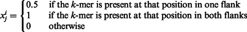
It is commonly accepted that much of the binding specificity of a protein-DNA complex is encoded in the base content of the DNA sequence. Therefore, our regression methods use sequence-based features. Numeric features are derived from sequences as follows. bHLH TFs typically bind DNA as dimers, i.e. two copies of the same protein or related proteins interact to bind two symmetric half-sites. Thus, as there is no way to define a ‘left’ versus a ‘right’ flank, we describe the base content of the two flanks simultaneously. To do so, we define the flanks as a single sequence using the palindromic symmetry of the E-box as shown in Figure 3. For each position flanking CACGTG, from 1 to 12 for Cbf1/Tye7 or 1 to 15 for Myc/Max/Mad, we count the occurrences of each k-mer, where . We obtain n vectors describing the sequences 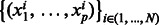where:

The index j refers to one k-mer at a particular position. p is therefore the product between the length of the flanking sequence and the number of k-mers used (see Table 1 for values of p). More precisely, a feature value of 1 means the corresponding k-mer is present in one flank at the corresponding position, and its complementary k-mer is present in the other flank at the same position. We eliminate those k-mer features that are completely absent from all sequences.

Fig. 3.

DNA regions flanking the CACGTG E-box are used to derive sequence-based features that take into account the dimer mode of DNA binding by bHLH proteins

Table 1.

Total number of features for different feature sets

Values of k	1	2	3	4	1–2	1–3	1–4
Cbf1	48	176	623	1596	224	847	2440
Tye7	48	176	624	1672	224	848	2520
Myc/Max/Mad	60	—	—	—	284	1116	—

We note that Cbf1, Tye7 and Max bind DNA efficiently as homodimers, i.e. using two copies of the same protein, whereas Myc and Mad need to heterodimerize with Max. Thus, in the case of Myc and Mad, only one of the half-sites is bound by the TF of interest, whereas the other is bound by the TF partner (Max). Ideally, one would treat the two half-sites differently and learn one model for each half-site; however, we do not know a priori, for each binding region, which half-site is bound by which TF. For this reason, for Myc and Mad, we use the same approach as for homodimers, recognizing that the specificity signal will be diluted because of the heterodimerization with Max.

3.3 Feature selection with ‘Stable LASSO’

LASSO regression enables feature selection through the use of an L₁ penalty. In particular, the output y is modeled as a linear function of the input features X by estimating the coefficient vector that minimizes the squared residual error plus the (scaled) absolute value of the coefficient weights, inducing many of the weights to go to zero, and effectively eliminating the use of that feature in prediction. We can write LASSO regression as the following optimization problem:

Parameter λ reflects the trade-off between fit and sparsity, or the proportion of features removed. The penalty term means that a solution w becomes sparser as λ increases. Thus, a smaller set of features are used to model y.

The least angle regression (LARS) algorithm (Efron et al., 2004) allows us to compute the solution path for all values of λ. This iterative algorithm adds features to the linear model one by one and exploits the fact that the w coefficients vary continuously as λ increases. A good value for λ is often chosen by cross-validation; instead, we keep the whole solution path, in a stability selection procedure described later in the text.

LASSO regression is sensitive to perturbations of the training set and often does not result in a robust set of selected features. This is especially true when the features are correlated, as is the case here because of redundancy between k-mers of different lengths. As the coefficient values estimated for each feature are unstable, they cannot be used directly as importance scores for features. To overcome those limitations, Bach (2008); Haury et al. (2012) and Meinshausen and Bühlmann (2010) have proposed the use of a stability selection procedure. This consists in randomly perturbing the dataset many times, running LASSO on those perturbed datasets and combining the successive regressions to obtain importance scores for each feature, based on the frequency with which they are selected in the successive LASSO runs. Such a score is akin to a probability that the feature should participate in the model.

Algorithm 1 Stable LASSO.

INPUT: = perturbation level, T = number of iterations

OUTPUT: An area score for all features

for t = 1 to T do

 Randomly perturb the data:

  Draw a subsample (y_t, X_t) of size n/2 from (y, X)

  Draw a vector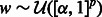

  Re-weight the features:

 Compute the LASSO path of length n/2 using LARS

 Keep the selection matrix where

end for

Compute the area score for feature i as

As described in Algorithm 1, at each iteration t = 1 … T, we perturb the original training set (y, X): we randomly subsample one half of the training set (y_t, X_t) and reweight all features in X_t using randomly generated weights w drawn uniformly on [α, 1]. Parameter α controls the level of perturbation: a smaller α implies more variable weights, whereas α = 1 means no reweighting.

In practice, instead of a loop of length T as shown in Algorithm 1, we run a single loop of length T/2 and compute the LARS path on the two random halves of the dataset at each iteration. This still allows us to compute the ‘area score’ (i.e. the feature importance score) as the average of T selection frequency matrices, as shown in Figure 4. The area score can be interpreted as the area under the average selection frequency curve over T iterations (see Fig. 5).

Fig. 4.

Output of Algorithm 1: T binary matrices describing which features are selected along the LARS path

Fig. 5.

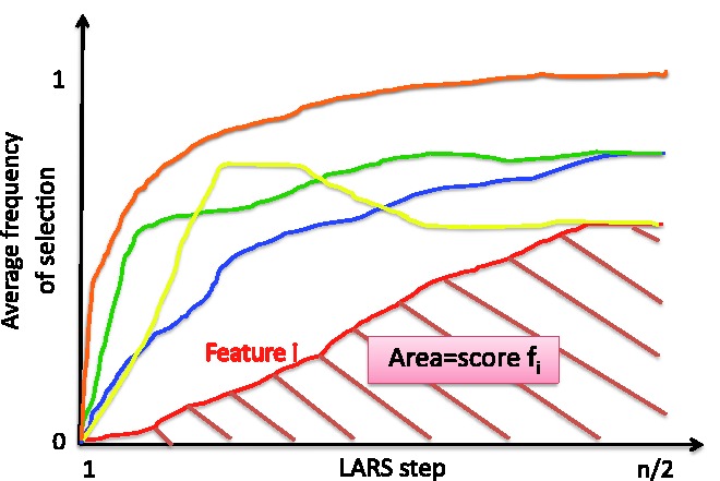
Computation of the ‘area score’ for each variable. An average selection frequency curve over the T iterations is computed for each feature (five features are shown in this figure). The area under each curve represents the area score for the corresponding feature

In the classic version of LASSO regression, one needs to select a value for parameter λ. Instead, the area score uses the whole regularization path and therefore has the great advantage of avoiding any arbitrary cutoff on the number of features and any additional computation time owing to parameter selection.

We observed that the area scores were distributed according to a multimodal distribution, each model corresponding to a given k-mer length. This suggests we cannot apply a single uniform threshold on the importance score across all features with different values of k. Instead, we derive one threshold value for each group of features of the same length. To do so, we computed a background score distribution for each k-mer length by randomly permuting the intensity values and running Stable LASSO on the permuted values. We then select features with an area score higher than the mean plus two standard deviations of their corresponding background distribution. Finally, we use this feature subset as input to an SVR to learn binding specificity models. In Section 4, we show that this Stable LASSO selection procedure performs better than simply choosing a small number of features (random selection) or choosing features based on their SVR weights (SVR selection) (see Fig. 7).

Fig. 7.

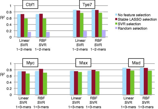
Predicting binding intensity for Cbf1, Tye7, Myc, Max and Mad using a regression-based model trained on selected features. The squared correlation coefficient between predicted intensity and actual intensity (y-axis) is computed for different feature selection strategies followed by a linear and an RBF SVR. Feature selection on 1–2-mers performed best for Cbf1 and Tye7. Feature selection on 1–3-mers performed best for Myc, Max and Mad TFs. A Wilcoxon paired signed rank test shows a significant difference between 1–2-mers and 1–3-mers, with P-values {0.002, 0.002, 0.0059}, respectively

3.4 Regression with SVR

SVR (Smola and Schölkopf, 2004) uses the concept of maximum margin (Vapnik, 1998) for regression. SVR is formulated as an optimization problem as follows:

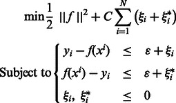The only difference between the SVR and the SVM lies in the loss function, which is devised for a continuous output in the case of the SVR. This loss function, called the ϵ-insensitive function, enforces the support vectors, or informative examples, to lie within a tube of width ϵ around function f. Parameter C orchestrates the trade-off between the loss term, which enforces a good fit to the training data, and the margin term, which regularizes the f function and often produces better generalization error. Parameter ϵ plays a similar role to C, with small values of ϵ leading to a better fit on the training set, and larger values preventing overfitting.

An essential ingredient to any SV method is the kernel function K, which can be thought of as a similarity function between any two example points. Function f can be written as 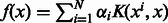The simplest kernel is the linear kernel, which is the dot product between the feature vectors for two samples:

implying f is linear in the input features x. Other kernels, however, yield a non-linear function f, via the ‘kernel trick’. This consists in defining an implicit mapping of the original features into a higher dimension space and looking for a linear function f in that transformed space. A common non-linear kernel is the radial basis function (RBF) kernel, defined by

The linear SVR allows us to associate coefficients to the features by rewriting f(x) so that coefficient for variable j is 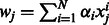However, the relationship between the features and the output is often better modeled by a non-linear (but not interpretable) kernel such as the RBF kernel.

Each model was evaluated by computing by computing the squared Pearson correlation coefficient (R²) between predicted DNA binding specificity/intensity and the actual PBM log signal intensity values.

4 RESULTS

4.1 Regression models trained on custom PBM data give accurate predictions of DNA binding specificity

We first evaluate the performance of full SVR regression models (i.e. without any feature selection) learned from yeast and human custom PBM data. To describe the DNA sequences, we used k-mers of different lengths and generated several features sets that included, successively, {1, 2, 3, 4, 1–2, 1–3, 1–4}-mers. Table 1 shows the resulting number of features (p) for different feature sets. Next, for each feature set, we ran a linear and an RBF SVR. We used 10-fold cross-validation for parameter selection over a large grid of possible parameter values. Each model was evaluated by computing the Pearson squared correlation coefficient (R²) between the predicted and the actual signal intensity of held out test data. For each method, a 10-fold cross validation was carried out to assess the performance in predicting binding specificity for test DNA sequences.

Figure 6 shows that the linear and RBF SVR model predictions are well correlated with the actual intensity. Among the regression models tested here, linear SVR models based on 1-mer features are technically equivalent to PWM models, including the assumption of independence and additivity. These models fit the data well and result in R² values of 0.6 or higher in the 10-fold cross-validation test. This is in agreement with previous studies suggesting that even when the additivity assumption does not fit the data perfectly, in many cases, it gives a good approximation of the data (Benos et al., 2002; Zhao and Stormo, 2011). However, taking into account non-independent contributions, by either using the RBF kernel or by incorporating 2-mer and 3-mer features, slightly improves the accuracy of our regression models trained on custom PBM data.

Fig. 6.

Performance (R²) of linear and RBF SVR regression methods (without feature selection) for learning binding specificity from sequence content. We used several feature sets to investigate the use of including longer k-mers in the models

Using 1-mers and 2-mers is enough to reach a good performance on Cbf1 and including 3-mers improves performance only slightly on Tye7. Taking into account 4-mer features in addition to 1-mers, 2-mers and 3-mers did not improve our models any further for TFs Cbf1 and Tye7 (Fig. 6). Based on this observation, we limited all experiments on the larger human datasets to feature sets containing 1-mers, 1–2-mers or 1–3-mers. Overall, from Figure 6, we see that the best regression-based specificity models were obtained using the RBF kernel and either 1–2-mer or 1–3-mer features.

4.2 Feature selection using Stable LASSO maintains or improves the accuracy of DNA binding models

Although the regression models trained on 1–2-mer and 1–3-mer features are highly accurate, they are hard to interpret because of the large number of features (Table 1). To address this problem, we used the Stable LASSO feature selection procedure described in Section 3.3 and re-ran the linear and RBF SVRs using only the subset of selected features. The performance on the regression models remained almost the same or even improved slightly after the feature selection step (Fig. 7).

We also compared the performance of Stable LASSO against a feature selection procedure based on the feature weights learned by the linear SVR model. More precisely, for each dataset, we ran a linear SVR using the full set of features, computed the feature coefficients, ranked the features in decreasing order of their absolute value and then selected the same number of features as were previously selected by Stable LASSO. We also implemented a ‘random selection’ procedure that selects randomly, the same number of features as Stable LASSO.

We tested these two alternative procedures on the smaller of our two datasets (i.e. the yeast data). Figure 7 shows that both SVR selection and random selection perform worse than Stable LASSO, demonstrating the power of the bootstrap and randomization scheme to select relevant features for this problem, which maintain or even improve the accuracy of the model.

In addition, we note that running feature selection before training the regression model greatly reduces the computation time, which is important, especially for the human TF data. As an example, for Cbf1 data, an RBF SVR without feature selection and with parameters optimized on a grid of size 1620 ran in an hour on a laptop with a 2.3 GHz Intel Core i5 and 4 GB RAM, when the method with Stable LASSO feature selection took only 7 min, and the parameters were optimized on the same grid. We believe this huge difference comes mostly from kernel computation, as it increases linearly with the size of the feature set. Moreover, we hypothesize that reducing the feature set might also make the problem easier to solve and therefore help the SVR algorithm to converge faster.

4.3 Interpretability

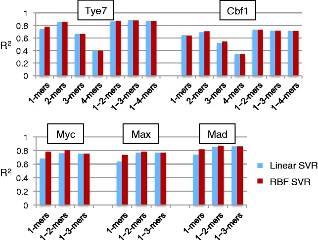
Table 2 reports the numbers of features that were selected for each feature set and TF. These numbers are small such that our models become interpretable, a desirable property for understanding how binding is enacted. This algorithm also provides a short list of features and their importance scores that reflect how often each feature was selected. To determine whether a particular sequence feature has a positive or negative influence on TF binding, we can look at the sign of the feature weight calculated from the linear SVR model (Section 3.4). As an example, Figure 8 shows the selected features for Cbf1 and Tye7, ordered by position on the flank from the core to the extremity (see Fig. 3), and then by k-mer size (i.e. first 1-mers and then 2-mers). The second-to-last column gives the importance score assigned to each feature by our algorithm, and the last column is the coefficient assigned to it when a linear SVR is trained on the selected set to predict binding intensity. We observe that the order on positions correlates well with the importance score order, suggesting that, as expected, positions right next to the E-box are more important than positions further away. Our selection procedure does identify features in the distal flanks that appear to be important for model accuracy (e.g. feature AA at position 11 in the Tye7 model, Fig. 8). Interestingly, the selected distal features are mostly 2-mers that exhibit specific DNA shape characteristics. For example, AA/AT dimers are typically bent toward the minor groove, and AA/TT shows the largest roll among all dimers (Zhurkin et al., 1991). Both minor groove width and roll are important for DNA binding by TFs (Gordân et al., 2013; Rohs et al., 2010).

Table 2.

Size of feature set selected by the Stable LASSO algorithm

Feature set	Cbf1	Tye7	Mad	Max	Myc
1–2-mers	20	20	35	25	22
1–3-mers	56	46	130	98	95

Fig. 8.

Selected features for Cbf1 (top) and Tye7 (bottom) ordered by position on the flank and length. Positions are specified relative to the core of the binding site (position 1 is the closest to the core). The second-to-last column is the area importance score of the feature, and the last column reports the weight coefficient attributed to the feature by a linear SVR. In red, we show the features with the six top coefficients; the blue features are those that contribute negatively to binding

4.4 Model specificity

When trying to predict TF–DNA interactions using models of DNA binding specificity, a difficult problem arises in the case of paralogous TFs (i.e. TFs that belong to the same protein family). Such TFs often have highly similar DNA binding specificities (Badis et al., 2009; Jolma et al., 2013), despite the fact that they are observed to interact with different sets of genomic sites in vivo (ENCODE Project Consortium, 2012). For some paralogous TFs, simple models such as PWMs are sufficient to capture differences in sequence preferences (Fong et al., 2012; Zhou and O’Shea, 2011). In many cases, however, the PWMs of paralogous TFs are virtually identical. Two such examples are studied in this article: Saccharomyces cerevisiae TFs Cbf1 and Tye7, and Homo sapiens TFs Myc, Max and Mad.

Cbf1 and Tye7 bind distinct sets of targets sites in yeast cells and have different regulatory functions (Harbison et al., 2004; Kent et al., 2004; Nishi et al., 1995). However, their PWMs are similar (MacIsaac et al., 2006; Zhu et al., 2009) (Fig. 1A) and cannot be used to distinguish the genomic regions bound in vivo by the two TFs with any specificity (Gordân et al., 2013). Myc, Max and Mad are members of a network of TFs that controls cell proliferation, differentiation and death. Despite playing different roles in the cell and having different sets of targets sites in vivo (ENCODE Project Consortium, 2012), Myc, Max and Mad have almost identical PWMs (Fig. 1B). Myc, Max and Mad PWMs cannot be used to differentiate between the genomic regions bound in vivo by these factors (Munteanu and Gordân, 2013).

To illustrate that our regression-based approach can generate TF–DNA binding models specific enough to distinguish between paralogous TFs, we performed a comparison among three different types of models: (i) available PWMs of size 10 for the TFs of interest (Munteanu and Gordân, 2013; Zhu et al., 2009); (ii) linear SVR models trained on custom PBM data using 1-mer features from the core 10 positions (these models are technically equivalent to PWMs of size 10, but learned from our quantitative PBM data); and (iii) RBF SVR models trained on custom PBM data following feature selection. We trained each model on data for one TF and used it to predict the binding specificity of related TFs. All the PWMs used in this analysis have been derived from universal PBM data and are in good agreement with previously reported motifs for the same TFs (Munteanu and Gordân, 2013; Zhu et al., 2009). We chose PWMs of size 10 because they obtained the best correlation coefficients between the PWM log ratio scores (for the putative binding site in each PBM probe) and the PBM log signal intensity.

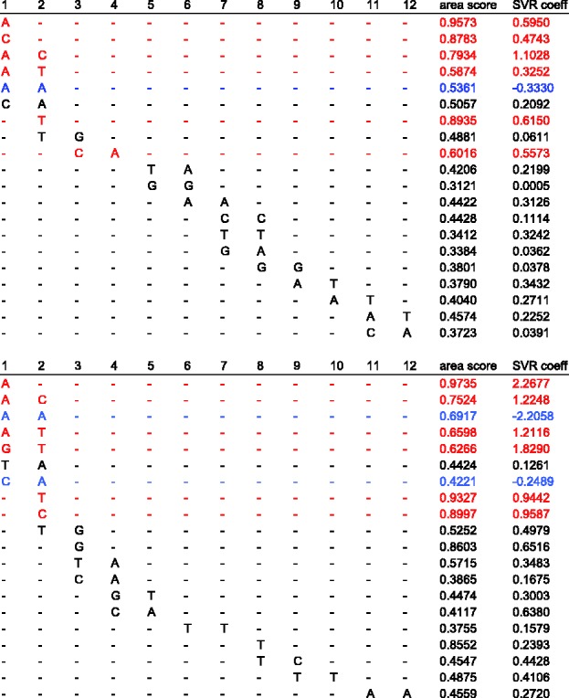
Figures 9 and 10 present the results of our specificity analysis, reporting the squared correlation coefficients between predicted and true binding intensities. In general, we notice that a model learned on TF A is less accurate at predict intensity for TF B than the model actually trained on data for TF B. For instance, our best SVR models after stability selection for yeast TFs were obtained on 1–2-mer features. In a 10-fold cross-validation test, the model trained on Cbf1 data proved highly accurate at predicting Cbf1 binding specificity (R² = 0.737) and not so accurate at predicting Tye7 specificity (R² = 0.461); similarly for Tye7 (Figs 9 and 10A).

Fig. 9.

Scatter plots of predicted versus true DNA binding specificity for regression-based models learned on the yeast data, using prior stability selection on 1–2-mer features. The ‘predicted binding specificity’ values represent predicted PBM log intensities. The ‘true binding specificity values’ represent actual PBM log intensities. Top panels: predicting DNA binding specificity for Cbf1 from a model learned on Cbf1 data (left) and Tye7 data (right). Bottom panels: predicting DNA binding specificity for Tye7 from a model learned on Cbf1 data (left) and Tye7 data (right). All tests were done using 10-fold cross-validation

Fig. 10.

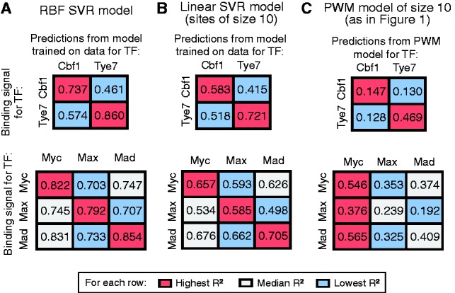
The specificity of RBF regression models with feature selection (using 1–2-mers for Cbf1/Tye7 and 1–3-mers for Myc/Max/Mad) (A), linear SVR 1-mers models trained on sites of size 10 (B) and PWM models of size 10 (C) was tested by comparing performance when predicting the binding intensity of test sequences from a model trained on the same TF versus a different TF. Numbers represent R² values

The two PWM models in our comparison (Fig. 10B and C) exhibit smaller and more similar correlation coefficients, and are therefore less accurate and less specific. For instance, we see that predicting binding signal for Cbf1 from the Cbf1 versus the Tye7 PWMs gives similar results (Fig. 10C) (R² = 0.147 and 0.130, respectively). Learning PWM-like models from the custom PBM data improves both the accuracy and the specificity of the models (Fig. 10B), but the best models are the ones that include non-independent contributions and are trained on custom PBM data (Fig. 10A). These results suggest that highly quantitative data (such as the custom PBM data in our study) allow us to gain both in specificity and accuracy. In addition, departing from the standard PWM model (by adding dependencies between adjacent positions and non-linear contributions to binding) helps improve the models even further on both levels.

5 DISCUSSION

We have presented a new approach for learning regression-based models of protein–DNA binding specificity from quantitative TF binding data, using SVR with feature selection. When tested on yeast and human TF binding data, our models are able to predict the specificity of each TF of interest. In addition, we show that the regression models trained on custom PBM data are able to distinguish binding behaviors of paralogous TFs, even when their PWM models are similar. Several factors contribute to the accuracy and specificity of our TF–DNA binding models.

First, we train our regression models on quantitative high-resolution data obtained using a high-throughput in vitro technology (PBM). This allows us to train complex models of specificity without the risk of overfitting the training data. High-throughput, in vitro data, including data generated using the PBM technology, has been previously used to train complex models of TF–DNA binding specificity (Agius et al., 2010; Annala et al., 2011; Weirauch et al., 2013). Our approach is somewhat similar to the work of Agius et al. (2010) and Annala et al. (2011), who also learn regression models from PBM data. However, both these studies use PBM data generated using universal array designs, which contain artificial DNA sequences designed to collectively cover all possible 10-mers (Berger et al., 2006). When using such an array design, each probe on the array may contain 0, 1 or more binding sites for the TF of interest, and these binding sites may be located at any position along the probe (i.e. any position relative to the free DNA end). Given the well-characterized positional bias in the universal PBM data (Berger et al., 2006), models trained on these data either try to learn the bias (Zhao and Stormo, 2011) or implicitly assume that the bias will average out when multiple probes are considered (Annala et al., 2011; Weirauch et al., 2013). In contrast, our custom microarray is designed so that each probe contains a single putative binding site located at the same location related to the free DNA end. This allows us to learn regression models that take into account k-mer occurrences at specific positions relative to the core of the binding site, as opposed to k-mers occurrences along the probes as done previously in Annala et al. (2011). The use of positional information makes our models easier to interpret than simple k-mer based models.

Second, by using a feature selection procedure, we restrict our regression models to a small number of parameters while maintaining a high prediction accuracy. This makes our models easier to visualize and interpret than other complex models of DNA binding specificity. For example, Agius et al. (2010) have also developed SVR-based models trained on PBM data. Their models fit the universal PBM data very well; however, the models are based on a special string kernel that makes is difficult to identify specific features that are important for model accuracy. In contrast, our feature selection procedure identifies relevant sequence features and also reports how frequently each feature is selected and how it contributes to the binding affinity (see Fig. 8).

Third, unlike the widely used PWM models, our regression models take into account non-independent contribution from individual bases in a TF binding site, by using the RBF kernel in the SVR algorithm and by incorporating 2-mer and 3-mer features. Importantly, our algorithm selects sequence features not only in the regions next to the CACGTG core but also in distal flanking regions, where the TF might not make specific DNA contacts. This suggests that the flanking regions may have an indirect influence on the binding affinity, possibly exerted through DNA shape, a hypothesis that we have tested previously for yeast TFs Cbf1 and Tye7 (Gordân et al., 2013). We note, however, that the current study is different from our previous work in several respects: previously, we neither performed any feature selection nor tried to interpret the specificity models; instead, we focused on the importance of intrinsic sequence preferences of paralogous TFs Cbf1 and Tye7 for achieving in vivo specificity, and on the potential role of DNA shape in providing a mechanistic explanation for the influence of flanking regions on DNA binding affinity. In the current study, we generate custom data for human TFs in addition to using the yeast data from Gordân et al. (2013), and we focus on using feature selection to get more accurate and interpretable models of binding specificity.

Future work will include developing similar models for TFs from other structural classes and organisms, as well as refining the feature selection procedure and testing other feature selection methods (Maldonado and Weber, 2010; Nguyen and de la Torre, 2010; Yang and Ong, 2010) that might help us identify sequence features relevant for model accuracy.

In conclusion, our regression-based approach for learning complex models of TF–DNA binding specificity from custom PBM data can be easily extended and improved, and we anticipate that the proposed regression models will help explain, at least in part, how paralogous TFs with highly similar PWMs are able to interact with distinct genomic targets.

REFERENCES

- Agius P, et al. High resolution models of transcription factor-DNA affinities improve in vitro and in vivo binding predictions. PLoS Comput. Biol. 2010;6:e1000916. doi: 10.1371/journal.pcbi.1000916. [DOI] [PMC free article] [PubMed] [Google Scholar]
- Annala M, et al. A linear model for transcription factor binding affinity prediction in protein binding microarrays. PLoS One. 2011;6:e20059. doi: 10.1371/journal.pone.0020059. [DOI] [PMC free article] [PubMed] [Google Scholar]
- Bach FR. 2008. Bolasso: Model consistent LASSO estimation through the bootstrap. In: Cohen,W.W., McCallum,A. and Roweis,S.T. (eds.) Proceedings of the 25th International Conference on Machine Learning, New York, NY, USA. [Google Scholar]
- Badis G, et al. Diversity and complexity in DNA recognition by transcription factors. Science. 2009;324:1720–1723. doi: 10.1126/science.1162327. [DOI] [PMC free article] [PubMed] [Google Scholar]
- Barash Y, et al. 2003. Modeling dependencies in protein-DNA binding sites. In: Proceedings of RECOMB 2003. New York, NY, USA, pp. 28–37. [Google Scholar]
- Benos P, et al. Additivity in protein-DNA interactions: how good an approximation is it? Nucleic Acids Res. 2002;30:4442–4451. doi: 10.1093/nar/gkf578. [DOI] [PMC free article] [PubMed] [Google Scholar]
- Berger M, et al. Compact, universal DNA microarrays to comprehensively determine transcription-factor binding site specificities. Nat. Biotechnol. 2006;24:1429–1435. doi: 10.1038/nbt1246. [DOI] [PMC free article] [PubMed] [Google Scholar]
- Berger MF, Bulyk ML. Universal protein-binding microarrays for the comprehensive characterization of the DNA binding specificities of transcription factors. Nat. Protoc. 2009;4:393–411. doi: 10.1038/nprot.2008.195. [DOI] [PMC free article] [PubMed] [Google Scholar]
- Bulyk ML, et al. Nucleotides of transcription factor binding sites exert interdependent effects on the binding affinities of transcription factors. Nucleic Acids Res. 2002;30:1255–1261. doi: 10.1093/nar/30.5.1255. [DOI] [PMC free article] [PubMed] [Google Scholar]
- Efron B, et al. Least angle regression. Ann. Stat. 2004;32:407–499. [Google Scholar]
- ENCODE Project Consortium. An integrated encyclopedia of DNA elements in the human genome. Nature. 2012;489:57–74. doi: 10.1038/nature11247. [DOI] [PMC free article] [PubMed] [Google Scholar]
- Fong AP, et al. Genetic and epigenetic determinants of neurogenesis and myogenesis. Dev. Cell. 2012;22:721–735. doi: 10.1016/j.devcel.2012.01.015. [DOI] [PMC free article] [PubMed] [Google Scholar]
- Gordân R, et al. Distinguishing direct versus indirect transcription factor-DNA interactions. Genome Res. 2009;19:2090–2100. doi: 10.1101/gr.094144.109. [DOI] [PMC free article] [PubMed] [Google Scholar]
- Gordân R, et al. Curated collection of yeast transcription factor DNA binding specificity data reveals novel structural and gene regulatory insights. Genome Biol. 2011;12:R125. doi: 10.1186/gb-2011-12-12-r125. [DOI] [PMC free article] [PubMed] [Google Scholar]
- Gordân R, et al. Genomic regions flanking E-box binding sites influence DNA binding specificity of bHLH transcription factors through DNA shape. Cell Rep. 2013;3:1093–1104. doi: 10.1016/j.celrep.2013.03.014. [DOI] [PMC free article] [PubMed] [Google Scholar]
- Harbison C, et al. Transcriptional regulatory code of a eukaryotic genome. Nature. 2004;431:99–104. doi: 10.1038/nature02800. [DOI] [PMC free article] [PubMed] [Google Scholar]
- Haury AC, et al. TIGRESS: Trustful inference of gene regulation using stability selection. BMC Syst. Biol. 2012;6:145. doi: 10.1186/1752-0509-6-145. [DOI] [PMC free article] [PubMed] [Google Scholar]
- Jauch R, et al. The crystal structure of the Sox4 HMG domain-DNA complex suggests a mechanism for positional interdependence in DNA recognition. Biochem. J. 2012;443:39–47. doi: 10.1042/BJ20111768. [DOI] [PubMed] [Google Scholar]
- Jolma A, et al. Multiplexed massively parallel SELEX for characterization of human transcription factor binding specificities. Genome Res. 2010;20:861–873. doi: 10.1101/gr.100552.109. [DOI] [PMC free article] [PubMed] [Google Scholar]
- Jolma A, et al. DNA binding specificities of human transcription factors. Cell. 2013;152:327–339. doi: 10.1016/j.cell.2012.12.009. [DOI] [PubMed] [Google Scholar]
- Kaplan T, et al. Quantitative models of the mechanisms that control genome-wide patterns of transcription factor binding during early Drosophila development. PLoS Genet. 2011;7:e1001290. doi: 10.1371/journal.pgen.1001290. [DOI] [PMC free article] [PubMed] [Google Scholar]
- Kent NA, et al. Cbf1p is required for chromatin remodeling at promoter-proximal CACGTG motifs in yeast. J. Biol. Chem. 2004;279:27116–27123. doi: 10.1074/jbc.M403818200. [DOI] [PubMed] [Google Scholar]
- Lin CY, et al. Transcriptional amplification in tumor cells with elevated c-Myc. Cell. 2012;151:56–67. doi: 10.1016/j.cell.2012.08.026. [DOI] [PMC free article] [PubMed] [Google Scholar]
- MacIsaac KD, et al. An improved map of conserved regulatory sites for Saccharomyces cerevisiae. BMC Bioinformatics. 2006;7:113. doi: 10.1186/1471-2105-7-113. [DOI] [PMC free article] [PubMed] [Google Scholar]
- Maerkl SJ, Quake SR. A systems approach to measuring the binding energy landscapes of transcription factors. Science. 2007;315:233–237. doi: 10.1126/science.1131007. [DOI] [PubMed] [Google Scholar]
- Maldonado S, Weber R. IJCNN 2010. Barcelona, Spain: 2010. Feature selection for support vector regression via kernel penalization; pp. 1–7. [Google Scholar]
- Man TK, Stormo GD. Non-independence of Mnt repressor-operator interaction determined by a new quantitative multiple fluorescence relative affinity (QuMFRA) assay. Nucleic Acids Res. 2001;29:2471–2478. doi: 10.1093/nar/29.12.2471. [DOI] [PMC free article] [PubMed] [Google Scholar]
- Meinshausen N, Bühlmann P. Stability selection. J. R. Stat. Soc. Ser. B. 2010;72:417–473. [Google Scholar]
- Munteanu A, Gordân R. Distinguishing between genomic regions bound by paralogous transcription factors. Recomb2013. Lect. Notes Comp. Sci. 2013;7821:145. [Google Scholar]
- Nguyen MH, de la Torre F. Optimal feature selection for support vector machines. Pattern Recogn. 2010;43:584–591. [Google Scholar]
- Nishi K, et al. The GCR1 requirement for yeast glycolytic gene expression is suppressed by dominant mutations in the SGC1 gene, which encodes a novel basic-helix-loop-helix protein. Mol. Cell. Biol. 1995;15:2646–2653. doi: 10.1128/mcb.15.5.2646. [DOI] [PMC free article] [PubMed] [Google Scholar]
- Pique-Regi R, et al. Accurate inference of transcription factor binding from DNA sequence and chromatin accessibility data. Genome Res. 2011;21:447–455. doi: 10.1101/gr.112623.110. [DOI] [PMC free article] [PubMed] [Google Scholar]
- Rohs R, et al. Origins of specificity in protein-DNA recognition. Annu. Rev. Biochem. 2010;79:233–269. doi: 10.1146/annurev-biochem-060408-091030. [DOI] [PMC free article] [PubMed] [Google Scholar]
- Sharon E, et al. A feature-based approach to modeling protein-DNA interactions. PLoS Comput. Biol. 2008;4:e1000154. doi: 10.1371/journal.pcbi.1000154. [DOI] [PMC free article] [PubMed] [Google Scholar]
- Siddharthan R. Dinucleotide weight matrices for predicting transcription factor binding sites: generalizing the position weight matrix. PLoS One. 2010;5:e9722. doi: 10.1371/journal.pone.0009722. [DOI] [PMC free article] [PubMed] [Google Scholar]
- Smola AJ, Schölkopf B. A tutorial on support vector regression. Stat. Comput. 2004;14:199–222. [Google Scholar]
- Staden R. Computer methods to locate signals in nucleic acid sequences. Nucleic Acids Res. 1984;12(1 Pt 2):505–519. doi: 10.1093/nar/12.1part2.505. [DOI] [PMC free article] [PubMed] [Google Scholar]
- Stormo GD. DNA binding sites: representation and discovery. Bioinformatics. 2000;16:16–23. doi: 10.1093/bioinformatics/16.1.16. [DOI] [PubMed] [Google Scholar]
- Tibshirani R. Regression shrinkage and selection via the lasso. J. R. Stat. Soc. Ser. B. 1996;58:267–288. [Google Scholar]
- Tomovic A, Oakeley EJ. Position dependencies in transcription factor binding sites. Bioinformatics. 2007;23:933–941. doi: 10.1093/bioinformatics/btm055. [DOI] [PubMed] [Google Scholar]
- Vapnik VN. Statistical Learning Theory. New-York, NY: Wiley; 1998. [Google Scholar]
- Weirauch MT, et al. Evaluation of methods for modeling transcription-factor sequence specificity. Nat. Biotechnol. 2013;31:126–134. doi: 10.1038/nbt.2486. [DOI] [PMC free article] [PubMed] [Google Scholar]
- Workman CT, et al. enoLOGOS: a versatile web tool for energy normalized sequence logos. Nucleic Acids Res. 2005;33:W389–W392. doi: 10.1093/nar/gki439. [DOI] [PMC free article] [PubMed] [Google Scholar]
- Yang JB, Ong CJ. ACM SIGKDD. New York, NY, USA: ACM; 2010. Feature selection for support vector regression using probabilistic prediction; pp. 343–352. [Google Scholar]
- Zhao Y, Stormo GD. Quantitative analysis demonstrates most transcription factors require only simple models of specificity. Nat. Biotechnol. 2011;29:480–483. doi: 10.1038/nbt.1893. [DOI] [PMC free article] [PubMed] [Google Scholar]
- Zhao Y, et al. Inferring binding energies from selected binding sites. PLoS Comput. Biol. 2009;5:e1000590. doi: 10.1371/journal.pcbi.1000590. [DOI] [PMC free article] [PubMed] [Google Scholar]
- Zhao Y, et al. Improved models for transcription factor binding site identification using nonindependent interactions. Genetics. 2012;191:781–790. doi: 10.1534/genetics.112.138685. [DOI] [PMC free article] [PubMed] [Google Scholar]
- Zhou Q, Liu JS. Modeling within-motif dependence for transcription factor binding site predictions. Bioinformatics. 2004;20:909–916. doi: 10.1093/bioinformatics/bth006. [DOI] [PubMed] [Google Scholar]
- Zhou X, O’Shea EK. Integrated approaches reveal determinants of genome-wide binding and function of the transcription factor Pho4. Mol. Cell. 2011;42:826–836. doi: 10.1016/j.molcel.2011.05.025. [DOI] [PMC free article] [PubMed] [Google Scholar]
- Zhu C, et al. High-resolution DNA binding specificity analysis of yeast transcription factors. Genome Res. 2009;19:556–566. doi: 10.1101/gr.090233.108. [DOI] [PMC free article] [PubMed] [Google Scholar]
- Zhurkin VB, et al. Static and statistical bending of DNA evaluated by Monte Carlo simulations. Proc. Natl Acad. Sci. USA. 1991;88:7046–7050. doi: 10.1073/pnas.88.16.7046. [DOI] [PMC free article] [PubMed] [Google Scholar]