

Abstract
Motivation: Template-based modeling, including homology modeling and protein threading, is the most reliable method for protein 3D structure prediction. However, alignment errors and template selection are still the main bottleneck for current template-base modeling methods, especially when proteins under consideration are distantly related.
Results: We present a novel context-specific alignment potential for protein threading, including alignment and template selection. Our alignment potential measures the log-odds ratio of one alignment being generated from two related proteins to being generated from two unrelated proteins, by integrating both local and global context-specific information. The local alignment potential quantifies how well one sequence residue can be aligned to one template residue based on context-specific information of the residues. The global alignment potential quantifies how well two sequence residues can be placed into two template positions at a given distance, again based on context-specific information. By accounting for correlation among a variety of protein features and making use of context-specific information, our alignment potential is much more sensitive than the widely used context-independent or profile-based scoring function. Experimental results confirm that our method generates significantly better alignments and threading results than the best profile-based methods on several large benchmarks. Our method works particularly well for distantly related proteins or proteins with sparse sequence profiles because of the effective integration of context-specific, structure and global information.
Availability: http://raptorx.uchicago.edu/download/.
Contact: jinboxu@gmail.com
1 INTRODUCTION
Protein structure is essential for the understanding of protein functions. Predicting the 3D structure of a protein from its sequence remains one of the grand challenges confronting computational biologists. Template-based modeling (TBM), such as homology modeling and protein threading, is the most reliable method and can produce reasonable 3D models for about two-third of the proteins without solved structures. TBM is based on the observation that protein structures are much more conserved than sequences. That is, given a target protein sequence, we can predict its 3D structure by aligning it to structurally similar protein structures in PDB. The model quality of TBM depends on sequence-template alignment and template selection, both of which are challenging when only distantly related templates are available for a protein sequence under prediction.
The threading accuracy critically depends on the choice of a threading scoring function (Meng et al., 2011). Most of current methods make heavy use of position-specific information, such as sequence profile, which is usually represented as a position-specific scoring matrix or a profile HMM (Eddy, 1998; Eskin and Snir, 2007; Jaroszewski et al., 2005; Söding, 2005). Although sequence profile is effective on homolog detection, it is only position specific, but not context specific. Further, it is also lack of structure information (e.g. secondary structure and solvent accessibility). Context-specific information refers to the information in the sequential neighborhood of one residue. The neighboring residues of a given residue play an important role in shaping the mutation pattern of the residue. Few alignment methods, such as CS-BLAST (Biegert and Söding, 2009) are developed to make use of context-specific information. Even CS-BLAST makes use of only sequence, but not context-specific structure information. To the best of our knowledge, no protein threading method has integrated well both context-specific sequence and structure information.
Although many protein alignment methods use only local information, a few protein threading methods (Akutsu and Miyano, 1999; Godzik et al., 1992; Jones et al., 1992; Xu et al., 2003) were developed to use global information, such as pairwise contact potential, which quantifies how well two sequence residues can be placed into two template positions in a contact. However, the gain from pairwise contact potential is not significant as compared with the impact of sequence profile on protein alignments. The underlying reason may be that the contact-based pairwise potentials used in these threading methods do not carry too much extra signal. To significantly improve the effectiveness of global information especially pairwise potential in protein threading, this article studies a context-specific distance-based pairwise potential. Our pairwise potential is built on context-specific information and much more sensitive than the context-independent contact-based pairwise potentials and, thus, greatly helps improve protein threading.
This article presents a novel context-specific alignment potential for protein threading, including both alignment and template selection. Our alignment potential measures the log-odds ratio of one alignment being generated from two related proteins to being generated from two unrelated proteins, by integrating context-specific local and global information. An alignment is assumed to be optimal if it maximizes the alignment potential. The local alignment potential quantifies how well one sequence residue can be aligned to one template residue based on context-specific information of these two residues. The global alignment potential quantifies how well two sequence residues can be placed into two template positions at a given distance, again based on residue context-specific information.
In this article, the context of one residue includes a variety of correlated protein features, such as sequence (profile) information, (predicted) secondary structure and solvent accessibility, amino acid physic-chemical properties in a local window centered at the residue. We integrate these correlated protein features into an accurate alignment potential using advanced statistical learning methods, including conditional neural fields (Peng et al., 2009). Experimental results show that our context-specific alignment potential is much more sensitive than the widely used context-independent or profile-based (which is position specific) scoring function, generating significantly better alignments and threading results than the best profile-based methods on several large benchmarks. Our method works particularly well for distantly related proteins or proteins with sparse sequence profiles because of the effective integration of context-specific, structure and global information.
2 METHODS
2.1 Protein alignment potential
We represent one alignment A between two proteins as a sequence of alignment states  , where L is the alignment length and
  is the alignment state at position i. There are three possible alignment states M, It and Is, where M represents two residues being aligned, It denotes an insertion in the template and Is denotes an insertion in the sequence.
2.1.1 Definition of alignment potential
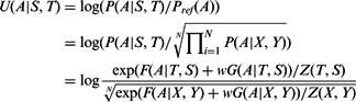
Similar to many amino acid substitution matrices, such as BLOSUM (Henikoff and Henikoff, 1992) and PAM (Dayhoff, 1978), which define the mutation potential of two amino acids, we define the potential of one protein alignment. Given a protein sequence S and a template T and one of their alignments A, let P(A|S, T) denote the probability of A being generated from S and T using our alignment method. We define the potential of A, denoted as U(A|S, T), as follows.
| (1) |
where  is the background (or reference) probability of A, i.e. the probability of A being generated from two randomly selected proteins with the same lengths as S and T, respectively. Intuitively, an alignment is good as long as its probability is much better than the expected probability. We assume that an alignment is optimal if it maximizes its potential. That is, given a sequence and a template, we can find their optimal alignment by maximizing the alignment potential function.
We use a recently developed probabilistic graphical model conditional neural fields (Peng et al., 2009) to calculate P(A|S, T) as follows (Ma et al., 2012),
| (2) |
where  is the model parameter vector to be trained, w (= 1.0) is a weight factor and
  is the normalization factor (i.e. partition function) summing over all possible alignments for a given protein pair. For the purpose of simplicity, we omit
  in the following sections unless we have to spell it out. The function F estimates the log-likelihood of one sequence residue being aligned to one template residue based on the input protein features. The function G estimates the log-likelihood of a pair of sequence residues being placed into two template positions at a given distance based on the input protein features. The functions F and G are called local and global alignment functions, respectively.
Once the forms of F(A|T, S) and G(A|T, S) are determined, we can train their parameters by maximum-likelihood. That is, given a set of training protein pairs and their reference alignments (built by a structure alignment tool), we maximize their occurring probability defined by Equation (2). However, as G(A|T, S) is a global alignment function, it is computationally hard to directly maximize Equation (2). In addition, it may cause overfitting by training the parameters of F and G simultaneously, as the parameter space is big. To avoid these problems, we determine the parameters of functions F and G separately, which will be explained in the following sections.
2.1.2 Reference state
We can calculate the reference alignment probability Pref(A) in Equation (1) by randomly sampling a set of protein pairs, each with the same lengths as the sequence S and template T, respectively, and then estimate the probability of alignment A based on these randomly sampled protein pairs. As long as we generate sufficient number of samplings, we shall be able to approximate  well. Here, we use the geometric mean to approximate the reference state as follows,
| (3) |
where N is the number of samplings and X and Y represent two sampled proteins with the same lengths as S and T, respectively. Combining Equation (1–3), the potential of one alignment A can be calculated as follows.
 |
(4) |
Note that an alignment is represented as a sequence of three states (match state M, insertion state at sequence Is and insertion state at template It), e.g. MMMMM IsIs MMMM It It It. Therefore, given two sequence–template pairs (S, T) and (X, Y), as long as S and T have the same lengths as X and Y, respectively, the alignment space (i.e. the set of all possible alignments) for S and T is the same as that for X and Y. That is, any S-to-T alignment is also a feasible alignment between X and Y, although it may have different probabilities. Conversely, any X-to-Y alignment is also a feasible alignment between S and T.
By definition, Z(S, T) is equal to the alignment space size times the mean value of the denominator in Equation (2). As S and T have the same alignment space as X and Y, Z(S, T) differs from Z(X, Y) only in the mean values of their corresponding denominators in Equation (2), which is independent of any specific alignment, but it may depend on protein residue composition. Therefore, we have,
| (5) |
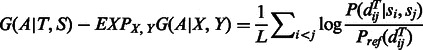
where EXP is the expectation operator, the first term of Equation (5) can be interpreted as local alignment potential and the second term can be interpreted as global alignment potential.
In Equation (5), c(S, T) depends on only the residue composition of S and T but not any specific alignment. In particular, c(S, T) is equal to 0 if the sampled protein pairs have similar residue composition as S and T. As such, for the purpose of finding the optimal alignment between S and T, we can simply ignore c(S, T). Therefore, the key challenge is to determine the local and global alignment potential functions in the right-hand side of Equation (5).
2.2 Local alignment potential
The function F in Equation (2) estimates the log-likelihood of one pair of residues being aligned based on their context-specific information. We represent an alignment A as a1, a2 , … , aL where L is the alignment length  and
and  are the alignment state at position i. As shown in Figure 1, we use a linear-chain context-specific conditional neural field to calculate F as follows.
| (6) |
where the function E is a neural network with one hidden layer, estimating the log-likelihood of state transition from  and
and  based on protein features in a local window (of size 11) centered at the two residues to be aligned. As in total there are nine possible state transitions in an alignment, we need nine different neural networks, each corresponding to one type of state transition.
Fig. 1.

Context-specific conditional neural fields for alignment. At each alignment position, the likelihood of state transition is calculated from context-specific information by a neural network. The hidden neurons non-linearly transform the input features
We use the maximum-likelihood method to train the parameters in function  . That is, given a set of reference alignments, we maximize their occurring probability defined later in the text.
| (7) |
where Z(T,S) is the partition function. This maximization problem can be solved using the L-BFGS (Liu and Nocedal, 1989) (i.e. limited-memory BFGS) algorithm, one of the quasi-Newton methods. Instead of exactly calculating the Hessian matrix required by the Newton’s method, BFGS approximates the inverse Hessian matrix to speed-up. We use a L2-norm regularization factor to restrict the search space of model parameters to avoid overfitting. The regularization factor is determined by 5-fold cross-validation.
Once the parameters of  are trained, the expectation term
  in Equation (5) can be calculated in advance by uniformly sampling a few thousand protein pairs. As the function
  depends on only a local window of protein features (i.e. independent of protein length), we do not need to calculate
  for each protein pair to be aligned, which saves a lot of computational time.
2.2.1 Protein features
The features we use for  include sequence similarity measured by BLOSUM (Henikoff and Henikoff, 1992), profile similarity, structure-derived amino acid substitution matrix (Tan et al., 2006), statistical potential-derived amino acid similarity matrix (Prlić et al., 2000), three-class and eight-class secondary structure similarity and three-state solvent accessibility similarity. The secondary structure and solvent accessibility of a template protein is calculated by DSSP (Kabsch and Sander, 1983). We predict the three-class and eight-class secondary structure types of a target protein using PSIPRED (McGuffin et al., 2000) and our in-house tool RaptorX-SS8 (Wang et al., 2011), respectively. We predict solvent accessibility of a target protein using our in-house tool. For each residue, we use all these features in a local window of size 11. In addition, all the similarity scores are computed as potentials. For example, let ssi and ssj denote the secondary structure types at sequence position i and template position j, respectively. The secondary structure similarity score for these two positions is calculated as log(P(ssi, ssj)/P(ssi) P(ssj)).
We do not use an affine gap penalty. Instead we use context-specific gap penalty depending on the following features: sequence profile, amino acid identity, hydropathy index, both three-class and eight-class secondary structure and three-state solvent accessibility. For disordered regions, no structure information is used.
2.3 Global alignment potential
The function G estimates the log-likelihood of a pair of sequence residues being placed to two template positions at a given distance. Instead of using a contact-based pairwise potential, here, we use a distance-based pairwise potential. We calculate the log-likelihood function G(A|T, S) as  and the expectation item in Equation (5)
 as
as  where i and j are two aligned positions,
  is the
  distance of the template residues at these two aligned positions,
  is the probability of two sequence residues si and sj being placed to two template positions at distance
  and
and  is the background probability of
  , which can be calculated by simple statistics. Therefore, the pairwise alignment potential is calculated as follows,
 |
(8) |
where L is the alignment length. As there are O(L2) pairwise terms in right-hand side of Equation (8), we normalize it by L so that the global alignment potential has the same scale as the local alignment potential.
To calculate  in Equation (8), we use the following equation,
| (9) |
where  represents the distance of the two sequence residues at the two aligned positions,
  is the conditional probability of
  on
on  and
and  is the conditional probability of the distance on the template estimated from the contexts (denoted
  and
and  ) of the two sequence residues. The intuition underlying Equation (8) is that if the alignment is good, the distance of a sequence residue pair shall match well with that of their aligned template residue pair. The conditional probability of Equation (9) can be calculated as
  using the chain rule. Where
  is the background probability, and
  is the joint probability of the pairwise distances of two aligned residue pairs and can be calculated by simple statistics using a set of non-redundant protein structure alignments generated by our in-house tool DeepAlign (Wang et al., 2013). As the distance between two sequence residues is unknown, we predict
  using a probabilistic neural network (PNN) implemented in our context-specific distance-dependent statistical potential package EPAD (Zhao and Xu, 2012). EPAD takes as input the contexts of two sequence residues and yields their distance probability distribution. The context of one residue includes sequence profile, predicted secondary structure and amino acid chemical properties in a local window centered at this residue.
Unlike previous threading methods that make use of contact-based pairwise potentials (Alexandrov et al., 1996; Lathrop and Smith, 1996; Miyazawa and Jernigan, 1996; Xu et al., 2003), we use a context-specific distance-based pairwise potential. Our pairwise potential is distance based and makes use of context-specific information; therefore, it is much more accurate than the context-independent contact-based potentials. The EPAD package was implemented before CASP10 started and has been blindly tested in CASP10 for template free modeling. The CASP10 results show that EPAD can successfully fold some targets with unusual fold (according to the CASP10 Free Modeling assessor Dr B. K. Lee). Our large-scale experimental test also indicates EPAD is much better than those context-independent distance-based pairwise potentials, such as DOPE (Shen and Sali, 2009), DFIRE (Zhou and Zhou, 2009) and RW (Zhang and Zhang, 2010) in ranking protein alignments (or template-based models) generated by both threading and structure alignment tools (Zhao and Xu, 2012).
3 RESULTS
Training and validation data: We constructed the training and validation data from BC40, a subset of PDB, in which any two proteins share <40% sequence identity. In total, we use a set of 1800 protein pairs as the training data, which covers most of the folds in the SCOP database, and a set of 500 protein pairs as the validation data. There is no redundancy between the training and validation data (i.e. <40% sequence identity). The training and validation data have the following properties: (i) all the proteins have lengths <400 and contain <10% of residues with missing coordinates; (ii) the TM-score (Zhang and Skolnick, 2005) of a protein pair is uniformly distributed from 0.55 to 1; and (iii) we use our in-house structure alignment tool DeepAlign (Wang et al., 2013) to generate the reference alignment for a protein pair. Each alignment has fewer than 50 middle gaps, and the number of terminal gaps is <20% of the alignment length.
Test data for alignment: We use the following three datasets to test the alignment accuracy of our method.
Set6K: a set of ∼6000 protein pairs. Any two target proteins in this set share <40% sequence identity. The TM-score of a protein pair is uniformly distributed between 0.55 and 0.8. Two proteins in a pair have small length difference. The protein pairs in Set6K have 5% of overlap with our training and validation data. By ‘overlap’ we mean that the proteins in one pair have sequence identity 30–50% with those in another pair.
Set4K: a set of 4547 protein pairs. Any two target proteins in the set share <25% sequence identity. The protein pairs in Set4K have 3% of overlap with our training and validation data. Two proteins in a pair have length difference >30%; therefore, this set can be used to test whether the domain boundary is correctly aligned.
Set180K: a very large set of 179 390 protein pairs. Any two proteins in most pairs share <40% sequence identity. The TM-score of a protein pair is uniformly distributed between 0 and 1. Note that the size of our training set is only 1% of this large set; therefore, the test result on this set is unlikely biased by the training set.
Test data for threading: We use the following two datasets to test the threading accuracy of our method.
Set 1000 × 6000: a large set constructed from PDB25, which consists of ∼6000 proteins. All the proteins in PDB25 are used as templates, and 1000 of them are randomly chosen as the target proteins. We predict the 3D structure for all the 1000 targets using the ∼6000 templates, but excluding self-threading.
CASP10: a set of 123 test proteins. We use the CASP official domain boundary definition for each test protein.
Evaluation criteria and programs to compare: We evaluate our threading method using both reference-dependent and reference-independent alignment accuracy. The reference-dependent accuracy is defined as the percentage of correctly aligned positions judged by the reference alignments, which are built using our in-house tool DeepAlign (Wang et al., 2013). We also built the reference alignments using other structure alignment tools, such as DALI, Matt and TMalign (Holm and Sander, 1993; Menke et al., 2008; Zhang and Skolnick, 2005) and observed similar performance trend. To evaluate the reference-independent alignment accuracy, we build a 3D model for the target protein using MODELLER (Šali et al., 2004) from its alignment to the template and then evaluate the quality of the resultant 3D model using TM-score. TM-score ranges from 0 to 1, indicating the worst and best model quality, respectively. As our ultimate goal is to predict 3D structure for a target protein, reference-independent alignment accuracy is more important than reference-dependent accuracy. We compare our method with the top-notch profile-based method HHalign, which is run with the option ‘-mact 0.1’.
As shown in Table 1, our method outperforms HHalign in terms of both reference-dependent and reference-independent alignment accuracy on the two benchmarks Set6K and Set4K. On these two sets, our method outperforms HHalign by 13.6 and 9%, respectively, in terms of the model quality (i.e. reference-independent accuracy). In terms of reference-dependent accuracy, our method is better than HHalign by only 8.8 and 5.2%, which is not as big as reference-independent accuracy. We also calculate the reference-dependent accuracy on Set6K and Set4K by allowing four-position off the exact match, as shown in Table 2, which indicates that our method is still much better than HHalign when four-position off the exact match is allowed.
Table 1.
Reference-dependent (Ref-dep) and reference-independent (Ref-ind) alignment accuracy on two benchmarks Set6K and Set4K
| Set6K |
Set4K |
|||
|---|---|---|---|---|
| Ref-dep (%) | Ref-indTM | Ref-dep (%) | Ref-indTM | |
| Our work | 52 | 0.52 | 63 | 0.62 |
| HHalign | 45 | 0.44 | 57 | 0.56 |
Note: Reference-independent alignment accuracy is measured by TM-score.
Table 2.
Reference-dependent alignment accuracy on two benchmarks of Set6K and Set4K
| Set6K |
Set4K |
|||
|---|---|---|---|---|
| Exact match (%) | Four-position off (%) | Exact match (%) | Four-position off (%) | |
| Our work | 52 | 57 | 63 | 67 |
| HHalign | 45 | 50 | 57 | 60 |
As shown in Table 3, on the very large Set180K set, our method yields slightly better performance than HHalign when two proteins under consideration are similar. This is not surprising, as most methods can generate pretty good alignments for two closely related proteins. When the TM-score of two proteins under consideration falls into [0.65, 0.80], our method outperforms HHalign by ∼3.3% in terms of the reference-dependent accuracy and by ∼7.6% in terms of the reference-independent accuracy. When the TM-score of two proteins under consideration falls into [0.40, 0.65], our method outperforms HHalign by ∼9.4% in terms of the reference-dependent accuracy and by ∼11.3% in terms of the reference-independent accuracy.
Table 3.
Reference-dependent (Ref-dep) and reference-independent (Ref-ind) alignment accuracy on the very large benchmark Set180K
| TM-score | Ref-dependent |
Ref-independentTM |
||
|---|---|---|---|---|
| HHalign (%) | Our work (%) | HHalign | Our work | |
| 0.80–1.00 | 83 | 84 | 0.78 | 0.79 |
| 0.65–0.80 | 60 | 62 | 0.52 | 0.56 |
| 0.40–0.65 | 32 | 35 | 0.30 | 0.34 |
| 0.25–0.40 | 11 | 19 | 0.16 | 0.20 |
Note: Reference-independent alignment accuracy is measured by TM-score. The protein pairs are divided into four groups depending on their structure similarity measured by TM-score.
When the TM-score of two proteins falls into [0.25, 0.40], our method outperforms HHalign by a very large margin in terms of reference-dependent alignment accuracy. However, in terms of the reference-independent alignment accuracy, the advantage of our method is not as big, although it is still substantial. This may be because that MODELLER cannot build a reasonable model from an alignment with too many errors. By the way, when the TM-score of two proteins is <0.4, it may not be so important to generate an accurate alignment for them, as the resultant 3D model has low quality and, thus, will not be useful.
Threading performance on a large test set: We test the threading performance of our method and HHpred on Set 1000 × 6000. We run both our method and HHpred to predict the 3D structure for each of the 1000 targets using the ∼6000 templates. HHpred is run with its ‘realign’ option. That is, HHpred first searches through the template database using local alignment and then re-aligns a target to the top templates using global alignment. By doing so, HHpred can improve its modeling accuracy a little bit over the default mode. To speed-up, our method first aligns a target to all the templates using only the local alignment potential and then ranks all the templates using both the local and global alignment potentials described in Section 2. After ranking, only the first-ranked templates are used to build a 3D model by MODELLER for each target.
As shown in Figure 2, our method is significantly better than HHpred when the targets are not so easy (i.e. the HHpred model has TM-score <0.7). On the 1000 targets, our method and HHpred obtain average TM-score 0.566 and 0.517, respectively. Our method outperforms HHpred no matter whether the target is easy or hard. If we exclude the 170 easy targets (i.e. either our model or HHpred model has TM-score >0.8) from consideration, the accumulative TM-score obtained by our method and HHpred is 0.524 and 0.451, respectively. That is, our method is ∼16.1% better than HHpred. Further, as indicated by the yellow lines in Figure 3, our method can generate models with TM-score >0.5 for many targets for which HHpred fails to generate a model with TM-score >0.5. We use TM-score = 0.5 as a cut-off because when a model has TM-score >0.5, its overall fold is basically correct.
Fig. 2.

The quality of the models by our method and HHpred for the 1000 targets randomly chosen from PDB25. Each point represents two models generated by our method (y-axis) and HHpred (x-axis), respectively
Fig. 3.

Distribution of the model quality difference, measured by TM-score. Each blue column shows the number of targets for which our method is better by a given margin. Each red column shows the number of targets for which HHpred is better by a given margin
As shown in Figure 3, our method generates models better than HHpred by at least 0.05 for 342 targets, whereas HHpred is better than our method by this margin for only 93 targets. Further, the number of targets for which our method generates models better than HHpred by at least 0.10 is 197, whereas HHpred is better than our method by this margin for only 49 targets. In summary, our method has a large advantage over HHpred on hard targets.
Threading performance on CASP10 data set: We further evaluate the threading performance of our method on the most recent CASP10 targets. We use the CASP official domain boundary definition for each target, and in total there are 123 test proteins. To make the test as fair as possible, both our method and HHpred used the same set of templates and the same protein sequence database (i.e. NR), which were constructed before CASP10 started.
As shown in Figure 4, similar to what we have observed on the large threading test set, our method significantly outperforms HHpred when the targets are not so easy. Our method generates a model with TM-score >0.5 for a few targets for which HHpred fails to generate a model with TM-score >0.5. On the whole test set, our method and HHpred obtain accumulative TM-score 77.52 and 70.65, respectively. If we exclude the ‘Server’ targets from consideration and only look at the more challenging ‘Human/Server’ targets. The average TM-score obtained by our method and HHpred is 0.63 and 0.57, respectively. That is, our method is ∼10.5% better than HHpred.
Fig. 4.

The model quality, measured by TM-score, of our method and HHpred for the 123 CASP10 targets. Each point represents two models generated by our method (y-axis) and HHpred (x-axis), respectively
It is challenging to fairly compare our single-template threading method with the CASP10-participarting servers because that most of the CASP10 servers used a hybrid method instead of an individual threading method. For example, the first-ranked Zhang-Server integrated both consensus analysis of ∼10 individual threading programs and fragment-based 3D model building technique. The top-ranked HHpred server integrated new profile generation method, multi-template alignment and a better 3D model building technique. The top-ranked Robetta server used consensus results from three programs, including HHpred, RaptorX and SPARKS and also a new 3D model building method. Our RaptorX server, which is ranked No. 2 overall, used multiple-template threading, which can generate better 3D models than single-template threading for many targets especially the easy ones. In summary, the accumulative TM-score obtained by our single-template threading method described in this article is only 0.85 less than what was obtained by RaptorX in CASP10. It can be ranked No. 6 among all the CASP10-participating servers.
P-value: It is desirable that any structure prediction program can assign a confidence score to predicted models. Here, we use P-value to quantify the relative quality of the top-ranked templates and alignments. To calculate the P-value, we use a set of reference templates, which consist of ∼1800 single-domain templates with different SCOP folds. Given a target, we first thread it to this reference template database and then estimate an extreme value distribution from the ∼1800 alignment scores (i.e. alignment potentials). Based on this distribution, we calculate the P-value of each alignment when threading the target to the real template database. The P-value actually measures the quality of the template (and the alignment) by comparing it with the reference templates.
To measure the real model quality, we use both GDT (Global Distance Test) (Zemla et al., 1999) and uGDT (i.e. un-normalized GDT). GDT has been used as an official measure by CASP for many years. It measures the quality of a model by comparing it with the native and outputs a value from 0 to 100, indicating the worst and the best quality, respectively. uGDT is equal to GDT times the target length divided by 100. uGDT is more suitable when a large or multi-domain target protein can only be partially covered by good templates. In this case, GDT is likely to be small and not a good indicator even if the templates are closely related to the target, as GDT is normalized by the whole target length. However, uGDT is not good for a target with length smaller than 100. For example, when a target of 60 residues is covered by a template perfectly on 48 of the 60 residues, the uGDT of this alignment is 48, whereas the GDT is 80. In this case, GDT is more suitable than uGDT. In summary, we use max(uGDT,GDT) to measure the model quality. We say one alignment is reasonable when its resultant model has uGDT or GDT >50. We use 50 as a cut-off because that many proteins similar at only the fold level have GDT or uGDT ∼50.
As shown in Figure 5, the P-value is a reliable indicator of model quality. When P-value is small (i.e. <10−5), the models have uGDT or GDT ≥ 50. Even if P-value is <10−4, there are few models that have both uGDT and GDT < 50. That is, the prediction from our threading method is reliable when the P-value is <10−4.
Fig. 5.

The relationship between P-value and the model quality on the 123 CASP10 targets. The x-axis is the model quality measured by max(GDT, uGDT) and the y-axis is −log (P-value)
Contribution of the distance-based pairwise potential: To evaluate the contribution of our pairwise potential to alignment accuracy, we calculate the accuracy improvement resulting from adding our pairwise potential to the alignment potential using two benchmarks Set6K and Set4K. As shown in Table 4, our pairwise potential can improve reference-dependent accuracy by 3% and reference-independent accuracy by 0.01, respectively. We have not fully exploited the power of our pairwise alignment potential because it is computationally expensive. We just used our pairwise potential to refine the alignment generated by local alignment potential as follows. For each aligned position generated by our local potential, we allow it to move at most four positions to improve the total potential (i.e. local potential + pairwise potential). We expect that a more efficient pairwise potential optimization algorithm that can search a larger alignment space will further improve the alignment accuracy.
Table 4.
Contribution of pairwise potential to alignment accuracy, tested on two benchmarks Set6K and Set4K
| Set6K |
Set4K |
|||
|---|---|---|---|---|
| Ref-dep (%) | Ref-indTM | Ref-dep (%) | Ref-indTM | |
| Local potential | 49 | 0.51 | 60 | 0.61 |
| Local + pairwise | 52 | 0.52 | 63 | 0.62 |
Note: Reference-independent alignment accuracy is measured by TM-score.
We also evaluate the contribution of our pairwise potential to template selection. To speed-up, we generate alignments using our local alignment potential, and then rank all the templates using a linear combination of our local and pairwise alignment potentials (with equal weight). Experimental results on the 1000 × 6000 threading set and the CASP10 set indicate that the pairwise potential indeed improves template selection, as shown in Figures 6 and 7. On the 1000 × 6000 set, the average TM-score increases from 0.547 to 0.566 when the pairwise potential is used to rank the templates. On the CASP10 set, the accumulative TM-score increases from 75.58 to 77.52 when the pairwise potential is used. As shown in Figures 6 and 7, the context-specific pairwise potential is particularly helpful to hard targets.
Fig. 6.

Contribution of the distance-based pairwise alignment potential to Set 1000 × 6000. Each point represents the quality, measured by TM-score, of two models: one is generated using the local alignment potential only (x-axis), and the other using both the local and global alignment potentials (y-axis)
Fig. 7.

Contribution of the distance-based pairwise alignment potential to the CASP10 set. Each point represents the quality, measured by TM-score, of two models: one is generated using the local alignment potential only (x-axis), and the other using both the local and global alignment potentials (y-axis)
Case study: Here, we use two specific examples to further demonstrate the strength of our method. Both of these two cases are from our Set6K benchmark. The first example is to align two proteins 3qnrA and 2gffA, which have TMscore between 0.62 and 0.65 according to the structural alignments generated by TM-align (Zhang and Skolnick, 2005), Matt (Menke et al., 2008), Dali (Holm and Sander, 1993) and our in-house tool DeepAlign (Wang et al., 2013). That is, these two proteins are similar in structures but not much in sequences. Meanwhile, 2gffA contains two α and two β segments that are similar to one domain in 3qnrA. As shown in Figure 8, our method can correctly align >90% of the positions judged by the reference alignment (regardless of which structural alignment tools are used to generate it). In contrast, HHalign fails to align the second α and β segments. This is partially because HHalign favors generating short alignment. If we choose 3qnrA as the template to build a 3D model for 2gffA, the resultant models from our method and HHalign have TM-score 0.63 and 0.25, respectively.
Fig. 8.

Two alignments between 3qnrA and 2gffA generated by our method and HHalign. The blue and red colors demonstrate correctly aligned regions judged by the reference alignment. To save space, only one of the domains of 3qnrA is shown
We use another two proteins 3k53A and 1cb7A to showcase that our method and HHalign generate two alignments of nearly the same length, but our alignment has much better quality. As shown in Figure 9, our method aligns nearly 80% of positions correctly, whereas HHalign fails to align any position correctly. If we use 3k53A as the template to build models for 1cb7A, the resultant 3D models from our method and HHalign have TM-score 0.64 and 0.22, respectively. We can also examine the alignments visually. As shown in Figure 10A and B, our method aligns the local structure well, whereas HHalign seemingly produces a totally wrong alignment. In this case, both 3k53A and 1cb7A have pretty good sequence profile information, and the predicted secondary structure for 1cb7A is also accurate (>80%).
Fig. 9.

The alignments between 3k53A and 1cb7A generated by our method and HHalign. The blue and red colors indicate the correctly aligned regions
Fig. 10.

Superposition between proteins 3k53A and 1cb7A based on the alignments generated by our method and HHalign, respectively. The highlighted regions indicate the aligned residues
4 CONCLUSION
This article has presented a novel protein threading method using a context-specific alignment potential, which measures the log-odds ratio of one alignment being generated from two related proteins to being generated from two unrelated proteins. Intuitively, an alignment is regarded as good only when its estimated probability is much higher than the expected. Our alignment potential integrates both local and global context-specific and structure information through advanced machine learning techniques, such as conditional neural fields, which can combine a variety of highly correlated protein sequence and structure features, without worrying too much about overcounting and undercounting of features. Experimental results show that our context-specific alignment potential is much more sensitive than the widely used context-independent (e.g. profile-based) scoring function and yields significantly better alignments and threading results. Our method works particularly well for distantly related proteins or proteins with sparse sequence profiles because of the effective integration of context-specific, structure and global information.
This article also shows that our context-specific distance-based pairwise potential is helpful to protein threading, as opposed to the contact-based potentials previously used by some protein threading methods. Combined with our context-specific local alignment potential, our distance-based pairwise potential can help improve both alignment accuracy and template selection especially for hard targets. We expect that a more efficient algorithm that can optimize the pairwise potential better will yield more accurate alignments.
Acknowledgement
The authors are grateful to the University of Chicago Beagle team, TeraGrid and for their support of computational resources.
Funding: National Institutes of Health (R01GM0897532); National Science Foundation (DBI-0960390); NSF CAREER award CCF-1149811; Alfred P. Sloan Research Fellowship.
Conflict of Interest: none declared.
References
- Akutsu T, Miyano S. On the approximation of protein threading. Theor. Comput. Sci. 1999;210:261–275. [Google Scholar]
- Alexandrov NN, et al. Fast protein fold recognition via sequence to structure alignment and contact capacity potentials. Pac. Symp. Biocomput. 1996:53–72. [PubMed] [Google Scholar]
- Biegert A, Söding J. Sequence context-specific profiles for homology searching. Proc. Natl. Acad. Sci. USA. 2009;106:3770–3775. doi: 10.1073/pnas.0810767106. [DOI] [PMC free article] [PubMed] [Google Scholar]
- Dayhoff MO, et al. A model of evolutionary change in proteins. In: Dayhoff MO, editor. Atlas of Protein Sequence and Structure. 1978. Vol. 5, Supplement 3. NBRF, Washington, DC. pp. 345–358. [Google Scholar]
- Eddy SR. Profile hidden Markov models. Bioinformatics. 1998;14:755–763. doi: 10.1093/bioinformatics/14.9.755. [DOI] [PubMed] [Google Scholar]
- Eskin E, Snir S. Incorporating homologues into sequence embeddings for protein analysis. J. Bioinform. Comput. Biol. 2007;5:717–738. doi: 10.1142/s0219720007002734. [DOI] [PubMed] [Google Scholar]
- Godzik A, et al. Topology fingerprint approach to the inverse protein folding problem. J. Mol. Biol. 1992;227:227–238. doi: 10.1016/0022-2836(92)90693-e. [DOI] [PubMed] [Google Scholar]
- Henikoff S, Henikoff JG. Amino acid substitution matrices from protein blocks. Proc. Natl. Acad. Sci. USA. 1992;89:10915–10919. doi: 10.1073/pnas.89.22.10915. [DOI] [PMC free article] [PubMed] [Google Scholar]
- Holm L, Sander C. Protein structure comparison by alignment of distance matrices. J. Mol. Biol. 1993;233:123–138. doi: 10.1006/jmbi.1993.1489. [DOI] [PubMed] [Google Scholar]
- Jaroszewski L, et al. FFAS03: a server for profile–profile sequence alignments. Nucleic Acids Res. 2005;33:W284–W288. doi: 10.1093/nar/gki418. [DOI] [PMC free article] [PubMed] [Google Scholar]
- Jones DT, et al. A new approach to protein fold recognition. Nature. 1992;358:86–89. doi: 10.1038/358086a0. [DOI] [PubMed] [Google Scholar]
- Kabsch W, Sander C. Dictionary of protein secondary structure: pattern recognition of hydrogen-bonded and geometrical features. Biopolymers. 1983;22:2577–2637. doi: 10.1002/bip.360221211. [DOI] [PubMed] [Google Scholar]
- Lathrop RH, Smith TF. Global optimum protein threading with gapped alignment and empirical pair score functions. J. Mol. Biol. 1996;255:641–666. doi: 10.1006/jmbi.1996.0053. [DOI] [PubMed] [Google Scholar]
- Liu DC, Nocedal J. On the limited memory BFGS method for large scale optimization. Math. Program. 1989;45:503–528. [Google Scholar]
- Ma J, et al. A conditional neural fields model for protein threading. Bioinformatics. 2012;28:i59–i66. doi: 10.1093/bioinformatics/bts213. [DOI] [PMC free article] [PubMed] [Google Scholar]
- McGuffin LJ, et al. The PSIPRED protein structure prediction server. Bioinformatics. 2000;16:404–405. doi: 10.1093/bioinformatics/16.4.404. [DOI] [PubMed] [Google Scholar]
- Meng L, et al. Sequence alignment as hypothesis testing. J. Comput. Biol. 2011;18:677–691. doi: 10.1089/cmb.2010.0328. [DOI] [PMC free article] [PubMed] [Google Scholar]
- Menke M, et al. Matt: local flexibility aids protein multiple structure alignment. PLoS Comput. Biol. 2008;4:e10. doi: 10.1371/journal.pcbi.0040010. [DOI] [PMC free article] [PubMed] [Google Scholar]
- Miyazawa S, Jernigan RL. Residue-residue potentials with a favorable contact pair term and an unfavorable high packing density term, for simulation and threading. J. Mol. Biol. 1996;256:623–644. doi: 10.1006/jmbi.1996.0114. [DOI] [PubMed] [Google Scholar]
- Peng J, et al. Conditional neural fields. Adv. Neural Inf. Process. Syst. 2009;22:1419–1427. [Google Scholar]
- Prlić A, et al. Structure-derived substitution matrices for alignment of distantly related sequences. Protein Eng. 2000;13:545–550. doi: 10.1093/protein/13.8.545. [DOI] [PubMed] [Google Scholar]
- Šali A, et al. Evaluation of comparative protein modeling by MODELLER. Proteins. 2004;23:318–326. doi: 10.1002/prot.340230306. [DOI] [PubMed] [Google Scholar]
- Shen MY, Sali A. Statistical potential for assessment and prediction of protein structures. Protein Sci. 2009;15:2507–2524. doi: 10.1110/ps.062416606. [DOI] [PMC free article] [PubMed] [Google Scholar]
- Söding J. Protein homology detection by HMM–HMM comparison. Bioinformatics. 2005;21:951–960. doi: 10.1093/bioinformatics/bti125. [DOI] [PubMed] [Google Scholar]
- Tan YH, et al. Statistical potential-based amino acid similarity matrices for aligning distantly related protein sequences. Proteins. 2006;64:587–600. doi: 10.1002/prot.21020. [DOI] [PubMed] [Google Scholar]
- Wang Z, et al. Protein 8-class secondary structure prediction using conditional neural fields. Proteomics. 2011;11:3786–3792. doi: 10.1002/pmic.201100196. [DOI] [PMC free article] [PubMed] [Google Scholar]
- Wang S, et al. Protein structure alignment beyond spatial proximity. Scientific Reports. 2013;3:1448. doi: 10.1038/srep01448. [DOI] [PMC free article] [PubMed] [Google Scholar]
- Xu J, et al. RAPTOR: optimal protein threading by linear programming. J. Bioinform. Comput. Biol. 2003;1:95–117. doi: 10.1142/s0219720003000186. [DOI] [PubMed] [Google Scholar]
- Zemla A, et al. Processing and analysis of CASP3 protein structure predictions. Proteins. 1999;37:22–29. doi: 10.1002/(sici)1097-0134(1999)37:3+<22::aid-prot5>3.3.co;2-n. [DOI] [PubMed] [Google Scholar]
- Zhang Y, Skolnick J. TM-align: a protein structure alignment algorithm based on the TM-score. Nucleic Acids Res. 2005;33:2302–2309. doi: 10.1093/nar/gki524. [DOI] [PMC free article] [PubMed] [Google Scholar]
- Zhang J, Zhang Y. A novel side-chain orientation dependent potential derived from random-walk reference state for protein fold selection and structure prediction. PLoS One. 2010;5:e15386. doi: 10.1371/journal.pone.0015386. [DOI] [PMC free article] [PubMed] [Google Scholar]
- Zhao F, Xu J. A position-specific distance-dependent statistical potential for protein structure and functional study. Structure. 2012;20:1118–1126. doi: 10.1016/j.str.2012.04.003. [DOI] [PMC free article] [PubMed] [Google Scholar]
- Zhou H, Zhou Y. Distance-scaled, finite ideal-gas reference state improves structure-derived potentials of mean force for structure selection and stability prediction. Protein Sci. 2009;11:2714–2726. doi: 10.1110/ps.0217002. [DOI] [PMC free article] [PubMed] [Google Scholar]