

Abstract
Motivation: Protein contact map describes the pairwise spatial and functional relationship of residues in a protein and contains key information for protein 3D structure prediction. Although studied extensively, it remains challenging to predict contact map using only sequence information. Most existing methods predict the contact map matrix element-by-element, ignoring correlation among contacts and physical feasibility of the whole-contact map. A couple of recent methods predict contact map by using mutual information, taking into consideration contact correlation and enforcing a sparsity restraint, but these methods demand for a very large number of sequence homologs for the protein under consideration and the resultant contact map may be still physically infeasible.
Results: This article presents a novel method PhyCMAP for contact map prediction, integrating both evolutionary and physical restraints by machine learning and integer linear programming. The evolutionary restraints are much more informative than mutual information, and the physical restraints specify more concrete relationship among contacts than the sparsity restraint. As such, our method greatly reduces the solution space of the contact map matrix and, thus, significantly improves prediction accuracy. Experimental results confirm that PhyCMAP outperforms currently popular methods no matter how many sequence homologs are available for the protein under consideration.
Availability: http://raptorx.uchicago.edu.
Contact: jinboxu@gmail.com
1 INTRODUCTION
In this article, we say two residues of a protein are in contact if their Euclidean distance is <8 Å. The distance of two residues can be calculated using Cα or Cβ atoms, corresponding to Cα- or Cβ-based contacts. A protein contact map is a binary L × L matrix, where L is the protein length. In this matrix, an element with value 1 indicates the corresponding two residues are in contact; otherwise, they are not in contact. Protein contact map describes the pairwise spatial and functional relationship of residues in a protein. Predicting contact map using sequence information has been an active research topic in recent years partially because contact map is helpful for protein 3D structure prediction (Ortiz et al., 1999; Vassura et al., 2008; Vendruscolo et al., 1997; Wu et al., 2011) and protein model quality assessment (Zhou and Skolnick, 2007). Protein contact map has also been used to study protein structure alignment (Caprara et al., 2004; Wang et al., 2013; Xu et al., 2007).
Many machine-learning methods have been developed for protein contact prediction in the past decades (Fariselli and Casadio, 1999; Göbel et al., 2004; Olmea and Valencia, 1997; Punta and Rost, 2005; Vendruscolo and Domany, 1998; Vullo et al., 2006). For example, SVMSEQ (Wu and Zhang, 2008) uses support vector machines for contact prediction; NNcon (Tegge et al., 2009) uses a recursive neural network; SVMcon (Cheng and Baldi, 2007) also uses support vector machines plus features derived from sequence homologs; Distill (Baú et al., 2006) uses a 2D recursive neural network. Recently, CMAPpro (Di Lena et al., 2012) uses a multi-layer neural network. Although different, these methods are common in that they predict the contact map matrix element-by-element, ignoring the correlation among contacts and also physical feasibility of the whole-contact map (physical constraints are not totally independent of contact correlation). A special type of physical constraint is that a contact map matrix must be sparse, i.e. the number of contacts in a protein is only linear in its length.
Two recent methods [PSICOV (Jones et al., 2012) and Evfold (Morcos et al., 2011)] predict contacts by using only mutual information (MI) derived from sequence homologs and enforcing the aforementioned sparsity constraint. However, both of them demand for a large number (at least several hundreds) of sequence homologs for the protein under prediction. This makes the predicted contacts not useful in protein modeling, as a (globular) protein with many sequence homologs usually has similar templates in PDB; thus, template-based models are of good quality and hard to be further improved using predicted contacts. Conversely, a protein without close templates in PDB, which may require contact prediction, usually has few sequence homologs even if millions of protein sequences are now available. Further, these two methods enforce only a simple sparsity constraint (i.e. the total number of contacts in a protein is small), ignoring many more concrete constraints. To name a few, one residue can have only a small number of contacts, depending on its secondary structure and neighboring residues. The number of contacts between two β-strands is bounded by the strand length.
Astro-Fold (Klepeis and Floudas, 2003) possibly is the first method that applies physical constraints, which implicitly imply the sparsity constraint used by PSICOV and Evfold, to contact map prediction. However, some of the physical constraints are too restrictive and possibly unrealistic. For example, it requires that a residue in one β-strand can only be in contact with a residue in another β-strand. More importantly, Astro-Fold does not take into consideration evolutionary information; thus, it significantly reduces its prediction accuracy.
In this article, we present a novel method PhyCMAP for contact map prediction by integrating both evolutionary and physical constraints using machine learning [i.e. Random Forests (RF)] and integer linear programming (ILP). PhyCMAP first predicts the probability of any two residues forming a contact using evolutionary information (including MI), predicted secondary structure and distance-dependent statistical potential. PhyCMAP then infers a given number of top contacts based on predicted contact probabilities by enforcing a set of realistic physical constraints on the contact map. These restraints specify more concrete relationship among contacts and also imply the sparsity restraint used by PSICOV and Evfold. By combining both evolutionary and physical constraints, our method greatly reduces the solution space of contact map and leads to much better prediction accuracy. Experimental results confirm that PhyCMAP outperforms currently popular methods no matter how many sequence homologs are available for the protein under prediction.
2 METHODS
Overview. As shown in Figure 1, our method consists of several key components. First, we use RF to predict the contact probability of any two residues based on a few protein features related to these two residues. Then we use an ILP method to select a set of top contacts by maximizing their accumulative probabilities subject to a set of physical constraints. The resultant top contacts form a physically favorable contact map for the protein under consideration.
Fig. 1.
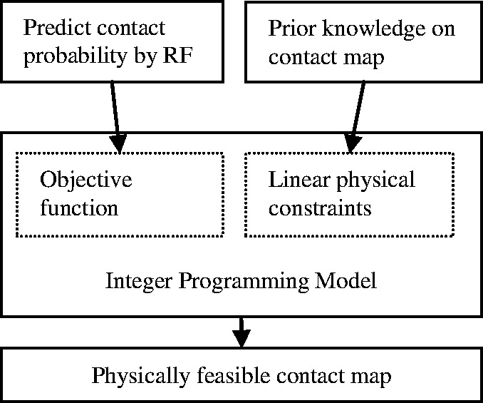
The overview of our approach
2.1 Predicting contact probability by Random Forests
We use RF to predict the probability of any two residues forming a contact using the following input features: EPAD (a context-specific distance-based statistical potential) (Zhao and Xu, 2012), PSIBLAST sequence profile (Altschul and Koonin, 1998), secondary structure predicted by PSIPRED (Jones, 1999), pairwise contact score and contrastive MI (CMI) derived from multiple sequence alignment (MSA) of the sequence homologs of the protein under prediction. The latter four features are calculated on the residues in a local window of size 5 centered at the residues under consideration. In total, there are ∼300 features for each residue pair. We trained our RF model using the Random Forest package in R (Breiman, 2001; Liaw and Wiener, 2002) and selected the model parameters by 5-fold cross-validation.
EPAD. The context-specific interaction potential of the Cα or Cβ atoms of two residues at all the possible distance bins is used as features. The atomic distance is discretized into some bins by 1 Å, and all the distance >15 Å is grouped into a single bin.
Sequence profile. The position-specific mutation scores at residues i and j and their neighboring residues are used.
In addition, a protein contact-based potential CCPC (Tan et al., 2006) and amino acid physic-chemical properties are also used as features of our RF model.
Homologous pairwise contact score (HPS). Let i and j denote two residues of the protein under consideration. Let H denote the set of all the sequence homologs. Given an MSA of all the homologs in H, we calculate the homologous pairwise contact score HPS for two residues  and
and  as follows.
where 
 denotes the residue in a homolog h aligned to residue i(j) in the query sequence.
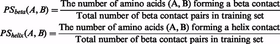
  is the probability of two amino acids
  forming a contact in a β-sheet.
  is the probability of two amino acids
  forming a contact connecting two helices. The probability is calculated as follows.
 |
The contrastive mutual information. Let mi,j denote the MI between these two residues i and j, which can be calculated from the MSA of all the sequence homologs. We define the CMI as the MI difference between one residue pair and all of its neighboring pairs, which can be calculated as follows.
The CMI measures how the co-mutation strength of one residue pair differs from its neighboring pairs. By using CMI instead of MI, we can remove the background bias of MI in a local region, as shown in Figure 2. In the case that there are only a small number of sequence homologs available, some conserved positions, which usually have entropy <0.3, may have very low MI, which may result in artificially high CMI. To avoid this, we directly set the CMI of these positions to 0.
Fig. 2.

The CMI (lower triangle) and MI (upper triangle) of protein 1j8bA.The native contact pairs are marked by boxes
2.2 The integer linear programming method
The variables. Let i and j denote residue positions and L the protein length. Let u and v index secondary structure segments of a protein. Let Begin(u) and End(u) denote the first and last residues of the segment u and SSeg(u) the set  . Let SStype(u) denote the secondary structure type of one residue or one segment u. Let Len(u) denote the length of the segment u. We use the binary variables in Table 1.
Table 1.
The binary variables used in the ILP formulation
| Variables | Explanations |
|---|---|
 |
Equal to 1 if there is a contact between two residues i and j. |
 |
Equal to 1 if two β-strands  and and  form an anti-parallel β-sheet. form an anti-parallel β-sheet. |
 |
Equal to 1 if two β-strands  and and  form a parallel β-sheet. form a parallel β-sheet. |
 |
Equal to 1 if two β-strands  and and  form a β-sheet. form a β-sheet. |
 |
Equal to 1 if there is an α-bridge between two helices  and and  . . |
 |
A non-negative integral relaxation variable of the  soft constraint. soft constraint. |
The objective function. Intuitively, we shall choose those contacts with the highest probability predicted by our RF model, i.e. the objective function shall be the sum of predicted probabilities of the selected contacts. However, the selected contacts shall also minimize the violation of the physical constraints. To enforce this, we use a vector of relaxation variables R to measure the degree to which all the soft constraints are violated. Thus, our objective function is as follows.
where  is the contact probability predicted by our RF model for two residues and
  is a linear penalty function where r runs over all the soft constraints. The relaxation variables will be further explained in the following section.
The constraints. We use both soft and hard constraints. There is a single relaxation variable for each group of soft constraint, but the hard constraints are strictly enforced. We penalize the violation of soft constraints by incorporating the relaxation variables to the objective function. The constraints in Groups 1, 2 and 6 are soft constraints. Those in Groups 3, 4, 5 and 7 are hard constraints, some of which are similar to what are used by Astro-Fold (Klepeis and Floudas, 2003).
Group 1. This group of soft constraints bound from above the total number of contacts that can be formed by a single residue  (in a secondary structure type
  ) with all the other residues in a secondary structure type
  .
.
where  is a constant empirically determined from our training data (Table 2), and
  is the relaxation variable.
Table 2.
The empirical values of  calculated from the training data
| s1,s2 | 95% | Max |
|---|---|---|
| H,H | 5 | 12 |
| H,E | 3 | 10 |
| H,C | 4 | 11 |
| E,H | 4 | 12 |
| E,E | 9 | 13 |
| E,C | 6 | 15 |
| C,H | 3 | 12 |
| C,E | 5 | 12 |
| C,C | 6 | 20 |
Note: The first column indicates the combination of two secondary structure types: H (α-helix), E (β-strand) or C (coil). Each row contains two statistical values for a pair of secondary structure types. Column ‘95%’: 95% of the secondary structure pairs have the number of contacts smaller than the value in this column; column ‘Max’: the largest number of contacts.
Group 2. This group of constraints bound the total number of contacts between two strands sharing at least one contact. Let  and
and  denote two β-strands. We have
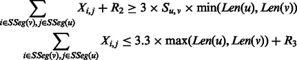 |
The two constraints are explained in Figure 3 as follows. Figure 3A shows that the total number of contacts between two β-strands diverges into two groups when  . One group is due to β-strand pairs forming a β-sheet. The other may be due to incorrectly predicted β-strands or β-strand pairs not in a β-sheet. Figure 3B shows that the total number of contacts between a pair of β-strands has an upper bound proportional to the length of the longer β-strand. As there are points below the skew line in Figure 3A, which indicate that a β-strand pair may have fewer than
  contacts, we add a relaxation variable
  to the lower bound constraints in Group 2. Similarly, we use a relaxation variable
  for the upper bound constraints.
Fig. 3.

The skew lines indicate the bounds for the total number of contacts between two β-strands. (A) Lower bound; (B) upper bound
Group 3. When two strands form an anti-parallel β-sheet, the contacts of neighboring residue pairs shall satisfy the following constraints.
where  are residues in one strand, and
  are residues in the other strand.
Group 4. When there are parallel contacts between two strands, the contacts of neighboring residue pairs should satisfy the following constraints.
where  are residues in one strand, and
  are residues in the other strand.
Group 5. One β-strand  can form β-sheets with up to two other β-strands.
Group 6. There is no contact between the start and end residues of a loop segment u.
In our training set, there are totally ∼8000 loop segments, and only 3.4% of them have a contact between the start and end residues. To allow the rare cases, we use a relaxation variable  in the constraints.
Group 7. One residue  cannot have contacts with both j and j + 2 when j and j + 2 are in the same α helix.
Group 8. This group of constraints models the relationship among different groups of variables.
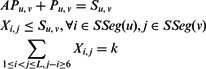 |
where k is the number of top contacts we want to predict.
Our ILP model is solved by IBM CPLEX academic version V12.1 (CPLEX, 2009).
Training data. It consists of 900 non-redundant protein structures, any two of which share no >25% sequence identity. As there are far fewer contacting residue pairs than non-contacting pairs, we use all the contacting pairs and randomly sample only 20% of the non-contacting pairs as the training data. All the training proteins are selected before CASP10 (the 10th Critical Assessment of Structure Prediction) started in May 2012.
Test data I: CASP10. This set contains 123 CASP10 targets with publicly available native structures. Meanwhile, 36 of them are classified as hard targets because the top half of their submitted models have average TM-score <0.5. When they were just released, most of the CASP10 targets share low sequence identity (<25%) with the proteins in PDB. BLAST indicates that there are only five short CASP10 targets (∼50 residues), which have sequence identity slightly >30% with our training proteins.
Test data II: Set600. This set contains 601 proteins randomly extracted from PDB25 (Brenner et al., 2000) and was constructed before CASP10 started. The test proteins have the following properties: (i) they share <25% sequence identity with the training proteins; (iii) all proteins have at least 50 residues and an X-ray structure with resolution better than 1.9 Å; and (iii) all the proteins have at least five residues with predicted secondary structure being α-helix or β-strand.
Both the training set and Set600 are sampled from PDB25 (Wang and Dunbrack, 2003), in which any two proteins share <25% sequence identity. Sequence identity is calculated using the method in (Brenner et al., 2000).
Programs to be compared. We compare our method, denoted as PhyCMAP, with four state-of-the-art methods: CMAPpro (Di Lena et al., 2012), NNcon (Tegge et al., 2009), PSICOV (Jones et al., 2012) and Evfold (Morcos et al., 2011). We run NNcon, PSICOV and Evfold locally and CMAPpro through its web server. We do not compare our method with Astro-Fold because it is not publicly available. Further, it does not perform well because of lack of evolutionary information.
Evaluation methods. Depending on the chain distance of the two residues, there are three kinds of contacts: short-range, medium-range and long-range. Short-range contacts are closely related to local conformation and are relatively easy to predict. Medium-range and long-range contacts determine the overall shape of a protein and are more challenging to predict. We evaluate prediction accuracy using the top 5, L/10, L/5 predicted contacts, where L is the protein length.
Meff: the number of non-redundant sequence homologs. Given a target and the multiple sequence alignment of all of its homologs, we measure the number of non-redundant sequence homologs by Meff as follows.
| (1) |
where both i and j go over all the sequence homologs, and Si,j is a binary similarity value between two proteins. Following Evfold (Morcos et al., 2011), we compute the similarity of two sequence homologs using their hamming distance. That is, Si,j is 1 if the normalized hamming distance is <0.3; 0 otherwise.
3 RESULTS
Performance on the CASP10 set. As shown in Table 3, on the whole-CASP10 set, our PhyCMAP significantly exceeds the second best method CMAPpro in terms of the accuracy of the top five, L/10 and L/5 predicted contacts. The advantage of PhyCMAP over CMAPpro becomes smaller but still substantial when short-range contacts are excluded from consideration. PhyCMAP significantly outperforms NNcon, PSICOV and Evfold no matter how the performance is evaluated.
Table 3.
This table lists the prediction accuracy of PhyCMAP, PSICOV, NNcon, CMAPpro and Evfold on short-, medium- and long-range contacts, tested on CASP10 (123 targets)
| Method | Short-range, sequence distance from 6 to 12 |
Medium- and long-range, sequence distance >12 |
Medium-range, sequence distance >12 and ≤24 |
Long-range, sequence distance >24 |
||||||||
|---|---|---|---|---|---|---|---|---|---|---|---|---|
| Top 5 | L/10 | L/5 | Top 5 | L/10 | L/5 | Top 5 | L/10 | L/5 | Top 5 | L/10 | L/5 | |
| PhyCMAP (Cα) | 0.623 | 0.555 | 0.459 | 0.650 | 0.584 | 0.523 | 0.585 | 0.518 | 0.448 | 0.421 | 0.363 | 0.320 |
| PhyCMAP (Cβ) | 0.667 | 0.580 | 0.482 | 0.655 | 0.604 | 0.539 | 0.621 | 0.550 | 0.465 | 0.514 | 0.425 | 0.373 |
| PSICOV (Cα) | 0.294 | 0.225 | 0.179 | 0.397 | 0.345 | 0.306 | 0.384 | 0.303 | 0.255 | 0.350 | 0.277 | 0.226 |
| PSICOV (Cβ) | 0.379 | 0.281 | 0.223 | 0.522 | 0.458 | 0.405 | 0.515 | 0.387 | 0.316 | 0.457 | 0.372 | 0.315 |
| NNcon (Cα) | 0.595 | 0.499 | 0.399 | 0.472 | 0.409 | 0.358 | 0.463 | 0.393 | 0.334 | 0.286 | 0.239 | 0.188 |
| CMAPpro (Cα) | 0.506 | 0.437 | 0.368 | 0.517 | 0.466 | 0.424 | 0.485 | 0.414 | 0.363 | 0.380 | 0.336 | 0.297 |
| CMAPpro (Cβ) | 0.543 | 0.477 | 0.395 | 0.519 | 0.466 | 0.415 | 0.491 | 0.419 | 0.370 | 0.395 | 0.347 | 0.313 |
| Evfold (Cα) | 0.236 | 0.193 | 0.165 | 0.380 | 0.326 | 0.295 | 0.351 | 0.294 | 0.249 | 0.328 | 0.257 | 0.225 |
Performance on the 36 hard CΑSP10 targets. As shown in Table 4, on the 36 hard CASP10 targets, our PhyCMAP exceeds the second best method CMAPpro by 5–7% in terms of the accuracy of the top five, L/10 and L/5 predicted contacts. The advantage of PhyCMAP over CMAPpro becomes smaller but still substantial when short-range contacts are excluded from consideration. PhyCMAP significantly outperforms NNcon, PSICOV and Evfold no matter how many predicted contacts are evaluated. PSICOV and Evfold almost fail on these hard CASP10 targets. By contrast, CMAPpro, NNcon and PhyCMAP still work, although they do not perform as well as on the whole CASP10 set.
Table 4.
Prediction accuracy on the 36 hard CASP10 targets
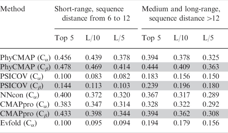 |
Note: The Cβ results are in gray rows.
Note that both PSICOV and Evfold, two recent methods receiving a lot of attentions from the community, do not perform well on the CASP10 set. This is partially because they require a large number of sequence homologs for the protein under prediction. Nevertheless, most of the CASP targets, especially the hard ones, do not have so many sequence homologs because a protein with so many homologs likely has similar templates in PDB and thus, were not used by CASP.
Relationship between prediction accuracy and the number of sequence homologs. We divide the 123 CASP10 targets into five groups according to their logMeff values: (0,2), (2,4), (4,6), (6,8), (8,10), which contain 19, 17, 25, 36 and 26 targets, respectively. Meanwhile, Meff is the number of non-redundant sequence homologs for the protein under consideration (see Section 2 for definition). Only medium- and long-range contacts are considered here. Figure 4 clearly shows that the prediction accuracy increases with respect to Meff. The more non-redundant homologs are available, the better prediction accuracy can be achieved by PhyCMAP, Evfold and PSICOV. However, CMAPpro and NNcon have decreased accuracy when logMeff >8.
Fig. 4.

The relationship between prediction accuracy and the number of non-redundant sequence homologs (Meff). x-axis is logMeff and y-axis is the mean accuracy of top L/10 predicted contacts on the corresponding CASP10 target group. Only medium- and long-range contacts are considered
Figure 4 also shows that PhyCMAP outperforms Evfold, CMAPpro and NNcon across all Meff. PhyCMAP greatly outperforms PSICOV in predicting Cα contacts regardless of Meff and also in predicting Cβ contacts when logMeff ≤6. PhyCMAP has comparable performance as PSICOV in predicting Cβ contacts when logMeff >6.
Performance on Set600. To fairly compare our method with Evfold (Morcos et al., 2011) and PSICOV (Jones et al., 2012), both of which require a large number of sequence homologs, we divide Set600 into two subsets based on the amount of homologous information available for the protein under prediction. The first subset is relatively easier, containing 471 proteins with Meff > 100 (see Section 2 for definition). All the proteins in this subset have >500 sequence homologs, which satisfies the requirement of PSICOV. The second subset is more challenging to predict, containing 130 proteins with Meff ≤ 100. As shown in Table 5, even on the first subset, PhyCMAP still exceeds PSICOV and Evfold, although the advantage over PSICOV is not substantial for Cβ contacts prediction when short-range contacts are excluded from consideration. PhyCMAP also outperforms NNcon and CMAPpro on this set. As shown in Table 6, on the second subset, PhyCMAP significantly outperforms PSICOV and is slightly better than CMAPpro and NNcon. These results again confirm that our method applies to a protein without many sequence homologs, on which PSICOV and Evfold usually fail.
Table 5.
Benchmark on the 471 proteins with Meff > 100
| Method | Short-range, sequence distance from 6 to 12 |
Medium- and long-range, sequence distance >12 |
||||
|---|---|---|---|---|---|---|
| Top 5 | L/10 | L/5 | Top 5 | L/10 | L/5 | |
| PhyCMAP (Cα) | 0.761 | 0.653 | 0.539 | 0.716 | 0.675 | 0.611 |
| PhyCMAP (Cβ) | 0.746 | 0.637 | 0.531 | 0.731 | 0.656 | 0.608 |
| PSICOV (Cα) | 0.457 | 0.341 | 0.257 | 0.528 | 0.465 | 0.411 |
| PSICOV (Cβ) | 0.584 | 0.425 | 0.316 | 0.732 | 0.646 | 0.565 |
| NNcon (Cα) | 0.512 | 0.432 | 0.355 | 0.432 | 0.361 | 0.308 |
| CMAPpro (Cα) | 0.682 | 0.551 | 0.431 | 0.710 | 0.642 | 0.574 |
| CMAPpro (Cβ) | 0.671 | 0.542 | 0.436 | 0.674 | 0.601 | 0.532 |
| Evfold (Cα) | 0.379 | 0.297 | 0.234 | 0.473 | 0.438 | 0.400 |
Table 6.
Benchmark on the 130 proteins with Meff ≤ 100
| Method | Short-range, sequence distance from 6 to 12 |
Medium- and long-range, sequence distance >12 |
||||
|---|---|---|---|---|---|---|
| Top 5 | L/10 | L/5 | Top 5 | L/10 | L/5 | |
| PhyCMAP (Cα) | 0.534 | 0.451 | 0.377 | 0.432 | 0.372 | 0.319 |
| PhyCMAP (Cβ) | 0.505 | 0.435 | 0.365 | 0.418 | 0.364 | 0.314 |
| PSICOV (Cα) | 0.060 | 0.061 | 0.064 | 0.049 | 0.039 | 0.035 |
| PSICOV (Cβ) | 0.077 | 0.070 | 0.073 | 0.069 | 0.050 | 0.045 |
| NNcon (Cα) | 0.442 | 0.363 | 0.309 | 0.368 | 0.339 | 0.301 |
| CMAPpro (Cα) | 0.435 | 0.365 | 0.314 | 0.368 | 0.331 | 0.300 |
| CMAPpro (Cβ) | 0.532 | 0.434 | 0.353 | 0.358 | 0.331 | 0.280 |
Note: The result for Evfold is not shown, as it does not produce meaningful predictions for some proteins.
It should be noticed that CMAPpro used Astral 1.73 (Brenner et al., 2000; Di Lena et al., 2012) as its training set, which shares >90% sequence identity with 226 proteins in Set600 (180 with Meff > 100 and 46 with Meff ≤ 100). To more fairly compare the prediction methods, we exclude the 226 proteins from Set600 that share >90% sequence identity with the CMAPpro training set. Here, the sequence identity is calculated using CD-HIT (Li and Godzik, 2006; Li et al., 2001). This results in a set of 291 proteins with Meff > 100 and 84 proteins Meff ≤ 100. Table 7 shows that PhyCMAP greatly outperforms CMAPpro and Evfold on the reduced dataset. PhyCMAP also outperforms PSICOV in predicting Cα contacts, but it is slightly worse in predicting long-range Cβ contacts.
Table 7.
This table lists the prediction accuracy of PhyCMAP, PSICOV, NNcon, CMAPpro and Evfold on short-, medium- and long-range contacts, tested on Set600
| Method | Short-range, sequence distance from 6 to 12 |
Medium- and long-range, sequence distance >12 |
Medium-range, sequence distance >12 and ≤24 |
Long-range, sequence distance >24 |
||||||||
|---|---|---|---|---|---|---|---|---|---|---|---|---|
| Top 5 | L/10 | L/5 | Top 5 | L/10 | L/5 | Top 5 | L/10 | L/5 | Top 5 | L/10 | L/5 | |
| a) The 291 proteins in Set600 with Meff >100 and ≤90% sequence identify with Astral 1.73 | ||||||||||||
| PhyCMAP(Cα) | 0.759 | 0.653 | 0.536 | 0.713 | 0.680 | 0.622 | 0.639 | 0.570 | 0.496 | 0.582 | 0.528 | 0.461 |
| PhyCMAP(Cβ) | 0.741 | 0.641 | 0.534 | 0.746 | 0.653 | 0.611 | 0.655 | 0.571 | 0.500 | 0.636 | 0.550 | 0.477 |
| PSICOV(Cα) | 0.459 | 0.343 | 0.258 | 0.528 | 0.469 | 0.417 | 0.462 | 0.363 | 0.282 | 0.483 | 0.418 | 0.358 |
| PSICOV(Cβ) | 0.582 | 0.422 | 0.314 | 0.733 | 0.650 | 0.569 | 0.647 | 0.496 | 0.371 | 0.674 | 0.584 | 0.495 |
| NNcon(Cα) | 0.475 | 0.390 | 0.318 | 0.377 | 0.313 | 0.267 | 0.342 | 0.284 | 0.236 | 0.224 | 0.182 | 0.152 |
| CMAPpro(Cα) | 0.643 | 0.519 | 0.412 | 0.689 | 0.618 | 0.554 | 0.580 | 0.511 | 0.439 | 0.527 | 0.469 | 0.416 |
| CMAPpro(Cβ) | 0.642 | 0.520 | 0.422 | 0.653 | 0.580 | 0.515 | 0.573 | 0.494 | 0.421 | 0.504 | 0.444 | 0.396 |
| Evfold(Cα) | 0.382 | 0.297 | 0.235 | 0.488 | 0.442 | 0.398 | 0.451 | 0.366 | 0.289 | 0.442 | 0.389 | 0.342 |
| b) The 84 proteins in Set600 with Meff ≤100 and ≤90% sequence identity with Astral 1.73 | ||||||||||||
| PhyCMAP(Cα) | 0.580 | 0.488 | 0.404 | 0.481 | 0.430 | 0.357 | 0.476 | 0.417 | 0.335 | 0.204 | 0.179 | 0.159 |
| PhyCMAP(Cβ) | 0.548 | 0.468 | 0.392 | 0.454 | 0.408 | 0.345 | 0.452 | 0.399 | 0.331 | 0.220 | 0.214 | 0.187 |
| PSICOV(Cα) | 0.070 | 0.071 | 0.072 | 0.065 | 0.050 | 0.044 | 0.074 | 0.055 | 0.049 | 0.063 | 0.043 | 0.035 |
| PSICOV(Cβ) | 0.081 | 0.078 | 0.083 | 0.088 | 0.068 | 0.059 | 0.092 | 0.066 | 0.059 | 0.076 | 0.058 | 0.046 |
| NNcon(Cα) | 0.535 | 0.421 | 0.342 | 0.324 | 0.298 | 0.248 | 0.348 | 0.321 | 0.271 | 0.162 | 0.132 | 0.114 |
| CMAPpro(Cα) | 0.465 | 0.370 | 0.316 | 0.346 | 0.328 | 0.285 | 0.360 | 0.332 | 0.286 | 0.173 | 0.169 | 0.158 |
| CMAPpro(Cβ) | 0.447 | 0.367 | 0.321 | 0.346 | 0.320 | 0.287 | 0.366 | 0.331 | 0.290 | 0.191 | 0.189 | 0.176 |
| Evfold(Cα) | 0.074 | 0.068 | 0.066 | 0.079 | 0.058 | 0.039 | 0.074 | 0.053 | 0.045 | 0.063 | 0.042 | 0.032 |
3.1 Contribution of contrastive mutual information and pairwise contact scores
The CMI and HPS help improve the performance of our RF model. Table 8 shows their contribution to the prediction accuracy on the 471 proteins (with Meff > 100) in Set600.
Table 8.
The contribution of CMI and homologous pair contact scores to Cβ contact prediction
| Method | Short-range contacts |
Medium- and long-range |
||||
|---|---|---|---|---|---|---|
| Top 5 | L/10 | L/5 | Top 5 | L/10 | L/5 | |
| with CMI and HPS | 0.754 | 0.632 | 0.521 | 0.720 | 0.649 | 0.589 |
| no CMI and HPS | 0.600 | 0.570 | 0.487 | 0.538 | 0.560 | 0.506 |
Note: Similar results are observed for Cα contact prediction.
3.2 Contribution of physical constraints
Table 9 shows the improvement resulting from the physical constraints (i.e. the ILP method) over the RF method on Set600. On the 471 proteins with Meff > 100, ILP improves medium and long-range contact prediction, but not short-range contact prediction. This result confirms that the physical constraints used by our ILP method indeed capture some global properties of a protein contact map. The improvement resulting from the physical constraints is larger on the 130 proteins with Meff ≤ 100. In particular, the improvement on short-range contacts is substantial. These results may imply that when homologous information is sufficient, we can predict short-range contacts accurately and thus, cannot further improve the prediction by using the physical constraints. When homologous information is insufficient for accurate contact prediction, we can improve the prediction using the physical constraints, which are complementary to evolutionary information.
Table 9.
The contribution of physical constraints
| Method | Short-range contacts |
Medium- and long-range |
||||
|---|---|---|---|---|---|---|
| Top 5 | L/10 | L/5 | Top 5 | L/10 | L/5 | |
471 proteins in Set600 with Meff
 100 100 | ||||||
| RF + ILP | 0.746 | 0.637 | 0.531 | 0.731 | 0.656 | 0.608 |
| RF | 0.754 | 0.632 | 0.521 | 0.720 | 0.649 | 0.589 |
| 130 proteins in Set600 with Meff ≤ 100 | ||||||
| RF + ILP | 0.505 | 0.435 | 0.365 | 0.418 | 0.364 | 0.314 |
| RF | 0.445 | 0.368 | 0.299 | 0.414 | 0.342 | 0.281 |
Note: The results are Cβ contact prediction.
3.3 Specific examples
We show the contact prediction results of two CASP10 targets T0693D2 and T0677D2 in Figures 5 and 6, respectively. T0693D2 has many sequence homologs with Meff = 2208.39. As shown in Figure 5, PhyCMAP does well in predicting the long-distance contacts around the residue pair (20,100). For this target, PhyCMAP and Evfold obtain top L/10 prediction accuracy of 0.810 and 0.619, respectively, on medium- and long-range contacts. T0677D2 does not have many sequence homologs with Meff = 31.53. As shown in Figure 6, our prediction matches well with the native contacts. PhyCMAP has top L/10 prediction accuracy 0.429 on medium- and long-range contacts, whereas Evfold cannot correctly predict any contacts.
Fig. 5.

The predicted medium- and long-range contacts for T0693D2. The upper triangles display the native Cβ contacts. The lower triangles of the left and right plots display the contact probabilities predicted by PhyCMAP and Evfold, respectively
Fig. 6.

The predicted medium- and long-range contacts for T0677D2. The upper triangles display the native Cβ contacts. The lower triangles of the left and right plots display the contact probabilities predicted by PhyCMAP and Evfold, respectively
4 CONCLUSION AND DISCUSSIONS
This article has presented a novel method for protein contact map prediction by integrating both evolutionary and physical constraints using machine learning and ILP. Our method differs from currently popular contact prediction methods in that we enforce a few physical constraints, which imply the sparsity constraint (used by PSICOV and Evfold), to the whole-contact map and take into consideration contact correlation. Our method also differs from the first-principle method (e.g. Astro-Fold) in that we exploit evolutionary information from several aspects (e.g. MI, context-specific distance potential and sequence profile) to significantly improve prediction accuracy. Experimental results confirm that our method outperforms existing popular machine-learning methods (e.g. CMAPpro and NNcon) and two recent co-mutation–based methods PSICOV and Evfold regardless of the number of sequence homologs available for the protein under consideration.
The study of our method indicates that the physical constraints are helpful for contact prediction, especially when the protein under consideration does not have many sequence homologs. Nevertheless, the physical constraints exploited by our current method do not cover all the properties of a protein contact map. To further improve prediction accuracy on medium- and long-range contact prediction, we may take into consideration global properties of a protein distance matrix. For example, the pairwise distances of any three residues shall satisfy the triangle inequality. Some residues also have correlated pairwise distances. To enforce this kind of distance constraints, we shall introduce distance variables and also define their relationship with contact variables. By introducing distance variables, we may also optimize the distance probability, as opposed to the contact probability used by our current ILP method. Further, we can also introduce variables of β-sheet (group of β-strands) to capture more global properties of a contact map.
One may ask how our approach compares with a model-based filtering strategy in which 3D models are built based on initial predicted contacts and then used to filter incorrect predictions. Our method differs from this general ‘model-based filtering’ strategy in a couple of aspects. First, it is time-consuming to build thousands or at least hundreds of 3D models with initial predicted contacts. In contrast, our method can do contact prediction (using physical constraints) within minutes. Second, the quality of the 3D models is also determined by other factors, such as energy function and energy optimization (or conformation sampling) methods, whereas our method is independent of these factors. Even if the energy function is accurate, the energy optimization algorithm often is trapped to local minima because the energy function is not rugged. That is, the 3D models resulting from energy minimization are biased toward a specific region of the conformation space, unless an extremely large-scale of conformation sampling is conducted. Therefore, the predicted contacts derived from these models may also suffer from this ‘local minima’ issue. By contrast, our integer programming method can search through the whole conformation space and find the global optimal solution; thus, it is not biased to any local minima region. By using our predicted contacts as constraints, we may pinpoint to the good region of a conformation space (without being biased by local minima), reduce the search space and significantly speed-up conformation search.
ACKNOWLEDGEMENTS
The authors are grateful to anonymous reviewers for their insightful comments and to the University of Chicago Beagle team and TeraGrid for their support of computational resources.
Funding: National Institutes of Health (R01GM0897532); National Science Foundation DBI-0960390; NSF CAREER award CCF-1149811; Alfred P. Sloan Research Fellowship.
Conflict of Interest: none declared.
REFERENCES
- Altschul SF, Koonin EV. Iterated profile searches with PSI-BLAST—a tool for discovery in protein databases. Trends Biochem. Sci. 1998;23:444–447. doi: 10.1016/s0968-0004(98)01298-5. [DOI] [PubMed] [Google Scholar]
- Baú D, et al. Distill: a suite of web servers for the prediction of one-, two-and three-dimensional structural features of proteins. BMC Bioinformatics. 2006;7:402. doi: 10.1186/1471-2105-7-402. [DOI] [PMC free article] [PubMed] [Google Scholar]
- Breiman L. Random forests. Mach. Learn. 2001;45:5–32. [Google Scholar]
- Brenner SE, et al. The ASTRAL compendium for protein structure and sequence analysis. Nucleic Acids Res. 2000;28:254–256. doi: 10.1093/nar/28.1.254. [DOI] [PMC free article] [PubMed] [Google Scholar]
- Caprara A, et al. 1001 optimal PDB structure alignments: integer programming methods for finding the maximum contact map overlap. J. Comput. Biol. 2004;11:27–52. doi: 10.1089/106652704773416876. [DOI] [PubMed] [Google Scholar]
- Cheng J, Baldi P. Improved residue contact prediction using support vector machines and a large feature set. BMC Bioinformatics. 2007;8:113. doi: 10.1186/1471-2105-8-113. [DOI] [PMC free article] [PubMed] [Google Scholar]
- International Business Machines Corporation. V12. 1: User’s Manual for CPLEX. 2009. IBM ILOG CPLEX. [Google Scholar]
- Di Lena P, et al. Deep architectures for protein contact map prediction. Bioinformatics. 2012;28:2449–2457. doi: 10.1093/bioinformatics/bts475. [DOI] [PMC free article] [PubMed] [Google Scholar]
- Fariselli P, Casadio R. A neural network based predictor of residue contacts in proteins. Protein Eng. 1999;12:15–21. doi: 10.1093/protein/12.1.15. [DOI] [PubMed] [Google Scholar]
- Göbel U, et al. Correlated mutations and residue contacts in proteins. Proteins. 2004;18:309–317. doi: 10.1002/prot.340180402. [DOI] [PubMed] [Google Scholar]
- Jones DT. Protein secondary structure prediction based on position-specific scoring matrices. J. Mol. Biol. 1999;292:195–202. doi: 10.1006/jmbi.1999.3091. [DOI] [PubMed] [Google Scholar]
- Jones DT, et al. PSICOV: precise structural contact prediction using sparse inverse covariance estimation on large multiple sequence alignments. Bioinformatics. 2012;28:184–190. doi: 10.1093/bioinformatics/btr638. [DOI] [PubMed] [Google Scholar]
- Klepeis J, Floudas C. ASTRO-FOLD: a combinatorial and global optimization framework for ab initio prediction of three-dimensional structures of proteins from the amino acid sequence. Biophys. J. 2003;85:2119–2146. doi: 10.1016/s0006-3495(03)74640-2. [DOI] [PMC free article] [PubMed] [Google Scholar]
- Li W, Godzik A. Cd-hit: a fast program for clustering and comparing large sets of protein or nucleotide sequences. Bioinformatics. 2006;22:1658–1659. doi: 10.1093/bioinformatics/btl158. [DOI] [PubMed] [Google Scholar]
- Li W, et al. Clustering of highly homologous sequences to reduce the size of large protein databases. Bioinformatics. 2001;17:282–283. doi: 10.1093/bioinformatics/17.3.282. [DOI] [PubMed] [Google Scholar]
- Liaw A, Wiener M. Classification and regression by randomforest. R News. 2002;2:18–22. [Google Scholar]
- Morcos F, et al. Direct-coupling analysis of residue coevolution captures native contacts across many protein families. Proc. Natl. Acad. Sci. USA. 2011;108:E1293–E1301. doi: 10.1073/pnas.1111471108. [DOI] [PMC free article] [PubMed] [Google Scholar]
- Olmea O, Valencia A. Improving contact predictions by the combination of correlated mutations and other sources of sequence information. Fold. Des. 1997;2:S25–S32. doi: 10.1016/s1359-0278(97)00060-6. [DOI] [PubMed] [Google Scholar]
- Ortiz AR, et al. Ab initio folding of proteins using restraints derived from evolutionary information. Proteins. 1999;37:177–185. doi: 10.1002/(sici)1097-0134(1999)37:3+<177::aid-prot22>3.3.co;2-5. [DOI] [PubMed] [Google Scholar]
- Punta M, Rost B. PROFcon: novel prediction of long-range contacts. Bioinformatics. 2005;21:2960–2968. doi: 10.1093/bioinformatics/bti454. [DOI] [PubMed] [Google Scholar]
- Tan YH, et al. Statistical potential-based amino acid similarity matrices for aligning distantly related protein sequences. Proteins. 2006;64:587–600. doi: 10.1002/prot.21020. [DOI] [PubMed] [Google Scholar]
- Tegge AN, et al. NNcon: improved protein contact map prediction using 2D-recursive neural networks. Nucleic Acids Res. 2009;37:W515–W518. doi: 10.1093/nar/gkp305. [DOI] [PMC free article] [PubMed] [Google Scholar]
- Vassura M, et al. Reconstruction of 3D structures from protein contact maps. IEEE/ACM Trans. Comput. Biol. Bioinform. 2008;5:357–367. doi: 10.1109/TCBB.2008.27. [DOI] [PubMed] [Google Scholar]
- Vendruscolo M, Domany E. Pairwise contact potentials are unsuitable for protein folding. J. Chem. Phys. 1998;109:11101. [Google Scholar]
- Vendruscolo M, et al. Recovery of protein structure from contact maps. Fold. Des. 1997;2:295–306. doi: 10.1016/S1359-0278(97)00041-2. [DOI] [PubMed] [Google Scholar]
- Vullo A, et al. A two-stage approach for improved prediction of residue contact maps. BMC Bioinformatics. 2006;7:180. doi: 10.1186/1471-2105-7-180. [DOI] [PMC free article] [PubMed] [Google Scholar]
- Wang G, Dunbrack RL., Jr. PISCES: a protein sequence culling server. Bioinformatics. 2003;19:1589–1591. doi: 10.1093/bioinformatics/btg224. [DOI] [PubMed] [Google Scholar]
- Wang S, et al. Protein structure alignment beyond spatial proximity. Sci. Rep. 2013;3:1448. doi: 10.1038/srep01448. [DOI] [PMC free article] [PubMed] [Google Scholar]
- Wu S, et al. Improving protein structure prediction using multiple sequence-based contact predictions. Structure. 2011;19:1182–1191. doi: 10.1016/j.str.2011.05.004. [DOI] [PMC free article] [PubMed] [Google Scholar]
- Wu S, Zhang Y. A comprehensive assessment of sequence-based and template-based methods for protein contact prediction. Bioinformatics. 2008;24:924–931. doi: 10.1093/bioinformatics/btn069. [DOI] [PMC free article] [PubMed] [Google Scholar]
- Xu J, et al. A parameterized algorithm for protein structure alignment. J. Comput. Biol. 2007;14:564–577. doi: 10.1089/cmb.2007.R003. [DOI] [PubMed] [Google Scholar]
- Zhao F, Xu J. A position-specific distance-dependent statistical potential for protein structure and functional study. Structure. 2012;20:1118–1126. doi: 10.1016/j.str.2012.04.003. [DOI] [PMC free article] [PubMed] [Google Scholar]
- Zhou H, Skolnick J. Protein model quality assessment prediction by combining fragment comparisons and a consensus Cα contact potential. Proteins. 2007;71:1211–1218. doi: 10.1002/prot.21813. [DOI] [PMC free article] [PubMed] [Google Scholar]