Using state machines to model the Ion Torrent sequencing process and to improve read error rates

Abstract

Motivation: The importance of fast and affordable DNA sequencing methods for current day life sciences, medicine and biotechnology is hard to overstate. A major player is Ion Torrent, a pyrosequencing-like technology which produces flowgrams – sequences of incorporation values – which are converted into nucleotide sequences by a base-calling algorithm. Because of its exploitation of ubiquitous semiconductor technology and innovation in chemistry, Ion Torrent has been gaining popularity since its debut in 2011. Despite the advantages, however, Ion Torrent read accuracy remains a significant concern.

Results: We present FlowgramFixer, a new algorithm for converting flowgrams into reads. Our key observation is that the incorporation signals of neighboring flows, even after normalization and phase correction, carry considerable mutual information and are important in making the correct base-call. We therefore propose that base-calling of flowgrams should be done on a read-wide level, rather than one flow at a time. We show that this can be done in linear-time by combining a state machine with a Viterbi algorithm to find the nucleotide sequence that maximizes the likelihood of the observed flowgram. FlowgramFixer is applicable to any flowgram-based sequencing platform. We demonstrate FlowgramFixer’s superior performance on Ion Torrent Escherichia coli data, with a 4.8% improvement in the number of high-quality mapped reads and a 7.1% improvement in the number of uniquely mappable reads.

Availability: Binaries and source code of FlowgramFixer are freely available at: http://www.cs.tau.ac.il/~davidgo5/flowgramfixer.html.

Contact: davidgo5@post.tau.ac.il

1 INTRODUCTION

The importance of fast and affordable DNA sequencing methods for current day life sciences, medicine and biotechnology is hard to overstate. Ion Torrent’s semiconductor sequencing technology, as implemented in its Personal Genome Machine (PGM), has been gaining popularity as a fast and affordable sequencing platform since it’s debut in 2011 (Merriman et al., 2012; Rothberg et al., 2011). Semiconductor sequencing has several advantages compared with other high-throughput sequencing platforms, including lack of optics, use of natural, unmodified dNTP molecules and exploitation of ubiquitous semiconductor technology. These advances make Ion Torrent a serious player in the sequencer market, providing reads several hundred bases long and reducing sequencing costs (Eisenstein, 2012).

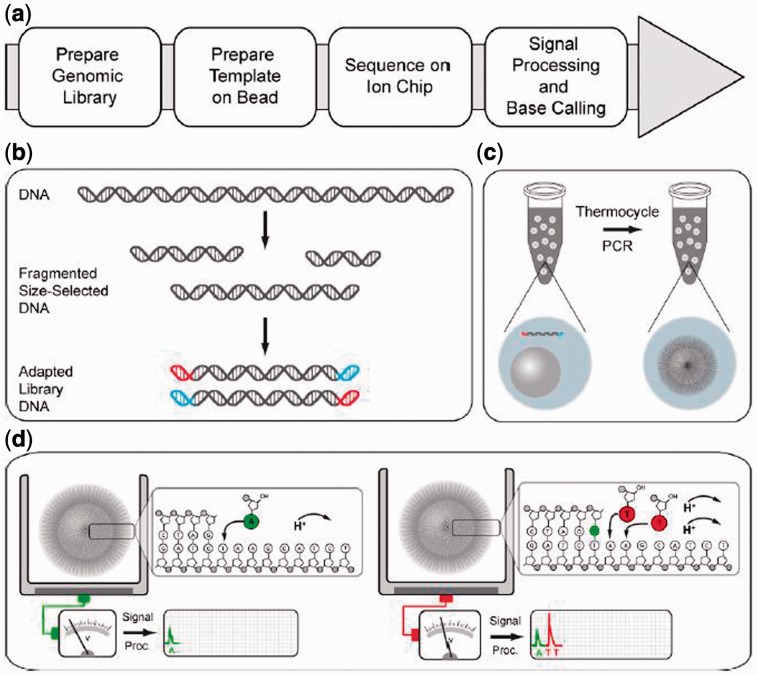
Ion Torrent is a pyrosequencing-like platform, similar to 454. In every sequencing step, or flow, the chip is washed over with a specific nucleotide. The nucleotide in the flow is incorporated by all consecutive complementary nucleotides ‘hanging’ at the end of each template—this is called incorporation. Each incorporation releases an ion, so that the change in pH level indicates whether incorporation occurred and, if so, the number of consecutive bases incorporated. The nucleotide that is washed during each flow is pre-determined and is composed from several repetitions of a shorter sequence of nucleotides known as the ‘wash cycle’. The default wash cycle for 454 is 4 nt long: , whereas Ion Torrent’s PGM uses a more complicated wash cycle that is 32 nt long. The resulting read is then specified in terms of a flowgram—a sequence of incorporation values, one for each flow. Figure 1 gives an overview of the process.

Fig. 1.

Ion sequencing work flow. The overall workflow is shown in (a). A genome library is prepared by fragmenting and size-selecting DNA, followed by the ligation of forward and reverse adapters (b). Each adapter-ligated template is clonally amplified onto a bead, so that each bead contains many copies of the same DNA template (c). Sequence on the chip, sequencing primers and DNA polymerase are then bound to the beads, which are pipetted into wells on the chip (d). The chip is then repeatedly flooded by nucleotides, which, when binding to the complementary nucleotide on a template, release an ion. At each flow, the electrical signal at each well is measured, indicating the number of incorporations [Figure adapted from Rothberg et al. (2011)]

Despite its advantages, Ion Torrent read accuracy remains a significant concern. Errors are produced during base-calling, a process by which the noisy signal from the sequencer is converted into a sequence of nucleotides. Base-calling errors can especially pose challenges for re-sequencing projects, where they can be confused with SNPs. In fact, a recent comparative study found that Ion Torrent’s PGM still suffers from high–false-positive rates in SNP calling, relative to Illumina data (Quail et al., 2012). There is a large body of work on base-calling algorithms [see Ledergerber and Dessimoz (2011) for a survey], and there have been several techniques developed specifically for pyrosequencing data (Beuf et al., 2012; Lysholm et al., 2011; Quince et al., 2011; Quinlan et al., 2008; Vacic et al., 2008). These techniques have mostly focused on correcting 454’s well-documented (Balzer et al., 2010) errors in long homopolymer runs or alignment of their flowgrams. However, there has been little work done in correcting base-calling errors in Ion Torrent data.

Ion Torrent’s base-calling algorithm, after performing phase-correction and normalizing to handle signal decay, simply translates the rounded values of each flow into the corresponding number of consecutive nucleotides. In essence, it is a memoryless algorithm that makes a call for each flow independent of information from previous or following flows. Our key observation is that the signals of neighboring flows carry considerable mutual information and are important in making the correct base-call. We propose that base-calling of flowgrams should be done on a read-wide level, rather than one flow at a time. To this end, we design a linear-time method that combines a state machine with a Viterbi algorithm to find the nucleotide sequence that maximizes the likelihood of the observed flowgram. Our algorithm is applicable to any flowgram-based sequencing platform and is implemented in a publicly available tool called FlowgramFixer. We demonstrate FlowgramFixer’s superior performance on Ion Torrent Escherichia coli data, with a 4.8% improvement in the number of high-quality mapped reads and a 7.1% improvement in the number of uniquely mappable reads.

2 BACKGROUND AND MOTIVATING EXAMPLES

We denote the set of possible DNA sequences by ‘nt-space’, i.e. the space of possible combinations of the four nucleotides A, C, G and T. The Ion Torrent platform does not provide us directly with the read in nucleotide space, but instead, we observe the incorporation signal at each flow. It is, therefore, useful to define ‘flow-space’, as the vector of incorporation signals (flowgram) obtained per flow by a perfect (noiseless) sequencing process. For example, if the flow nucleotides are two repetitions of the wash cycle ‘ACGT’, and the sequence itself is GCCT, then the flow-space representation is (0,0,1,0,0,2,0,1).

The actual signal is noisy; therefore, the observed flowgram is not a sequence of integers, but rather a sequence of non-negative real values. The noise is due to a range of artifacts. First, Ion Torrent’s platform uses discrete time measurements from the pH sensors at the bottom of each well to fit a theoretical physical model of a continuous time process (nucleotide incorporation). The process of nucleotide incorporation is random by nature and is affected by various factors ranging from random changes of dNTP molecule concentration to random fluctuations in fluid-dynamics because of bubbles or turbulences. And so, the theoretical physical model does not capture the full complexity of the sequencing process and does not always fit the observed signals perfectly, resulting in noisy signal.

Second, the signal decays over time, as at each flow a small fraction of the template clones attached to each bead are terminated and no longer incorporate additional nucleotides (this phenomenon is known as ‘drooping’). Thus, the actual signal observed at each flow decays over time. Although this phenomenon is not by itself a source of noise, the decay of the signal decreases the signal-to-noise ratio, making correct calling harder as the sequencing process progresses.

Finally, some of the template clones drop out of phase as the sequencing progresses. Even when the current nucleotide in the flow should be incorporated by all template clones, clones might not, by chance, incorporate it (for example, if no dNTP molecule is found in the physical vicinity of the template). These clones would incorporate the nucleotide at the next flow of the same nucleotide. Hence, the signal becomes unphased—the observed signal is a superposition of lagged copies of the true signal, where the lags depend on the wash cycle and the underlying sequence itself.

As the initial step of its base-calling software, Ion Torrent performs phase-correction and signal decay normalization algorithms. A typical flowgram, after this correction, is shown in Figure 2. The resulting incorporation values are still noisy, and, to convert them to nucleotide space, Ion Torrent rounds them to the nearest integer. Although this last step is effective and scalable, we find that it is suboptimal for several reasons.

Fig. 2.

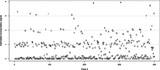
Typical flowgram. We show the normalized and phase-corrected signal of a single flowgram. The actual nucleotide in each flow is indicated by the appropriate letter. Ideal signals are expected to be integers, indicating exactly how many nucleotides were incorporated during each flow. However, the actual signal at each flow is noisy, and the noise increases as the sequencing process advances

First, rounding the signal flow-by-flow might result in an ‘impossible’ sequence of signals. Consider the following toy example, where the first nucleotide is T and the wash cycle is ACGT. The expected signal is (0,0,0,1)—no incorporation in the first three flows, and an incorporation of a single nucleotide in the fourth flow. Next, imagine that because of noise, the measured signal is (0.1,0.05,0.08,0.4). Rounding the signal would result in (0,0,0,0). Such a flow-sequence implies that the first nucleotide cannot be A, C, G or T—an impossibility. However, by observing the whole sequence of incorporation values together, we would have been able to deduce that the fourth incorporation of 0.4 should be rounded up, not down.

Second, the probability of observing an incorporation event depends on the incorporation signals of previous and next flows. Assume, for example, the same flow order as before, and assume that we have seen incorporations in the first three flows. This implies that the sequence starts with ACG, and that the next base in the sequence is not G (otherwise we would have seen two incorporation events in the third flow). Therefore, there are three possible candidates for the next nucleotide—A, C and T. Next, assume a different scenario—an incorporation event happened only in the second flow, with no incorporation in the first and third flows. In this case, the sequence starts with C, and the second nucleotide cannot be G (otherwise we would have seen an incorporation in the third flow), and it cannot be C (otherwise we would have seen two incorporations in the second flow). Hence, there are only two candidates for the next nucleotide—A and T. In the first scenario, the previous probability of observing an incorporation in the fourth flow is , as T is one of three possible nucleotides, whereas in the second scenario, the previous probability is , as T is one of only two possible nucleotides. Simply rounding the signal at each flow to the nearest integer ignores the previous probability obtained by considering the incorporations at previous flows. Future flows also carry useful information regarding a current flow in a similar manner.

Finally, rounding signals ignores other previous information regarding the genome, such as GC-content and the lower frequencies of longer homopolymers. One can think of the rounding method as setting a threshold of 0.5 and calling an incorporation event when the incorporation signal is higher than the threshold. When sequencing genomes that are known to be GC-rich, it is reasonable to use different thresholds for flows with different washed nucleotides. For example, when the flow is either G or C, an incorporation event is more likely before observing the signal, compared with flows of A or T. Similarly, longer homopolymers are less likely; therefore, the threshold for calling 0mer versus 1mer need not be the same threshold as the one used in calling 5mer versus 6mer [similar to what is done for 454 reads by Quinlan et al. (2008) and others].

3 METHODS

Motivated by the examples of the previous section, we develop a method that finds a nucleotide sequence that maximizes the likelihood of the observed flowgram. We start by describing the underlying state machine that captures the sequencing process. We then define the distributions necessary for calculating the likelihood. Finally, we describe two dynamic programming algorithms—a Viterbi algorithm to find the maximum likelihood nucleotide sequence, and a forward algorithm to obtain maximum-likelihood estimates of the noise-model parameters.

3.1 State machine model

To connect flow-space and nucleotide-space, one can ask, at each flow, what are the different possibilities for the next nucleotide. For instance, at the first flow, we have no information at all, and the first base of the sequence could be A, C, G or T. If the first flow presents no incorporation, the possible candidates become C, G and T and so forth. This process is illustrated on our previous toy example in Table 1.

Table 1.

Representing the set of possible nucleotides after each flow

Flow No.	Flow nucleotide	Candidates	Remaining sequence	Signal
1	A	ACGT	GCCT	0
2	C	CGT	GCCT	0
3	G	GT	GCCT	1
4	T	ACT	CCT	0
5	A	AC	CCT	0
6	C	C	T	2
7	G	AGT	T	0
8	T	AT	—	1

Note: Here, the wash cycle is ACGT and the sequenced string is GCCT. Initially, any nucleotide is possible—the candidates are ACGT. The first flow (A) produces no incorporation signal; therefore, the candidates for the next nucleotide are CGT. After an incorporation event, as in flows 3 and 6, the candidate nucleotides for the next base in the sequence are all the nucleotides except for the one that was just incorporated.

More generally, we define a deterministic state machine (Hopcroft and Ullman, 1979). There are 15 states, corresponding to the possible sets of candidate nucleotides. Each state represents the possible nucleotides for the next position, in nucleotide-space. It is convenient to think of the binary representation of the number as indicating which nucleotides are candidates, or, alternatively, as an actual set containing the appropriate subset of base letters. The initial state is . Given a flow nucleotide, a state s can transition to at most two states, one where an incorporation occurs, denoted , and one where no incorporation occurs, denoted . For example, when the state is , and the flow nucleotide is A, the next state can be either (if there is an incorporation event, A is now the only non-candidate) or (if there is no incorporation event, A is no longer a candidate). When the flow nucleotide is not one of the candidates given by the current state, there is no incorporation transition. Thus, each state has at most eight outgoing transitions.

A path in the state machine is a sequence of transitions from the initial state. Given a wash cycle, a flow-sequence defines a path in the state machine in the obvious manner. Figure 3 illustrates the transitions of a state machine on a simple wash cycle.

Fig. 3.

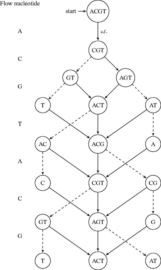
Illustration of state machine transitions. In this example, the flow is composed of repetitions of the wash cycle ACGT and the state machine starts from the state {A,C,G,T}. Each layer of the figure illustrates the possible states at that flow index. Incorporation and no incorporation transitions are marked by solid and dashed edges, respectively. Note that nodes with a single nucleotide dictate incorporation in the next flow and have no outgoing dashed edges

3.2 Problem formulation

Let denote the observed (normalized and phase-corrected) incorporation values, with being the true (noiseless) values in flow-space. F defines a path in the state machine, , where s_i is the state after the application of flow f_i. We let s₀ be the initial state before any incorporations, i.e. . The likelihood of the flows F given the observed values O is given by:

where is the probability of transition from state to state s_i, π is a previous distribution over the lengths of homopolymers in the genome and is the probability density at flow i of o_i given that the number of incorporations is f_i, governed by a set of parameters θ. The indicator functions , in the second line of the equation, are used to determine whether the state transition dictates an incorporation event, and whether the incorporation value f_i matches the incorporation value dictated by the state transition. Thus, impossible state transitions, or incorporation values that are impossible, given the state transition get a likelihood of 0. For example, if , then f_i must be 0, otherwise the likelihood is 0.

For ease of notation, we define the distribution of f_i, conditional on the state transition:

replaces both the indicator functions and the previous π. It is also defined for all state pairs, yielding 0 when the state pair is not a pair of legitimate consecutive states. Using this notation, we can rewrite the likelihood equation:

We now proceed to define the three distributions necessary to evaluate this equation.

3.2.1 Transition probabilities

The probability of transitioning from one state to the next depends on the size of the state (number of candidate nucleotides) and the probability of observing a given nucleotide in the genome. These depend on the nucleotide used in the i’th flow, which we denote as w_i.

Given p_GC, the probability of observing a G or C nucleotide in the genome in question (i.e. the GC-content of the genome), we denote and the probabilities of individual nucleotide types. When the GC-content of the genome is not known, we use .

The transition probabilities are then given by:

For the simple case of , we get:

Note that invalid transitions have zero probability, e.g. an incorporation of a T in state is impossible and has zero probability because . In this case , as no incorporation leaves the state machine at the same state. Similarly, the incorporation of a T in state is much more likely than in state . Thus, these probabilities capture most of the intuition presented in the motivating examples of Section 2.

3.2.2 Homopolymer length distribution (π)

The likelihood framework allows for an easy integration of π, the previous information regarding the distribution of homopolymers’ lengths in the genome. One appropriate prior that we use is the geometric distribution: , where is the proportion of the current flow nucleotide w_i in the genome. If no previous information exists on the GC-content of the genome, as is the case for the standard 454 base-calling algorithm (Ledergerber and Dessimoz, 2011), then can be set to . Another possibility is to use the non-informative flat prior. Although the flat prior is an improper prior, for all practical purposes it can be used in this scenario. The immediate interpretation of this prior is that we have no information at all regarding the distribution of homopolymer sizes. Alternatively, other priors can be specified, for example, an empirical Bayes prior as in Quinlan et al. (2008).

3.2.3 Noise model ()

Finally, we specify the noise model. We denote the standard deviation of the noise model at flow i by , and we denote θ the set of parameters that governs the behavior of . Let be the probability density function at flow i given the parameters θ. Hence, is the probability density of o_i given that the number of incorporations is f_i, that the flow cycle is i and that the parameter set is θ.

We assume a double exponential distribution around the true number of incorporated nucleotides, i.e. the probability density of observing the incorporation value o_i when the true number of incorporations is f_i and the flow cycle is i is given by:

Note the non-standard parameterization using the standard deviation instead of the usual rate parameter. We use this parameterization to allow easy interpretation of the parameters in terms of standard deviations. To allow to increase with the progression of the sequencing process, we assume a linear dependency of on the flow cycle index i:

where is the intercept term, giving the standard deviation at the first flow cycle, and is the trend term, giving the increment in the standard deviation of the noise from one flow cycle to the next. Thus, . Although richer noise models are conceivable, a simple noise model is required to maintain a reasonable running time.

3.3 Dynamic programming algorithms

Having fully defined the likelihood function (given a set of noise model parameters θ), we now seek to find the series of true incorporation values (F) that would maximize the likelihood of the observed incorporation values (O). To this end, we apply the standard Viterbi dynamic programming algorithm (Durbin et al., 1998). The Viterbi algorithm works by constructing a table where each element is the maximum log-likelihood of observing flows , given that the last state of the state machine is . The maximum log-likelihood of O is then given by the , where is the set of 15 possible states.

To construct the table, we apply the standard Viterbi recurrence relation to the log our likelihood function:

Intuitively, we wish to compute the log-likelihood of the max-likelihood path of length i + 1 ending at state j, given the log-likelihoods of the max-likelihood paths ending at the previous flow i (given by ). We iterate over all possible previous states and all possible incorporation values and for each such pair update the log-likelihood to account for the additional state transition, the additional flow value and the additional observed value. We then set to be maximal value over all such pairs.

However, whenever the probability is 0. This is the case for most state pairs and can be used to greatly accelerate the algorithm. Specifically, it is enough for the recurrence to only consider values of s such that . Moreover, not all values of f are possible for all state transitions. If , then , and if , then f = 0. Given these simplifications, we can rewrite the recurrence as

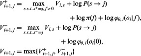That is, we optimize separately for the case of incorporation () and for the case of no incorporation (), taking the maximal value of the two.

In theory, one still needs to iterate over all possible value of f when computing . However, one can assume that all homopolymers are shorter than a certain length M. The Ion Torrent software sets M = 13. As the running time of the algorithm is linear in M, we chose an adaptive approach; we set a different value for each flow, given by . This reduces the value of M_i for most flows, thus greatly reducing the overall running time.

To obtain the maximum likelihood path, one only has to keep track of the values of s and f that are used to maximize each recurrence. We can then start with the optimal last state () and work our way backward using the standard dynamic programming backtracking procedure.

The running time of the algorithm is linear in n. The dynamic programming table contains n rows and columns. To compute the value of each cell, we must consider two values for s and M_i values for f. The backtracking algorithm is also linear in the size of the table. Therefore, the time complexity of the algorithm is O(nM), where . The space complexity is O(n), which is the size of the table.

3.3.1 Estimating the noise-model parameters

The likelihood of a set of noise model parameters θ can be calculated efficiently using the forward algorithm (Durbin et al., 1998); thus, the maximum likelihood estimators of the parameters can be used in the Viterbi. The forward algorithm is similar in spirit to the Viterbi algorithm. Given a value of the parameter set θ, we define as the likelihood of observing flows , given that the last state of the state machine is . The likelihood of the specific set of parameters θ is then given by .

A table is constructed in a similar manner to the Viterbi algorithm, with the major differences being using likelihoods instead of log likelihoods and summing over all previous states rather than using only the maximal previous state:

As in the case of the Viterbi algorithm, the specific state machine set-up enables faster computations by taking into account only possible state transitions and possible incorporation values.

As the likelihood of a set of parameters θ can be computed by the aforementioned forward algorithm, a reasonable approach would be finding the maximum likelihood estimator of θ and plugging it into the Viterbi algorithm. Although this approach is appealing, for every value of θ, the likelihood needs to be re-evaluated, resulting in a considerable increase in running time. We, therefore, suggest applying this procedure to a subset of flowgrams and use the mean value of θ as the parameter for the rest of the flowgrams. The maximization itself can be carried out using an exhaustive grid search. However, we found that using the greedy algorithm obtained similar results to the grid search (results not shown) while requiring only a fraction of the likelihood evaluations. Both methods are implemented in FlowgramFixer.

3.3.2 Relationship to a hidden Markov model

Finally, we wish to note the resemblance of our method to a hidden Markov model (HMM) technique (Baum and Petrie, 1966). In fact, our model can be expressed as an HMM by representing every consecutive pair of states as a single-hidden state and constructing transition and emission probabilities accordingly. However, we find the presentation via state machine to be more intuitive and straightforward.

4 RESULTS

We demonstrate our method using a publicly available dataset from Ion Torrent’s webpage, namely, C11-278. C11-278 is a re-sequencing experiment of E.coli DH10B, using the PGM with an Ion 318 chip.

We extracted the normalized and phase-corrected incorporation signals from the SFF files. The file contained 6 742 759 flowgrams and 1.65 Gb, respectively. The PGM was run using a wash cycle of 32 bases:

and used 520 flows. We note this is the default Ion Torrent wash cycle.

We first ran the default calling algorithm, which is equivalent to rounding the signals in the SFF file. We use this algorithm as a baseline for our comparisons. We then ran FlowgramFixer, which took ∼4 h on a single CPU (Xeon E7-8837 @ 2.67 GHz) with inconsequential memory use (<10 Mb). This run included a preliminary step of estimating the optimal noise-model parameters for a subset of 20 384 flowgrams, using a greedy algorithm, computing the mean intercept and trend and running the Viterbi on the entire dataset using the mean parameters. To ensure reproducibility, the subset of flowgrams we used originated from a 200-by-200 wells region from the chip, which were pre-specified by Ion Torrent and available on their website as an exploratory dataset. The mean intercept and trend were 0.0377 and , respectively.

The output of each algorithm is a list of integer-valued flowgrams, which we converted to reads and aligned to the reference with bowtie2 (Langmead and Salzberg, 2012) using default parameters.

First, we compared the number of uniquely aligned reads. The baseline rounding method yielded 3 537 723 uniquely mapped reads, whereas FlowgramFixer yielded 3 788 697—an increase of 250 974 reads (7.1%). Second, we counted how many reads (hard clipped at 200 bp) were mapped uniquely with high-mapping quality (Table 2). FlowgramFixer outperformed the baseline rounding method for all quality thresholds, with a 2.8–4.8% increase in the number of high-quality aligned reads.

Table 2.

Number of reads (hard clipped at 200 bp) mapping with quality above the given thresholds

Baseline	5 463 391	4 867 523	4 857 829
FlowgramFixer	5 617 599	5 098 930	5 088 117
Difference	154 208	231 407	230 288
Improvement (%)	2.8	4.8	4.7

Note: We used 20, 30 and 40 as thresholds, corresponding to mis-alignment probabilities of 0.01, 0.001 and 0.0001, respectively. FlowgramFixer is able to accurately map up to 4.8% more reads than the baseline.

We wanted to study the effect of the position along the wash cycle on error rates. For each flowgram corrected by the baseline method, we converted the aligned-to part of the reference genome to a flowgram and noted the flow positions that had a mismatch. We then averaged the error rates of flows that are identical (the length of the wash cycle) (Fig. 4). It is evident that different positions along the wash cycle display remarkably different error rates. This can partially be explained by patterns in the wash cycle. For example, positions 9–11 contain the nucleotides T, C and T. Because of the first T, the probability of observing incorporation at the second T is much lower; therefore, more flows have no incorporations. As no incorporations are easier to call, the error rate at the second T is much lower as well. A similar situation occurs at positions 25–27, containing T, G and T. Positions 11 and 27 are highlighted in red in Figure 4.

Fig. 4.

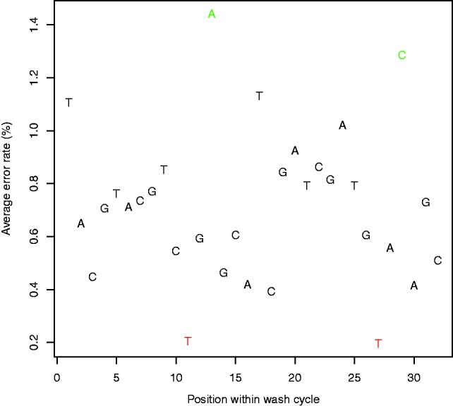
Dependence of error rate on wash cycle. Average error rates along the 32-nt long wash cycle, for the rounding method. The actual nucleotide in each flow is indicated by the corresponding letter. We used the first 320 flows to calculate the rates and discarded the first cycle to cancel the effect of the sequencing adapter. Note the high dependence of the error rate on the position in the wash cycle—positions 13 and 27 (colored red) display a considerably low error rate, whereas positions 11 and 29 (colored green) display a considerably high error rate. These changes in error rate can be partially explained by patterns in the wash cycle

The opposite effect can also be observed, such as the A at position 13. As there is a large gap between the appearance of the previous A (position 6), there is a higher probability of incorporation and, hence, of error. A similar situation occurs with the C at position 29. These positions are highlighted in green in Figure 4.

Next, we investigated the dependence of the error rate on the flow position. The average error-rates per flow of the rounding algorithm are portrayed in Figure 5. It is clear that the vast majority of errors occur at the ends of the flowgrams, and that such a high-error rate renders the ends of Ion Torrent reads useless. As this is the case for most, if not all, high-throughput sequencing technologies, most real-life applications involve a step of ‘clipping’—removing the 3′-end of each read—either by setting a pre-defined length (hard clipping) or using a reference genome to determine the optimal cut-off point (soft clipping).

Fig. 5.

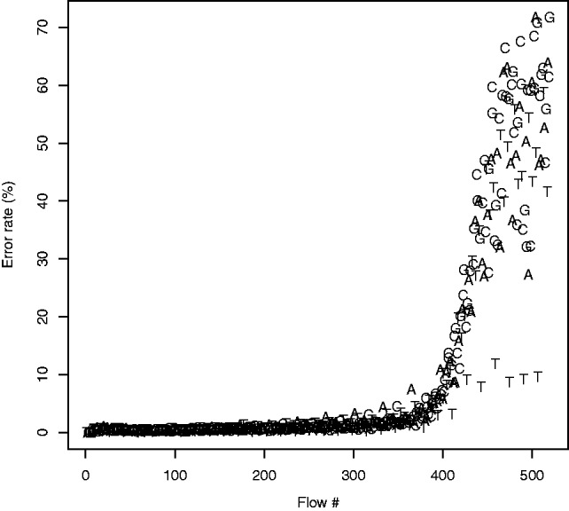
Per-flow error rates of the default calling algorithm used as a baseline for comparison. The error rate clearly increases with the flow number, with a dramatic increase beginning around flow 380

We, therefore, applied soft clipping to the 3′-end of each read using bowtie2 (using the local parameter) and re-estimated the per-flow error rates. The rounding algorithm had an average error rate of 0.88% per flow (Fig. 6). We note that this is probably the most common pipeline used in re-sequencing experiments. Running FlowgramFixer yielded an average error rate of 0.7%, a reduction of compared with the baseline. To test the robustness of this analysis to the choice of clipping method, we also tried hard clipping the reads at 200 and 300 nt. In these cases, FlowgramFixer reduced the error rate by 17 and 21%, respectively.

Fig. 6.

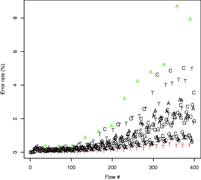
Per-flow error rates of the rounding algorithm, using soft clipping. As expected, the error rate increases as the sequencing process progresses, even after clipping. The dependency of the error rate on the position in the wash cycle is also evident. Similarly to Figure 4, flows that are 11th or 27th within a cycle (marked red) display a considerably lower error rate, whereas flows that are 13th within a cycle (marked green) display considerably higher error rates

We then compared the error rates of the two methods, per position (Fig. 7). Although the maximum obtained difference is as high as 3.4%, there are other positions where rounding actually does slightly better than FlowgramFixer. We believe that this may be because the variability in the noise at some positions of the wash cycle increases as the sequencing process progresses. We discuss possible solutions in Section 5.

Fig. 7.

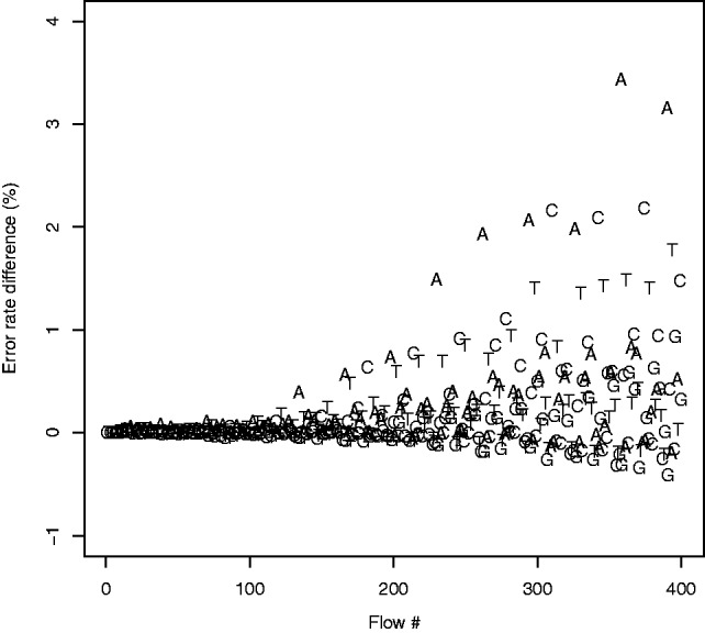
Error rate difference between the rounding method and FlowgramFixer (baseline error rate FlowgramFixer error rate). The average difference of error rate grows as the sequencing process progresses, as expected because of the noisier signal obtained at later flows. Although at some flows, the error rate decreases by as much as 3.4%, at other flows the error rate actually increases. Interestingly, the error rate difference also displays a dependency on the position in the wash cycle

5 DISCUSSION

We have focused on developing a general inference framework without making it overly reliant on the current intricacies of Ion Torrent’s platform. However, there are several possible extensions that, although making the approach less robust to technology changes, could improve its performance on today’s datasets. We discuss several such ideas later in the text.

Our noise model relies on a intercept and trend model for the standard deviation (SD) parameter. One might suggest richer models, including more complicated dependency of the SD on the flow index, dependency of the SD on the number of incorporated nucleotides and a dependency on the position along the basic 32-nt wash cycle. We briefly experimented with these ideas and were not able to find a richer model that improved the results while maintaining a reasonable running time. However, exploring these ideas further seems worthwhile. Additionally, we suggest that additional accuracy gains might be gained by adding a spatial structure to the noise model, as nearby wells experience similar artifacts during the sequencing process.

Our approach has the advantage that phase correction is done by Ion Torrent’s software before our analysis, thus reducing running times. However, one can think of combining the phasing and the calling algorithms into one probabilistic framework. Such a framework could help eliminate some of the artifacts introduced by the phasing algorithm and improve the quality of both the phasing and base-calling.

The use of smarter priors and better parameters can also improve the accuracy. Some Ion Torrent reads contain test fragments of pre-determined DNA sequence, which can be used to optimize parameter values, such as our θ. Furthermore, our maximum-likelihood framework allows for easy inclusion of priors on GC-content and homopolymer lengths. We suspect that incorporating an empirical Bayes before as in Quinlan et al. (2008) would increase the accuracy of our method. The impact of such priors would be greatest for genomes where the GC-content is different from 0.5, unlike E.coli.

The dynamic programming approach allows for other relevant extensions. For example, a forward–backward algorithm, similar to the forward algorithm, can be used to compute the marginal distributions of the flow values and derive statistically sound quality scores.

Finally, we note that our approach is embarrassingly parallelizable and low-memory. We, therefore, believe it could be run in a matter of minutes on a multi-core machine. Moreover, if incorporated into the Ion Torrent pipeline, it could be run ‘live’ as the sequencing process happens, making the running time inconsequential. In fact, the running time of our algorithm is similar to the running time of the subsequent alignment step; therefore, we believe that as long as the running time of our method remains reasonable, it should not be a bottleneck for end-users.

6 CONCLUSION

Although we are encouraged by the results of FlowgramFixer presented here, we recognize the quick pace at which technology evolves. As Ion Torrent continues to improve its sequencing technology (e.g. its new Ion Proton sequencing platform), it is likely that important parameters, such as the wash cycle, will evolve and the specific error profiles we observe today will evolve as well. However, we believe our major innovation—that inference should and could be done efficiently on the whole flowgram rather than flow-by-flow—will remain relevant for any future flowgram-based technology. Such technologies have been a major workhorse of the scientific community for several years, and it is likely they would remain relevant in upcoming years.

REFERENCES

- Balzer S, et al. Characteristics of 454 pyrosequencing data—enabling realistic simulation with flowsim. Bioinformatics. 2010;26:i420–i425. doi: 10.1093/bioinformatics/btq365. [DOI] [PMC free article] [PubMed] [Google Scholar]
- Baum L, Petrie T. Statistical inference for probabilistic functions of finite state markov chains. Ann. Math. Stat. 1966;37:1554–1563. [Google Scholar]
- Beuf K, et al. Improved base-calling and quality scores for 454 sequencing based on a Hurdle Poisson model. BMC Bioinformatics. 2012;13:303. doi: 10.1186/1471-2105-13-303. [DOI] [PMC free article] [PubMed] [Google Scholar]
- Durbin R, et al. Biological Sequence Analysis: Probabilistic Models of Proteins and Nucleic Acids. Cambridge, UK: Cambridge University Press; 1998. [Google Scholar]
- Eisenstein M. The battle for sequencing supremacy. Nat. Biotechnol. 2012;30:1023–1026. doi: 10.1038/nbt.2412. [DOI] [PubMed] [Google Scholar]
- Hopcroft JE, Ullman JD. Introduction to Automata Theory, Languages and Computation. Reading, MA, USA: Addison-Wesley; 1979. [Google Scholar]
- Langmead B, Salzberg SL. Fast gapped-read alignment with Bowtie 2. Nat. Methods. 2012;9:357–359. doi: 10.1038/nmeth.1923. [DOI] [PMC free article] [PubMed] [Google Scholar]
- Ledergerber C, Dessimoz C. Base-calling for next-generation sequencing platforms. Brief. Bioinform. 2011;12:489–497. doi: 10.1093/bib/bbq077. [DOI] [PMC free article] [PubMed] [Google Scholar]
- Lysholm F, et al. FAAST: flow-space assisted alignment search tool. BMC Bioinformatics. 2011;12:293. doi: 10.1186/1471-2105-12-293. [DOI] [PMC free article] [PubMed] [Google Scholar]
- Merriman B, et al. Progress in Ion Torrent semiconductor chip based sequencing. Electrophoresis. 2012;33:3397–3417. doi: 10.1002/elps.201200424. [DOI] [PubMed] [Google Scholar]
- Quail M, et al. A tale of three next generation sequencing platforms: comparison of Ion Torrent, Pacific Biosciences and Illumina MiSeq sequencers. BMC Genomics. 2012;13:341. doi: 10.1186/1471-2164-13-341. [DOI] [PMC free article] [PubMed] [Google Scholar]
- Quince C, et al. Removing noise from pyrosequenced amplicons. BMC Bioinformatics. 2011;12:38. doi: 10.1186/1471-2105-12-38. [DOI] [PMC free article] [PubMed] [Google Scholar]
- Quinlan AR, et al. Pyrobayes: an improved base caller for SNP discovery in pyrosequences. Nat. Methods. 2008;5:179–81. doi: 10.1038/nmeth.1172. [DOI] [PubMed] [Google Scholar]
- Rothberg JM, et al. An integrated semiconductor device enabling non-optical genome sequencing. Nature. 2011;275:348–352. doi: 10.1038/nature10242. [DOI] [PubMed] [Google Scholar]
- Vacic V, et al. Pacific Symposium on Biocomputing. 2008. A probabilistic model for small RNA flowgram matching; pp. 75–86. [PMC free article] [PubMed] [Google Scholar]