Minimum curvilinearity to enhance topological prediction of protein interactions by network embedding

Abstract

Motivation: Most functions within the cell emerge thanks to protein–protein interactions (PPIs), yet experimental determination of PPIs is both expensive and time-consuming. PPI networks present significant levels of noise and incompleteness. Predicting interactions using only PPI-network topology (topological prediction) is difficult but essential when prior biological knowledge is absent or unreliable.

Methods: Network embedding emphasizes the relations between network proteins embedded in a low-dimensional space, in which protein pairs that are closer to each other represent good candidate interactions. To achieve network denoising, which boosts prediction performance, we first applied minimum curvilinear embedding (MCE), and then adopted shortest path (SP) in the reduced space to assign likelihood scores to candidate interactions. Furthermore, we introduce (i) a new valid variation of MCE, named non-centred MCE (ncMCE); (ii) two automatic strategies for selecting the appropriate embedding dimension; and (iii) two new randomized procedures for evaluating predictions.

Results: We compared our method against several unsupervised and supervisedly tuned embedding approaches and node neighbourhood techniques. Despite its computational simplicity, ncMCE-SP was the overall leader, outperforming the current methods in topological link prediction.

Conclusion: Minimum curvilinearity is a valuable non-linear framework that we successfully applied to the embedding of protein networks for the unsupervised prediction of novel PPIs. The rationale for our approach is that biological and evolutionary information is imprinted in the non-linear patterns hidden behind the protein network topology, and can be exploited for predicting new protein links. The predicted PPIs represent good candidates for testing in high-throughput experiments or for exploitation in systems biology tools such as those used for network-based inference and prediction of disease-related functional modules.

Availability: https://sites.google.com/site/carlovittoriocannistraci/home

Contact: kalokagathos.agon@gmail.com or timothy.ravasi@kaust.edu.sa

Supplementary information: Supplementary data are available at Bioinformatics online.

1 INTRODUCTION

Detection of new interactions between proteins is central to modern biology. Its application in protein function prediction, drug delivery control and disease diagnosis has developed alongside a deeper understanding of the processes that occur within the cell. One key task in systems biology is the experimental detection of new protein–protein interactions (PPIs). However, such experiments are time consuming and expensive. Because of this, researchers have developed computational approaches for predicting novel interactions (You et al., 2010), intended also to guide wet lab experiments. The topological prediction of new interactions is a novel and useful option based exclusively on the structural information provided by the PPI network (PPIN) topology. This option for prediction is particularly convenient when the available biological information on the proteins being tested for interaction (seed proteins) is incomplete or unreliable. One of the most efficient approaches is the Functional Similarity Weight (FSW) (Chua et al., 2006). Such method belongs to the large and well-established family of predictors that are referred to as node neighbourhood techniques (Cannistraci et al., 2013a), because to assign a likelihood score to any candidate interaction (i.e. a pair of non-connected proteins in the observed PPIN), they rely on the topological properties of the seed proteins’ neighbours. The set of candidate interactions is then ranked. The main problem with these techniques is that their performance is poor when applied to sparse and noisy networks (You et al., 2010).

In 2009, Kuchaiev et al. (2009) proposed a method for geometric denoising of PPINs. The algorithm is based on the use of multidimensional scaling (MDS) to preserve the shortest paths (SP) between nodes in a low dimensional space. The predicted interactions are scored according to their Euclidean distance (ED) in the low dimensional space, following the principle that the closer two proteins are, the higher the likelihood that they interact (Kuchaiev et al., 2009). Although it is not explicitly mentioned in the article, the embedding method adopted by Kuchaiev et al. is equivalent to Isomap (Tenenbaum et al., 2000). In an independent study, You et al. (2010) proposed a hybrid strategy based on network embedding to assign prediction scores to candidate interactions. They exploited the notion that a PPIN—or theoretically, any network—lies on a low dimensional manifold shaped in a high-dimensional space. The shape of the manifold and the associated topology are determined by the constraints imposed on the protein interactions through biological evolution. You et al. used a renowned manifold-embedding algorithm, Isomap (Tenenbaum et al., 2000), to embed the PPIN in a space of reduced dimensionality. Then, they applied FSW to the embedded network (pruned according to a cut-off on the ED) to assign likelihood scores to the candidate interactions. In general, the embedding strategy offers two advantages: (i) the topological prediction performance is improved even when networks are sparse and noisy; and (ii) the computational time is reduced because the time required for the network embedding is much lower than that required by node neighbourhood techniques for computing the topological properties of each candidate interaction. A disadvantage is that if the network is not a unique connected component, only the largest connected component can be considered for embedding (Kuchaiev et al., 2009).

Here, we introduce several variations of these approaches that all together offer a new solution for topological link prediction by network embedding. The first variation uses minimum curvilinear embedding (MCE) (Cannistraci et al., 2010) and its non-centred variant, ncMCE (which is introduced for the first time), to project the network on the reduced dimensionality space. MCE is a parameter-free algorithm designed for the unsupervised exploration of high-dimensional datasets by non-linear dimension reduction (Cannistraci et al., 2010). Recently, MCE ranked first among 12 different approaches (evaluated on 10 diverse datasets) in a study on the stage prediction of embryonic stem cell differentiation from genome-wide expression data (Zagar et al., 2011). This proof of power and robustness motivated us to test its performance in the context of PPI prediction by network embedding. In the second variation, we use the SP distance (instead of the ED, as in Kuchaiev et al. and You et al.) over the network embedded in the reduced space to assign the likelihood scores to the candidate interactions. The method proposed here undoubtedly presents a novel combination of steps. We prove that the combination of ncMCE/MCE and SP achieves excellent results, boosting the separation between good and bad candidate links.

2 DATA AND ALGORITHMS

2.1 Network datasets

The main datasets analysed in this work comprise four yeast PPINs. Yeast networks are the preferred benchmark for testing topological algorithms to predict links because of the large amount of information available for yeast, in terms of both detected interactions and Gene Ontology (GO) associations (You et al., 2010). The PPIs in these datasets are mainly physical interactions, but also include literature-curated and functional links. Details on the characteristics of the networks are provided in Supplementary Section I and Table S1.

2.2 Network embedding algorithms

As this work focuses on link prediction based on network topology, each of the abovementioned datasets can be represented as an undirected unweighted graph with a set of nodes and a set of edges, which is a set of two-element subsets of . Network embedding consists of finding a mapping (embedding), , where is a set of points with : i.e. each node of is assigned a coordinate in a space of d dimensions, such that some original topological properties of the network are preserved in this low-dimensional space. As explained in the Introduction, manifold embedding algorithms can be easily adopted for network embedding, although not all algorithms that learn manifolds are applicable for this task: only those able to embed a topology starting from a distance or adjacency matrix can be used. We chose to compare MCE, ncMCE and Isomap (and Isomap + FSW) against well-established unsupervised and supervisedly tuned manifold embedding algorithms that accept a distance or adjacency matrix as input. The unsupervised embedding techniques considered are Sammon mapping (a type of non-linear MDS) (Sammon, 1969), and two force-based embedding techniques: stochastic neighbourhood embedding (SNE) (Hinton and Roweis, 2003) and tSNE (a variant of SNE) (van der Maaten and Hinton, 2008). The supervisedly tuned techniques are local MDS (Venna and Kaski, 2006) and neighbour retrieval visualiser (NeRV) (Venna et al., 2010). These methods are also force based, but instead of using forces based on kernels (like SNE or tSNE), they use forces based on neighbourhood graphs (Shieh et al., 2011). Both local MDS and NeRV require a parameter λ to be tuned between 0 and 1. In this work, we assessed the performance of these two techniques using values of λ from 0 to 1 in steps of 0.1, and took the low-dimensional coordinates that yielded the best prediction result (see Supplementary Sections II.2 and II.3).

2.3 MCE followed by shortest-path distance

MCE is a parameter free and time-efficient unsupervised algorithm for non-linear dimensionality reduction (Cannistraci et al., 2010), which was presented as a new form of non-linear MDS (see Algorithm 1 and Supplementary Section II.1 for details on the original version of MCE, the innovations proposed in this article and details on MCE’s time complexity). Here, we propose the use of MCE for embedding a network into a space of reduced dimensionality. MCE performs the embedding of the network connectivity distances measured over the minimum spanning tree (MST) of the original network. This novel MST-derived measure of connectivity was more generally formalized in a previous study as a non-linear measure that we refer to as minimum curvilinearity (MC), and the pairwise MC distances between nodes of the MST give rise to the MC matrix (Cannistraci et al., 2010).

The fact that the MST is a neighbourhood graph that can well approximate the main network information—offering a general summary of the network topology—has been extensively shown in different applications (Cannistraci et al., 2010; Shaw and Jebara, 2009; Shieh et al., 2011), and in our case, this can be particularly useful for denoising the information present in PPINs. In fact, the false-positive (FP) rate of currently widely used experimental technologies is significantly high, sometimes exceeding 60% (Kuchaiev et al., 2009).

MC tends to stress local topological distances and dilate large connectivity distances (Cannistraci et al., 2010). A consequence is that the use of MCE for embedding causes a sort of network deformation when the network structure is compressed in a reduced space of just a few dimensions. The deformation augments the separation between nodes far apart in the network topology and maintains or reduces the distances between nearby nodes (Cannistraci et al., 2010). This might be a point of weakness for network visualization because it stretches the network shape in the reduced space. However, it is a point of strength for link prediction because it generates a non-linear soft-threshold effect—a type of gradual denoising (Cannistraci et al., 2009) based on a non-linear transformation—on the network connectivity distances measured in the reduced space. The soft-threshold discriminates between candidate links of protein pairs far apart in the original network topology (which earn large score values because they are now connected by enlarged path distances in the embedded space), and candidate links connecting nearby proteins in the original network topology (which earn small score values because they maintain or reinforce their topological proximity in the embedded space).

To maximally exploit the effect of such soft-thresholding, we propose the use of the SP distance in the low-dimensional space. As the network topology—mapped to a reduced space—should now be sufficiently denoised by means of the MCE device, the use of the SP (instead of the ED) appears to be a more appropriate way to assign distances between nodes because it obeys the denoised network topology. This is even more reasonable considering that each interaction is remapped in the reduced space with a positive and definite numerical weight (see Supplementary Section II.1 and Fig. S2). In conclusion, we expect the SP to be a congruous measure for converting the topological discrimination obtained by the MCE soft-threshold effect into a value. This computational engagement between MCE as a technique for embedding (useful for denoising networks affected by FP interactions) and SP for determining network-connectivity distance (effective when the networks are pure or denoised, and present few FP interactions), gives rise to a synergy that can boost the separation between good and bad candidate links in the ranking.

2.4 Non-centred MCE

The expression crowding problem means that after dimension reduction, data clusters collapse on top of each other in the reduced embedding space (van der Maaten and Hinton, 2008). This problem has particular relevance in network embedding because we want to avoid diverse network components collapsing in the same region of the reduced space, as this can cause incorrect link predictions. For this reason, we decided to introduce the ncMCE and test its performance in solving the crowding problem.

Here, we propose a new version of MCE as an inedited form of non-linear-kernel principal component analysis. In this new version, the MC matrix is interpreted as a non-linear and parameter-free kernel, and MC is a non-linear and parameter-free measure that produces a distance transformation stored in the MC kernel (previously referred to as the MC matrix). The first step of the new algorithm remains unaltered, while the embedding of the MC kernel is now executed by singular value decomposition (SVD) according to the following procedure: (i) centring of the MC kernel; and (ii) SVD decomposition of the centred MC kernel, followed by the embedding in an arbitrary dimension. An advantage of the new algorithm is that the centring of the MC kernel can be omitted (see Algorithm 1 and Supplementary Fig. S1). In practice, this generates a different dimension-reduction device, which we refer to as non-centred MCE (ncMCE). There is no universal rule for when centring transformation should be used in the analysis. Nevertheless, non-centring has been shown to offer several advantages (Basnet, 1993; Jolliffe, 2002). This is particularly evident in visualization tasks, when the set of points that form each cluster is distributed around the centre of the mass in the high-dimensional space. If we perform embedding in two dimensions after the centring transformation, the points tend to overlap around the origin of the first two dimensions, which is a typical example of the crowding problem. However, in most cases, executing the embedding without centring can significantly reduce this issue. In addition, omission of the MC kernel centring means that ncMCE has a time complexity of , and thus is more efficient than the other considered embedding techniques, such as MCE and Isomap, that have a time complexity of . For this reason, ncMCE also offers a significant computational advantage for handling very large networks (see Supplementary Section II.1.2 and Table S2).

The new algorithm for ncMCE and MCE is available on the website indicated in the abstract.

Algorithm 1 Minimum Curvilinear Embedding (MCE).

Input:

  , adjacency matrix representation of a PPIN (n = number of nodes in the network);

  , the embedding dimension;

  , a Boolean specifying whether the MC kernel will be centred or not;

Output:

  , matrix whose rows are the points with coordinates in a -dimensional reduced space;

Description:

  Extract the minimum spanning tree out of ;

  Compute the distances between all node pairs over to obtain the MC kernel ;

  If TRUE: Centre kernel , i.e. with ;

  Else: Continue;

  Perform ‘economy size’ singular value decomposition of ;

  Return ;

* indicates matrix transpose, is the identity matrix and 1 is a column vector of ones.

2.5 Node neighbourhood methods

To assess interaction reliability, several node neighbourhood techniques for link prediction have been proposed to exploit the topology of a PPIN, such as Interaction Generality (IG1) (Saito et al., 2002), IG2 (Saito et al., 2003) and IRAP (Chen et al., 2005), or to predict protein function, such as the Czekanowski-Dice Dissimilarity (CDD) (Brun et al., 2003) and FSW (Chua et al., 2006). These techniques have also been used to predict PPIs based on the topological properties of the neighbours of candidate protein pairs (You et al., 2010). As shown in Chen et al. (2006) and Chua et al. (2006) and mentioned in You et al. (2010), FSW and CDD outperform IG1, IG2 and IRAP. Because of this evidence, and considering that IG2 and IRAP are very computationally expensive (Chen et al., 2005), we decided to use only IG1 (as a baseline), CDD and FSW (details and associated formulae for these approaches appear in Supplementary Section III).

3 METHODS

3.1 Testing the proposed innovations

3.1.1 Fraction of FPs visited by MC and SP

We generated 1000 random geometric graphs (for details see section 3.1.4) with small-world and scale-free topology, which are properties common to real biological and PPI networks. Each network had 1000 nodes and was modelled with levels of noise similar to those of real PPINs: around 40% false negatives (FNs) and 60% FPs (Kuchaiev et al., 2009). We counted the fraction of unique FPs visited out of the total number of FPs present when computing SPs between all node pairs over the entire network (first step of the Isomap algorithm) and over the MST (first step of the MCE algorithm).

3.1.2 Solving the crowding problem

Although it is not a biological dataset, the radar signal dataset is a point of reference in machine learning and is an important benchmark for testing the ability of embedding techniques to solve the crowding problem (Shieh et al., 2011). Instead of creating an artificial dataset, we decided to use a real one to test whether ncMCE is able to solve the crowding problem and, as a result, better embed networks into low dimensions. The radar signal dataset is highly non-linear and has 351 samples characterized by two classes: good radar signals that are highly similar, and bad radar signals that are highly dissimilar (Shieh et al., 2011).

3.1.3 Discrimination between good and bad candidate links

Following Kuchaiev et al. (2009) and You et al. (2010), for each of the four considered yeast networks, we fitted a non-parametric estimate to the distribution of low-dimensional distances between connected nodes in the network and another one to the distribution of distances between non-adjacent nodes . We used the Mann–Whitney non-parametric test to determine whether there was a statistically significant difference between and 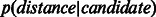over the different dimensions of embedding.

3.1.4 Evaluation on random geometric graphs

Random geometric graphs (RGGs) are important because there is indication that they can be good models for networks such as PPINs (Przulj et al., 2004). We generated RGGs by accommodating 1000 points uniformly at random in the 100-dimensional unitary cube and then connected them if and only if the dot product (similarity) between the vectors with tails in the origin and heads over these points was above a connectivity threshold r. We set the threshold by ensuring that properties common to real biological networks (small-world and scale-free topologies) and connectivity were present. The advantage of using RGGs to test our innovations is that the sets of true and spurious interactions are clearly defined: true interactions are those that fulfil the threshold and spurious links are those that do not. Based on this, we generated noise in the structure of 1000 different RGGs (noisy networks) in amounts typical of PPINs (40% FNs and 60% FPs) and performed a sparsification experiment in which the embedding predictors (a detailed explanation of how embedding prediction works is given in section 3.2 and Fig. 1) were adopted to rediscover the removed true interactions present in the generated RGG. During this test, the networks were embedded into dimensions 1 to 10, which is the recommended range for testing the performance of Isomap (You et al., 2010). Next, we repeated the experiment to assess the performance of the embedding predictors on a sparsification experiment over 1000 different RGGs without noise (clean networks).

Fig. 1.

Link prediction and performance evaluation in PPINs. The components in red correspond to the novel features proposed in this study

3.2 General prediction and GO-based evaluation framework

The flow diagram in Figure 1 depicts the required steps for link prediction and GO-based performance evaluation in PPINs. In the prediction phase, the original network lying in the high-dimensional space is represented as an adjacency matrix with entries if nodes and interact and otherwise (each of these non-adjacent pairs of nodes is considered a candidate interaction). Next, the network is embedded into a reduced space (initially of dimension 1) where both the original network links and the candidate edges are scored by means of either ED (as in Kuchaiev et al. and You et al.) or SP (our proposed variation, see section 2.3). Both sets of links are then ranked (see table of scored interactions in Fig. 1). A criterion (based on the ranked list) is used to automatically determine an appropriate dimension into which the network should be embedded (see sections 3.3 and 4). If the criterion is not fulfilled, the above procedure is repeated for a higher dimension, otherwise it stops and a list is output using only the ranked candidate interactions (see table of scored candidate interactions in Fig. 1). The code that takes as input and provides the scored list of candidates as the output is available on the website provided in the abstract.

The evaluation phase is specific to PPINs and follows the same gene ontology (GO) strategy adopted in past studies (Chen et al., 2005, 2006; Saito et al., 2002, 2003; You et al., 2010). The proteins involved in the interactions from the candidate list are annotated via GO terms (molecular function or MF, biological process or BP, and cellular compartment or CC). If the terms associated with a protein pair have a high Wang’s GO semantic similarity (see Supplementary Section IV.2), the PPI is considered to be biologically relevant (marked with a Yes in the table in Fig. 1) and is used to quantify the precision of the predictors. GO is used to assess how precisely the prediction techniques place candidate interactions that are likely to be real at the top of the ranking list (You et al., 2010). A recursive procedure is applied to create a precision curve. Each time, an increasing fraction of candidate PPIs (the first 100, the first 200 and so on) is taken from the top of the list of ranked candidate interactions for consideration. The fraction of candidate interactions that are relevant to GO generates a point on a precision curve. Conventionally, a number of top-ranked candidate links, equivalent to 10% of the links in the original network, is used to compute the entire precision curve (You et al., 2010). We also examine the curve generated for a number of candidates equal to 100% of the original network links (see Supplementary Section IV). The area under the precision curve (AUP)—normalized with respect to the x-axis so that it ranges from 0 to 1—summarizes the performance of the prediction technique for a given network. Precision and AUP are the preferred statistics (Chen et al., 2005, 2006; Saito et al., 2002, 2003; You et al., 2010) for evaluating the predicted links in biological networks, owing to their noisy nature. Having a non-adjacent pair of proteins in PPINs does not mean they cannot interact at all, and we cannot label the missing interaction as a TN. It is quite possible that these proteins have not yet been tested for interaction, or that it is experimentally difficult to do so (see Supplementary Section IV). As a result, performance statistics that do not rely on the number of TNs, such as Precision, are more suitable in this context than others, such as the AUC.

We also propose an innovative strategy for evaluating the performance of a link prediction technique at different levels of random sparsification of the original PPIN. Given a network , we generated an initial set of 50 sparsified networks by removing a fixed portion of links (10% of links) uniformly at random from the original topology (sparsification process). Then, we generated a second set of 50 sparsified networks by removing the same fixed amount of links, , uniformly at random from the networks sparsified in the previous step (a total of 20% of links removed). This process was repeated several times up to the point where network connectivity was lost. The AUP of each prediction technique was computed for each percentage (proportion of links removed) for the 50 networks, and the average AUP is reported as a sparsification curve. In addition, the area under this sparsification curve is useful for quantifying the robustness of a technique as a function of the network sparsity, which is one of the main issues for current link predictors (You et al., 2010).

Some GO annotations may be subject to experimental bias or come from not very reliable sources (Rhee et al., 2008). To address this issue, and as an additional verification of the candidate interactions proposed by the best techniques, we performed what we call an in-silico validation. We took the top 100 candidate interactions proposed by the best techniques and intersected them with the entire STRING Database (Szklarczyk et al., 2011) in March 2013. STRING is the most complete compendium of PPIs found in the literature, experiments, coexpression, etc. Given a list of proteins, it finds the interactions between them along with an assigned confidence value based on the available evidence that they exist. The output of this validation was used to compute (i) the number of protein pairs validated for each network out of the top 100; (ii) the average STRING confidence along with its standard deviation; and (iii) the average GO confidence along with its standard deviation. Note that this validation was carried out for candidate interactions only, and the PPIs of the used main network datasets were not considered in this analysis. Therefore, the overlap between the studied networks and STRING is unlikely to influence the results (see Supplementary Section I).

3.3 The AUC criterion for dimension determination

The AUC criterion is designed to work in combination with any network embedding algorithm adopted for link prediction: it automatically determines the dimension into which the network should be embedded (see Supplementary Section II.4.1 for details). For a certain dimension of embedding, the prediction procedure (Fig. 1) assigns a likelihood score to each interaction (low scores correspond to interactions that are likely to occur and high scores to interactions that are not). The scores are computed for both the original interactions in the network (O) and the candidate interactions (C), which are all those protein pairs that were not linked in the input network.

The scored O and C interactions generate two distance distributions (see Supplementary Fig. S7 for an example). As suggested by Kuchaiev, You and their teams, we can vary a cut-off ε, from 0 up to the maximum distance of the two distributions, so that all protein pairs with scores below ε are considered positives and all protein pairs with scores above ε are considered negatives (Supplementary Fig. S7). Kuchaiev et al. and You et al. suggest that by taking the original network PPIs as our positive set, we can compute the number of TPs, FNs, FPs and TNs at each ε cut. This will yield a pair (1-Specificity, Sensitivity) that, measured for the entire ε range, generates a Receiver Operating Characteristic curve (ROC) and an Area Under the ROC Curve (AUC) that characterizes the performance for the current dimension (Supplementary Fig. S7). Both research groups showed that the AUCs for different dimensions were very similar and the increase in the AUC value tended to vanish for higher dimensions; thus, they considered a fixed dimension of 5 and 10 respectively for their experiments (You et al., 2010). We took advantage of this finding (Supplementary Fig. S7) by computing the AUC for each dimension, starting with dimension 1 and continuing until the difference between the AUC of one dimension and the next was less than 1E-3. In several tests, we found that 1E-3 represents such a small difference between AUCs that we can consider it not significant; thus, the last AUC is considered appropriate to identify the dimension for embedding. We then took the scored candidate interactions given by this dimension for the final evaluation of the method used.

3.4 The resolution criterion for dimension determination

One of the motivations for proposing a second criterion was that the AUC criterion considers the original network as a sort of gold standard, when in reality it includes several false interactions (You et al., 2010). The new criterion for dimension determination is based on the idea that the greater the difference between likelihood score values, the better they discriminate between good candidates and bad candidates in the ranking. Thus, we need to define a measure of the resolution of the score values provided by each dimension, such that the higher the measure, the higher the resolution and the more we should consider this dimension as correct for embedding. The measure we use for dimension determination is as follows:

(1)

This formula takes all of the unique score values of the candidate interactions in dimension Dim, computes its standard deviation σ and divides it by Dim. The unique score values give us an indication of the Dim’s resolution. We then determine the quality of that resolution by computing σ, which quantifies the variation between the unique score values. Finally, the division by Dim penalizes the higher dimensions, which have been shown not to provide any relevant increase in performance (You et al., 2010). We specifically designed this criterion to fit with the quality of MCE, which provides more of a soft-threshold effect in low dimensions. This is why we only tested the resolution criterion in combination with MCE. We also applied a variation of Equation (1) to check whether dimension determination using only the ranked interactions between 0 and 100 would generate a better AUP. The difference between Equation (1) and (2) is that in (2) we compute σ on the unique scores from the top 100 candidate protein pairs:

(2)

4 RESULTS AND DISCUSSION

4.1 Fraction of FPs visited by MC and SP

The results presented in Supplementary Figure S3 for the artificial networks (RGGs) suggests that the estimate of non-linear connectivity measure using the MST (i.e. MC) takes into account only a small proportion of FPs, offering a denoised estimate of the network connectivity. In contrast, using the SP over the entire noisy network counts all FPs at least once, which introduces a lot of noise into the link prediction process. The same investigation was conducted on the four yeast networks, in which the FP links were identified using the same GO-based strategy mentioned in section 3.2. The outcome of this second analysis (Supplementary Fig. S3) converged to the same result obtained for the artificial networks. These findings support the hypothesis that MCE should be a powerful tool for link prediction in noisy networks. In fact, as noisier networks present more FP interactions, the use of ncMCE/MCE in such cases should produce an even greater increase in performance over the use of Isomap. As current PPINs are sparse and noisy (You et al., 2010), the use of ncMCE/MCE instead of Isomap should offer clear advantages in network denoising and link prediction in the reduced space. A proof of this is provided in the computational experiment on RGGs discussed in section 4.4.

4.2 Solving the crowding problem

The ncMCE (Fig. 2A) offered the best embedding of the radar signal dataset and attained high linearization (Fig. 2E) in both the first (AUC = 0.95) and the second dimensions (AUC = 0.96). The ROC curve is used to evaluate the discrimination power along a dimension of projection: if the dimension offers a linear discrimination between the good and bad signals, the respective AUC will be 1. We also tested the performance of Isomap, which is a reference algorithm for non-linear dimension reduction, but its embedding was highly crowded (Fig. 2C).

Fig. 2.

Embedding of the radar signal dataset. The red spots indicate good radar signals. The grey and black spots indicate bad radar signals, which might be interpreted as two diverse sub-categories of bad signals. (A) ncMCE. (B) MCE. (C) Isomap. (D) TPE. (E) ROC and respective AUC computed for evaluating the linear discrimination performance of the first (Dim1) and second (Dim2) dimensions. The evaluation was repeated for each of the four techniques on the two dimensions of embedding. To facilitate the visualization, we do not report the ROC for TPE due to its poor performance

In contrast, Tree Preserving Embedding (TPE) (Shieh et al., 2011)—a recent parameter-free algorithm for non-linear dimension reduction—produced non-linear discrimination (good signals in the centre and bad signals on the periphery) of the clusters around the origin of the axis (Fig. 2D). This demonstrates that TPE can address the crowding problem but cannot solve the non-linearity of the dataset. MCE solved the non-linearity in the second dimension (Fig. 2E), but only partially addressed the crowding problem (Fig. 2B). The only algorithm that was able to simultaneously solve both the non-linearity and the crowding problem in this dataset was ncMCE (Fig. 2A and E). Interestingly, on the basis of the embedding offered by ncMCE and MCE, one might speculate that the high dissimilarity between the bad radar signals pointed out in previous studies (Shieh et al., 2011) could be interpreted as the presence of at least two different kinds of bad radar signal clusters that are difficult to embed due to their high non-linearity (elongated and/or irregular high-dimensional structure). The possible different bad-signal clusters are indicated in grey and black in Figure 2. Finally, whereas only a few seconds were needed to run ncMCE, MCE and Isomap, TPE took several hours to embed this small dataset, and its current implementation can be prohibitively slow for large datasets. As TPE is inefficient for embedding networks composed of thousands of nodes, we could not evaluate its performance in the present study.

4.3 Discrimination between good and bad candidate links

Given the embedding of any PPIN, if the hypothesis that nodes closer to each other in the reduced space are more likely to interact is true, the network-link distribution should have higher peakedness (kurtosis) than the candidate-link distribution ; in addition, original) should be shifted towards zero. The results in Figure 3 and Supplementary Figure S4 show that in all networks, ncMCE-SP had the highest kurtosis and shift towards zero. Moreover, links from the original network topology that are distant from the origin are likely to represent false positives, while non-adjacent nodes whose distance is close to zero are good candidates for interaction.

Fig. 3.

Discrimination between original network and candidate PPIs. Distribution of shortest-path scores in the reduced space (dimension 3 displayed) for Ben-Hur and Noble 2005 dataset. Network links p(distance|original) (solid line) and candidate links p(distance|candidate) (dashed line) after (A) ncMCE and (B) Isomap network embedding. The insets show the distribution of Euclidean distance scores

Furthermore, Supplementary Figure S4 shows that in the four considered networks, there was a statistically significant difference between 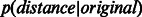and . This significant difference was conserved across the different dimensions, and was much larger when the SP scoring technique was used in the reduced space. This indicates that SP should work better than ED for scoring proximity distances between network nodes (proteins) in the reduced space.

4.4 Evaluation on random geometric graphs

Figure 4A–C shows that the two variations of MCE (especially ncMCE-SP using dimension one) were the strongest approaches for re-predicting true interactions in 1000 RGGs with similar levels of noise to those in real protein networks. Next, Figure 4D–F shows that when we repeated this experiment in 1000 RGGs without noise, ncMCE-SP still had the best performance (using dimension 1), but Isomap-SP came significantly closer. However, as our RGGs are sparse, the number of candidate links is very large compared with the number of links deleted during sparsification. In such conditions, link prediction is generally a difficult task, and this justifies the low precision values in Figure 4 (see Supplementary Section II.1.1 for more details). Altogether, these results indicate that (i) the use of ncMCE presents a clear advantage over MCE; (ii) the lower dimensions (especially dimension 1 for ncMCE) are very effective when using ncMCE/MCE-based algorithms; (iii) the gap between ncMCE-SP and Isomap-SP increases in the presence of noise, which especially encourages the use of ncMCE-based algorithms in noisy networks such as PPINs; and (iv) the use of SP (to assess the scoring in the reduced space) generally offers a clear advantage over the use of ED. RGGs are crucial for designing a ground-truth evaluation that allows us to directly observe the effect of introducing noise (false interactions) in the re-prediction of the real/original network topology. Because GO-free evaluations are essential for demonstrating the performance of link predictors in the absence and presence of network noise, the findings here are our first important results.

Fig. 4.

Sparsification and reprediction of random geometric graphs. Mean re-prediction precision of true-positive interactions for different sparsification levels of noisy networks with 60% false-positive interactions in their original topology: embedding dimensions 1 (A) and 4 (B) are displayed. The standard error bar is reported for each point. Analogous plots for clean networks (which do not present false-positive interactions in their original topology) are reported again for dimensions 1 (D) and 4 (E). The Area under the Mean Precision Curve is reported for each dimension of embedding, considering the re-prediction of true-positive interactions in noisy (C) and clean (F) networks. The arrow indicates the overall best performance (given by ncMCE-SP in dimension one). The percentage improvement in respect to the best Isomap (ISO-SP) performance is reported

4.5 Evaluation using gene ontology

The novel approach we propose is based on the intuition that network embedding by ncMCE/MCE combined with the SP connectivity distance in the reduced space can boost the performance in topological prediction of candidate PPIs. In Figure 5, we provide experimental confirmation of our intuition (see Supplementary Figs S11, S12 and S13, where we show that even when the Molecular Function GO category is excluded, when a wider candidate list of interactions is included in the evaluation or when proteins involved in large complexes are removed from the analysis, in general, our proposed approaches outperform the others). MCE and ncMCE combined with SP outperformed both Isomap and pure SP (computed on the original network without embedding) in all networks. Isomap performed even worse than pure SP in the first network. Besides, the simulation in Figure 5 suggests that in general ncMCE-SP slightly outperforms MCE-SP; and Supplementary Figure S6 shows that ncMCE-SP even outperfomed Isomap + FSW.

Fig. 5.

Performance comparison between ncMCE, MCE, Isomap and pure SP computed in the high-dimensional space. The x-axis indicates how many interactions are taken from the top of the candidate interaction list (sorted decreasingly by score), and the y-axis indicates the precision of the technique for that portion of protein pairs. Solid lines indicate the use of the SP in the reduced space to assign scores and dashed lines the use of the ED

In addition to the above results, there is evidence (Fig. 6) that although we used several advanced techniques for dimensionality reduction (both unsupervised and supervisedly tuned), ncMCE-SP remained the overall leader, which represents our second important finding. Surprisingly, we discovered that even though local MDS and NeRV were supervisedly tuned to achieve their best performance, they could not equal ncMCE-SP. This result suggests that force-based methods for embedding are not appropriate in this context, at least when combined with ED or SP in the reduced space. The reason for their poor performance is that these algorithms perform an embedding that finely preserves the network topology, thus also preserving the noise. In contrast, ncMCE provides a soft-threshold effect (discussed in Section 2.3), which boosts the separation between good and bad candidate links in the ranking.

Fig. 6.

ncMCE-SP against advanced unsupervised and supervisedly tuned embedding techniques. The x-axis indicates how many interactions are taken from the top of the candidate interaction list (sorted by decreasing score), and the y-axis indicates the precision of the technique for that portion of protein pairs. Solid lines represent the performance of techniques that use SP in the reduced space to assign scores and dashed lines represent techniques that use ED. Although ncMCE-SP (red solid line) is an unsupervised approach, it appears on both sides for reference

For completeness, we compared ncMCE-SP with FSW and CDD, two of the most efficient node neighbourhood techniques (You et al., 2010). ncMCE-SP ranked first, with a notable improvement, in the first two networks (Ben-Hur and Noble 2005; Chen et al. 2006; Supplementary Fig. S9), and second in the third network (You et al. 2010 sparse, Supplementary Fig. S9). In the fourth network, all of the techniques produced similar performances (You et al. 2010 dense, Supplementary Fig. S9). According to the minimum precision curve attained in the four different networks, ncMCE-SP was also the most robust technique (Robustness comparison, Supplementary Fig. S9). FSW ranked first in the third network, while in the first two networks its performance was similar to that of CDD. Given these results, we can conclude that ncMCE-SP offers a general improvement, particularly in robustness, compared with the other techniques.

4.6 Testing the criteria for dimension determination

Another important variation we introduce here is the use of two diverse criteria for automatically selecting the congruous dimension into which the network should be embedded. So far, in the simulation showed in Figures 5 and 6, we used the AUC criterion, which was designed to work with any algorithm for embedding. Unlike the AUC criterion, the resolution criterion was designed to fit better with MCE, which provides more of a soft-threshold effect (thus stronger denoising) in the lowest dimensions.

This is experimentally confirmed in Supplementary Figure S8A, where the peaks of the resolution criteria (both Res_All and Res₁₀₀) are always in one of the first two reduced dimensions. From Supplementary Figure S8B, we gather that the AUC criterion and the Res_All criterion selected the same dimensions, and thus show equal precisions. However, in terms of robustness (Supplementary Fig. S8C), the Res₁₀₀ criterion slightly outperformed the others. These results corroborate our intuition to invent a new and radically different criterion based on the resolution of the unique score values, which is an easy and time-efficient strategy.

4.7 Network sparsification evaluation

To present a more refined vision of the potential offered by topological link-prediction techniques, we introduce a new evaluation strategy called network sparsification experiment (see section 3.2 for details). This approach was used to generate the results shown in Figure 7, which compares the main embedding techniques (ncMCE, MCE and Isomap) and the reference node neighbourhood techniques (FWS, CDD, IG1 and SP). All of the embedding methods were tested in combination with the same distance (SP) to measure candidate-link likelihood in the reduced space. Figure 7A and B display the sparsification curves of the first two networks for ncMCE-R (R indicates the use of the resolution criterion) and FSW that were the highest ranked methods overall in their respective categories. Although ncMCE-A (A indicates the use of the AUC criterion) attained the same result as ncMCE-R in each network, for the sake of clarity, we display only the curve of the latter. The methods were ranked considering the area under the sparsification curve (AUS). To evaluate the general performance of the methods, we considered the minimum AUS performance of each method for all networks (Fig. 7C).

Fig. 7.

Network sparsification and redensification. (A and B) Sparsification curves (solid line) and redensification curves (dashed line). The arrows indicate the direction of the simulation (right for sparsification and left for redensification) as a function of the average node degree. Each point on the curves is obtained as the average AUP on 50 random sparsified or redensified networks, and the standard error bar is reported. (C) Sparsification robustness is useful for quantifying the robustness of a technique as a function of the network sparsity. It is computed as the minimum area under the sparsification curve (AUS) among all networks. The red bins indicate MCE-based methods; the green bins indicate neighbourhood-based methods; the blue bins indicate Isomap-based methods; and the violet bin indicates the pure SP directly applied on the network

A special variation of this experiment was performed on each network (Supplementary Fig. S5) to investigate whether the extraction of different MSTs from the networks resulted in important changes in ncMCE performance. This is a possibility because all of the network links have a weighting value of 1. For this test, only ncMCE was used because it generally outperformed MCE, as shown in Figures 5 and 6. Here, for each percentage of link deletions, 100 different MSTs were extracted (by random initialization). The AUPs attained by the different ncMCEs (each of which uses a different MST) were averaged and their standard error bars included in the sparsification curve. The standard error bars for the ncMCE’s sparsification curves (Supplementary Fig. S5) show that the difference in the performance of ncMCE when using different MSTs was negligible.

In general, MCE-based embedding techniques (red bins in the histogram, Fig. 7C) outperformed the node neighbourhood techniques (green bins in the histogram, Fig. 7C), and ncMCE was again the best method. Taken together, our experiments suggest that ncMCE-SP might represent a new benchmark for robustness in the topological prediction of PPIs, and this is the third main result of our study.

As a further investigation, starting with the final set of sparsified networks generated in the previous experiment, we re-densified their topologies by random addition of links and applied two approaches (ncMCE-R and FSW) at each percentage of densification. As we can see in Figure 7A and B, this process was unable to re-create a meaningful topology that might have been shaped by evolutionary features in the history of the protein interactome. If a topology analogous to the original had been recovered, the prediction techniques would have been able to achieve a performance comparable with that reached before network sparsification.

This finding emphasises the presence of preferential bio-information in the PPIN topology that cannot be modelled by uniform random sampling of new interactions. Therefore, the simple unweighted topology can be highly informative for different purposes, one of them being the prediction of new interactions or alternatively, as recently shown, the structural controllability of any complex network (Liu et al., 2011).

4.8 In silico validation

As mentioned in the Introduction, the experimental detection of PPIs can be very expensive in terms of both time and money. The computational approaches we investigated to predict novel interactions are meant to guide wet-lab experiments rather than to complete the interactome of the organism under study. Currently, the Y2H validation of 100 protein pairs can represent a challenging upper limit to simulate a real scenario for the budget of many labs. We decided to suggest different sets of candidate interactions to test in wet-lab experiments, and we report the evaluations for different thresholds: 20, 40, 60, 80 and 100. We executed an in-silico validation to verify the quality of the candidate interactions proposed by the best techniques. The top 100 ranked interactions for ncMCE-SP-Res₁₀₀ and FSW were tested on the STRING database, which is the most complete PPI database. The results for the different thresholds are reported in Supplementary Figure S10E. ncMCE-SP-Res₁₀₀ attained promising results in this last test, surpassing FSW for GO precision (Supplementary Fig. S10A and D), GO robustness (Supplementary Fig. S10B) and STRING confidence robustness (Supplementary Fig. S10C and D).

The list of the top 100 candidate interactions ranked by ncMCE-SP-Res₁₀₀ is reported for each of the analysed networks in Supplementary Table S1 and the respective list for FSW in Supplementary Table S2. GO semantic similarities and STRING confidence values are also included. To search for the biological information related to the interactions predicted by ncMCE-SP-Res₁₀₀ and validated in STRING, for each network we performed a pathway enrichment analysis using DAVID Bioinformatics Resources 6.7 (Huang da et al., 2009a, b). For each network, the list of proteins involved in the predicted and validated interactions was tested against all network proteins as background. This kind of background choice was motivated by the fact that it tends to produce more conservative P-values and, in fact, a general guideline for the enrichment analysis is to use a narrowed-down list of genes instead of all genes in the genome (Huang da et al., 2009a, b). In addition, the Benjamini correction for multiple hypotheses test was applied. The results of the analysis (reported in Supplementary Table S3) emphasize that the lists of predicted and STRING-validated protein interactions have significant biological meaning in at least one pathway for each of the investigated networks. Interestingly, the predicted proteins were involved in cellular processes (e.g. cell cycle), nucleotide metabolism (e.g. pyrimidine and purine metabolism) and genetic information processes (e.g. RNA polymerase and RNA degradation). This evidence suggests that the proposed method predicted interactions in different network modules that are related to significant and heterogeneous pathways in yeast.

5 CONCLUSIONS AND PERSPECTIVE

Considering the difficulty of dealing with sparse and noisy protein networks (You et al., 2010), our results represent a promising achievement and encouragement to further the investigation of network embedding techniques for topological prediction of candidate protein interactions. In our tests, the ncMCE showed enhanced performance in network embedding-based link prediction compared with the other dimension-reduction algorithms. In addition, ncMCE has a time complexity of only —which is lower than the complexity of the other considered machine learning techniques—and is a valid candidate for handling very large networks. Finally, our experiments revealed that the shortest path works significantly better than the Euclidean distance for scoring proximity distances between network nodes (proteins) embedded in the reduced space. We envision that network-embedding techniques for predicting novel PPIs might play an important role in the development of systems biology tools, such as those used for network-based inference of disease-related functional modules and pathways (Cannistraci et al., 2013b). The real biological interactions could be complemented with the in-silico predicted ones to boost the inference of the functional modules. In the near future, this last point will become increasingly important for patient classification, diagnosis of disease progression and planning of therapeutic approaches in personalized medicine (Ammirati et al., 2012).

REFERENCES

- Ammirati E, et al. Identification and predictive value of interleukin-6+ interleukin-10+ and interleukin-6- interleukin-10+ cytokine patterns in ST-elevation acute myocardial infarction. Circ. Res. 2012;111:1336–1348. doi: 10.1161/CIRCRESAHA.111.262477. [DOI] [PubMed] [Google Scholar]
- Basnet K. Centering of data in principal component analysis in ecological ordination. Tribhuvan Univ. J. 1993;16:29–34. [Google Scholar]
- Ben-Hur A, Noble WS. Kernel methods for predicting protein-protein interactions. Bioinformatics. 2005;21:i38–i46. doi: 10.1093/bioinformatics/bti1016. [DOI] [PubMed] [Google Scholar]
- Brun C, et al. Functional classification of proteins for the prediction of cellular function from a protein-protein interaction network. Genome Biol. 2003;5:R6–R6. doi: 10.1186/gb-2003-5-1-r6. [DOI] [PMC free article] [PubMed] [Google Scholar]
- Cannistraci CV, et al. Median-modified Wiener filter provides efficient denoising, preserving spot edge and morphology in 2-DE image processing. Proteomics. 2009;9:4908–4919. doi: 10.1002/pmic.200800538. [DOI] [PubMed] [Google Scholar]
- Cannistraci CV, et al. Nonlinear dimension reduction and clustering by Minimum Curvilinearity unfold neuropathic pain and tissue embryological classes. Bioinformatics (Oxford, England) 2010;26:i531–539. doi: 10.1093/bioinformatics/btq376. [DOI] [PMC free article] [PubMed] [Google Scholar]
- Cannistraci CV, et al. From link-prediction in brain connectomes and protein interactomes to the local-community-paradigm in complex networks. Sci. Rep. 2013a;3:1613. doi: 10.1038/srep01613. [DOI] [PMC free article] [PubMed] [Google Scholar]
- Cannistraci CV, et al. Pivotal role of the muscle-contraction pathway in cryptorchidism and evidence for genomic connections with cardiomyopathy pathways in RASopathies. BMC Med. Genomics. 2013b;6:5. doi: 10.1186/1755-8794-6-5. [DOI] [PMC free article] [PubMed] [Google Scholar]
- Chen J, et al. Discovering reliable protein interactions from high-throughput experimental data using network topology. Artif. Intell. Med. 2005;35:37–47. doi: 10.1016/j.artmed.2005.02.004. [DOI] [PubMed] [Google Scholar]
- Chen J, et al. Increasing confidence of protein-protein interactomes. Genome Inform. 2006;17:284–297. [PubMed] [Google Scholar]
- Chua HN, et al. Exploiting indirect neighbours and topological weight to predict protein function from protein-protein interactions. Bioinformatics. 2006;22:1623–1630. doi: 10.1093/bioinformatics/btl145. [DOI] [PubMed] [Google Scholar]
- Hinton G, Roweis S. Stochastic neighbor embedding. Adv. Neural Inf. Proc. Syst. 2003;15:857–864. [Google Scholar]
- Huang da W, et al. Bioinformatics enrichment tools: paths toward the comprehensive functional analysis of large gene lists. Nucleic Acids Res. 2009a;37:1–13. doi: 10.1093/nar/gkn923. [DOI] [PMC free article] [PubMed] [Google Scholar]
- Huang da W, et al. Systematic and integrative analysis of large gene lists using DAVID bioinformatics resources. Nat. Protoc. 2009b;4:44–57. doi: 10.1038/nprot.2008.211. [DOI] [PubMed] [Google Scholar]
- Jolliffe IT. Principal Component Analysis. Springer-Verlag, New York: Springer Series in Statistics; 2002. [Google Scholar]
- Kuchaiev O, et al. Geometric de-noising of protein-protein interaction networks. PLoS Comput. Biol. 2009;5:e1000454. doi: 10.1371/journal.pcbi.1000454. [DOI] [PMC free article] [PubMed] [Google Scholar]
- Liu YY, et al. Controllability of complex networks. Nature. 2011;473:167–173. doi: 10.1038/nature10011. [DOI] [PubMed] [Google Scholar]
- Przulj N, et al. Modeling interactome: scale-free or geometric? Bioinformatics. 2004;20:3508–3515. doi: 10.1093/bioinformatics/bth436. [DOI] [PubMed] [Google Scholar]
- Rhee SY, et al. Use and misuse of the gene ontology annotations. Nat. Rev. Genet. 2008;9:509–515. doi: 10.1038/nrg2363. [DOI] [PubMed] [Google Scholar]
- Saito R, et al. Interaction generality, a measurement to assess the reliability of a protein-protein interaction. Nucleic Acids Res. 2002;30:1163–1168. doi: 10.1093/nar/30.5.1163. [DOI] [PMC free article] [PubMed] [Google Scholar]
- Saito R, et al. Construction of reliable protein-protein interaction networks with a new interaction generality measure. Bioinformatics. 2003;19:756–763. doi: 10.1093/bioinformatics/btg070. [DOI] [PubMed] [Google Scholar]
- Sammon JW. Sammon Mapping.pdf. IEEE Trans. Comput. 1969;C-18:401–409. [Google Scholar]
- Shaw B, Jebara T. 2009. Structure preserving embedding. In: Proceedings of the 26th International Conference on Machine Learning (ACM, Montreal) [Google Scholar]
- Shieh AD, et al. Tree preserving embedding. Proc. Natl Acad. Sci. USA. 2011;108:16916–16921. doi: 10.1073/pnas.1018393108. [DOI] [PMC free article] [PubMed] [Google Scholar]
- Szklarczyk D, et al. The STRING database in 2011: functional interaction networks of proteins, globally integrated and scored. Nucleic Acids Res. 2011;39:D561–D568. doi: 10.1093/nar/gkq973. [DOI] [PMC free article] [PubMed] [Google Scholar]
- Tenenbaum JB, et al. A global geometric framework for nonlinear dimensionality reduction. Science. 2000;290:2319–2323. doi: 10.1126/science.290.5500.2319. [DOI] [PubMed] [Google Scholar]
- van der Maaten L, Hinton G. Visualizing data using t-SNE. J. Mach. Learn. Res. 2008;9:2579–2605. [Google Scholar]
- Venna J, Kaski S. Local multidimensional scaling. Neural Netw. 2006;19:889–899. doi: 10.1016/j.neunet.2006.05.014. [DOI] [PubMed] [Google Scholar]
- Venna J, et al. Information retrieval perspective to nonlinear dimensionality reduction for data visualization. J. Mach. Learn. Res. 2010;11:451–490. [Google Scholar]
- You Z-H, et al. Using manifold embedding for assessing and predicting protein interactions from high-throughput experimental data. Bioinformatics. 2010;26:2744–2751. doi: 10.1093/bioinformatics/btq510. [DOI] [PMC free article] [PubMed] [Google Scholar]
- Zagar L, et al. Stage prediction of embryonic stem cell differentiation from genome-wide expression data. Bioinformatics. 2011;27:2546–2553. doi: 10.1093/bioinformatics/btr422. [DOI] [PubMed] [Google Scholar]
Associated Data
This section collects any data citations, data availability statements, or supplementary materials included in this article.