IDBA-tran: a more robust de novo de Bruijn graph assembler for transcriptomes with uneven expression levels

Abstract

Motivation: RNA sequencing based on next-generation sequencing technology is effective for analyzing transcriptomes. Like de novo genome assembly, de novo transcriptome assembly does not rely on any reference genome or additional annotation information, but is more difficult. In particular, isoforms can have very uneven expression levels (e.g. 1:100), which make it very difficult to identify low-expressed isoforms. One challenge is to remove erroneous vertices/edges with high multiplicity (produced by high-expressed isoforms) in the de Bruijn graph without removing correct ones with not-so-high multiplicity from low-expressed isoforms. Failing to do so will result in the loss of low-expressed isoforms or having complicated subgraphs with transcripts of different genes mixed together due to erroneous vertices/edges.

Contributions: Unlike existing tools, which remove erroneous vertices/edges with multiplicities lower than a global threshold, we use a probabilistic progressive approach to iteratively remove them with local thresholds. This enables us to decompose the graph into disconnected components, each containing a few genes, if not a single gene, while retaining many correct vertices/edges of low-expressed isoforms. Combined with existing techniques, IDBA-Tran is able to assemble both high-expressed and low-expressed transcripts and outperform existing assemblers in terms of sensitivity and specificity for both simulated and real data.

Availability: http://www.cs.hku.hk/∼alse/idba_tran.

Contact: chin@cs.hku.hk

Supplementary information: Supplementary data are available at Bioinformatics online.

1 INTRODUCTION

Recent development of massively parallel cDNA sequencing (RNA-Seq) provides a more powerful and cost-effective way to analyze transcriptome data. RNA-Seq has been used successfully to identify novel genes, refine 5′ and 3′ ends of genes, study gene functions (Graveley, 2008), locate exon/intron boundaries (Nagalakshmi et al., 2008; Trapnell et al., 2009) and estimate expression levels of isoforms (Jiang and Wong, 2009).

However, transcriptome reconstruction (the reconstruction of all expressed transcripts) from RNA-seq data remains a challenging unresolved problem when there is splicing, i.e. when different combinations of regions (exons) of a single gene are decoded to multiple transcripts (isoforms) (Trapnell et al., 2010). Currently, there are two computational approaches to solve this problem. Alignment-based methods, such as Cufflinks (Trapnell et al., 2010) and Scripture (Guttman et al., 2010), first align reads to reference genomes using splice junction mappers, such as TopHat (Trapnell et al., 2009), to identify exon-intron boundary and then build a graph in which exons are the nodes and two exons are connected if reads connect them. Cufflinks (Trapnell et al., 2010) attaches weights to edges and models the isoform reconstruction problem as a minimum path cover problem, while Scripture (Guttman et al., 2010) creates a statistical model to identify significant segments as isoforms. In contrast, de novo assembly methods, such as Trinity (Grabherr et al., 2011), Oases (Schulz et al., 2012), Trans-Abyss (Robertson et al., 2010) and T-IDBA (Peng et al., 2011), assemble transcripts directly from reads.

Alignment-based transcriptome assembly methods, which rely on reference genomes and additional annotation information, may suffer from missing/erroneous information. Also, the quality of these methods depends heavily on the accuracy of the alignment tools (Trapnell et al., 2009), which is also complicated by splicing and sequencing errors. As RNA-Seq technology becomes more mature, there will be an increasing need to reconstruct unknown transcriptomes without reference genome information, and de novo transcriptome assembly will become increasingly more important.

Difficulties: At first glance, the de novo transcriptome assembly problem looks similar to the de novo genome assembly problem. In fact, many existing methods for de novo transcriptome assembly, like genome assembly, apply the de Bruijn graph approach with fragments of transcripts being simple paths in graph, in which a vertex is a k-mer and an edge exists between two vertices u and v if u and v appear consecutively in a read. However, two main aspects make the two assembly problems different.

(1) Exons shared by multiple isoforms. In this paper, we focus on transcriptome assembly for eukaryotes with splicing since, without splicing, the problem is much easier. Consider the example (LOC_Os10g02220 from rice) in Figure 1. A to I represent different exons forming 5 isoforms (in red). Shared exons (e.g. D and H) look like repeats, and most genome assemblers try to resolve repeats at the branch level, i.e., each branch needs to be supported by paired-end reads. In our case, since all five isoforms are real, branches BD and CD as well as DE and DF will be supported. Some assemblers may stop at the junctions, reporting B, C, D, E and F as separate (short) contigs or falsely regard CDE as a transcript (provided both CD and DE have enough support). For example, running Velvet on the rice data (see Section 3.2 for details) results in contigs of mean length 245 bp only, while the mean length of transcripts is about 1700 bp. Some metagenomic (Bankevich et al., 2012) and single-cell assemblers (Vyahhi et al., 2012) try to find a path with maximum paired-end reads support; however, as the insert distance of transcriptome data usually cannot cover more than one branch (splicing junction) and there are multiple correct paths (isoforms) with paired-end reads support, these assembliers also fail to reconstruct the isoforms.

Fig. 1.

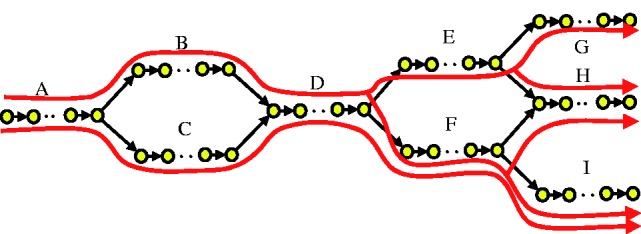
Example of de Bruijn graph for five isoforms from the same gene

(2) Different expression levels of isoforms of the same gene. Isoforms of the same gene may have very different expression levels. There are two problems. First, low-expressed isoforms may have little support from reads and thus are missed by the assembler. For example, in Figure 1, if there are only a few paired-end reads supporting branch BD and FH, isoform ABDFH is unlikely to be obtained. Second, support from reads of erroneous k-mers from high-expressed transcripts may be higher than that of correct k-mers from low-expressed transcripts. These erroneous k-mers introduce branches in the de Bruijn graph and make the graph very complicated. Figure 2 shows an example from a real rice transcriptome dataset (LOC-Os12g12850). This subgraph (k = 50) is supposed to contain only two isoforms (Fig. 2a shows the conceptual view of the isoforms). There are 92 353 and 90 126 erroneous k-mers and branches respectively in the de Bruijn graph (Fig. 2b) when we simulated reads with 1% sequencing error (details shown in Section 3). Existing approaches usually employ a global threshold to remove erroneous k-mers and branches if the multiplicities of these components are smaller than the threshold. This simple approach will not work for transcriptome data. Since the error positions of each read are known, we can count the number of correct and erroneous k-mers for simulated data on rice (Section 3.1) for different multiplicities (Fig. 2c). No matter how we set the threshold of multiplicity for removing erroneous k-mers (draw a vertical line and consider all k-mers on the left with lower multiplicities as erroneous k-mers), some erroneous k-mers will remain and correct k-mers will be removed. These complicated components will make isoform finding extremely difficult as there are many paths to be considered. In the ideal case, the de Bruijn graph should have many isolated components, each representing isoforms from one gene unless there are repeats in different genes. In most cases, the structure of the component should be simple as most genes do not contain many isoforms. To tackle this issue, we need a method to separate components that are falsely connected by erroneous k-mers and we need to remove erroneous k-mers from each component.

Fig. 2.

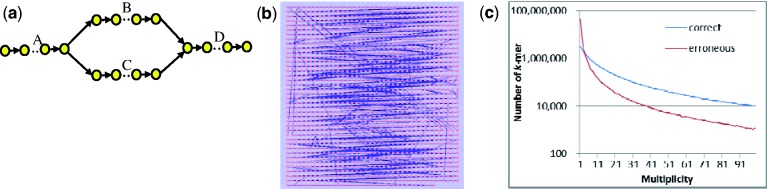
Example of de Bruijn graph for two isoforms from the same gene. (a) de Bruijn graph of two isoforms without error. (b) de Bruijn graph of two isoforms when there is 1% sequencing error in reads. (c) Multiplicity of correct and erroneous k-mers for simulated data

Existing solutions: Oases (Schulz et al., 2012) and Trinity (Grabherr et al., 2011) are two popular de novo transcriptome assemblers for RNA-Seq data. In order to solve the splicing problem [Issue (1)], both apply a dynamic programming approach to identify potential paths in the graph, which are supported by many reads or paired-end reads. In other words, they try to identify isoforms more globally through a path-level analysis instead of a local branch-level analysis. The results are much better than those of genome assemblers. However, since the problem is NP-complete (proved in the Supplementary Appendix), the running time of the dynamic programming approach increases exponentially with the number of branches in the de Bruijn graph. Due to Issue (2), erroneous reads sampled from high-expressed transcripts introduce many branches (with more support than reads sampled from low-expressed transcripts) and thus dynamic programming takes a long time. In practice, these tools fall back on heuristic search instead of dynamic programming for large components.

To tackle Issue (2), T-IDBA (Peng et al., 2011) uses another approach to isolate components. Based on the observation that transcripts from different genes share less common vertices when k value is large, T-IDBA builds a de Bruijn graph from small k and iteratively updates the graph with larger k values. It then finds transcripts in the de Bruijn graph with large k value where transcripts from the same gene usually form a single component. However, it does not perform very well for low-expressed transcripts because there are more missing k-mers when k is large. There is no dedicated solution in T-IDBA that solves the issue of erroneous k-mers within a component and methods for isolating components are not sensitive to low-expressed isoforms.

To recover low-expressed transcripts, several post-processing methods (Robertson et al., 2010; Surget-Groba and Montoya-Burgos, 2010) were developed for Velvet (Zerbino and Birney, 2008) and Abyss (Simpson et al., 2009). They are all based on the observation that lower k values make the assembler more sensitive to low-expressed transcripts, while larger k values make it more specific to high-expressed transcripts. In order to combine the advantages of different values of k, the resultant contigs, generated by different k-mer lengths independently, are merged together.

However, merging assembly results from different runs is not a straightforward task. Although output transcripts are clustered and duplicated transcripts are removed, many duplicates are difficult to detect and errors can accumulate in the cluster-remove step. As a result, multiple contigs with errors are generated for the same transcripts and the number of resulting contigs is much more than the number of expressed transcripts. Oases-M, an extension of Oases, makes use of multiple k to improve its assembly result and is now the best tool using this approach. However, since the fundamental problem of removing erroneous vertices from high-expressed isoforms while keeping correct vertices from low-expressed isoforms is not solved, there are still many false positives as well as duplicated transcripts (Section 3).

Some single-cell genome assemblers (Chitsaz et al., 2011; Peng et al., 2012) also have a problem with uneven multiplicities of correct k-mers. They resolve the problem based on the assumption that, although the multiplicities of these erroneous k-mers are high, their multiplicities should be lower than the nearby correct k-mers. Thus, they calculate a local threshold, based on the multiplicities of nearby k-mers or contigs, for removing erroneous k-mers. However, as a k-mer representing the common exon of several expressed isoforms can have relatively higher multiplicity than nearby correct k-mers (Li and Jiang, 2012), calculating the local threshold from only one or two nearby k-mers or contigs may be misleading and the algorithms may remove many correct k-mers near these high multiplicity k-mers.

Our contributions: If Issue (2) can be resolved, Issue (1) can be tackled by existing path-level analysis as the components will be simple enough. Thus, our core contribution is handling Issue (2). As mentioned before, the traditional filtering method of using one single global threshold for multiplicity cannot separate correct k-mers sampled from low-expressed transcripts from erroneous k-mers sampled from high-expressed transcripts, and single-cell genome assemblers calculating local thresholds from nearby k-mers may remove many correct k-mers. Thus, we propose a probabilistic progressive approach to solve this problem. Our proposed assembler IDBA-Tran calculates the probability that a k-mer or short simple path (contigs) contains error using not only the multiplicity of the k-mer or contig (or their neighboring k-mers or contigs) but also uses a multi-normal distribution to model the multiplicities of all k-mers in the whole connected component. Based on the multi-normal distribution and the contig length (as a short simple path is more likely to have error than a long one), IDBA-Tran calculates a local threshold for determining whether a k-mer or contig has error. By progressively removing erroneous k-mers, connected components representing isoforms from a single gene are identified. Since we successfully remove many erroneous k-mers, the size of each component is small. We can employ a path-level analysis (similar to Oases and Trinity) to identify transcripts from each component [Issue (1)]. Thus IDBA-Tran can perform better than Oases and Trinity, producing more contigs, particularly for low-expressed transcripts. Results show that IDBA-Tran outperforms other de novo transcriptome assembly approaches in terms of both sensitivity and specificity for both simulated and real data. IDBA-Tran also makes use of other techniques used in genome assemblers, such as tips pruning, path merging and error correction.

2 METHODS

Similar to Oases-M, IDBA-Tran also adopts the idea of multiple k to handle transcripts with different expression levels. However, instead of generating a de Bruijn graph and finding transcripts for each k value, an accumulated de Bruijn graph is built to capture all information from both high-expressed and low-expressed transcripts. During each iteration, an accumulated de Bruijn graph H_k for a fixed k is constructed from the input reads and the contigs constructed in previous iterations, i.e. those contigs constructed in H_k-s are treated as input reads for the construction of H_k. The depth information is used to separate de Bruijn graph into components. Ideally, transcripts from different genes are decomposed into different components. In each component, alternative splicing can be detected and transcripts can be reconstructed. To accumulate information, all reconstructed transcripts are used as input reads for the next iteration.

Figure 3 shows the workflow of IDBA-Tran for assembling a set of paired-end reads. In the first iteration when k = k_min, H_k is equivalent to a de Bruijn graph for vertices whose corresponding k-mers have multiplicity of at least m (2 by default) times in all reads. During all subsequent iterations, sequencing errors are first removed according to the topological structure of H_k in a slightly different way to other assemblers (Section 2.1). The tips (dangling paths in H_k of length shorter than 2k) are likely to be false positives (Li et al., 2010; Simpson et al., 2009; Zerbino and Birney, 2008). Similar paths (bubbles) representing very similar contigs with the same starting vertex and ending vertex are likely to be caused by errors or SNPs and they should be merged (Li et al., 2010; Simpson et al., 2009; Zerbino and Birney, 2008). Then, the depth information for contigs and components is used to decompose the graph into components (Section 2.2). Paths with high support for the paired-end reads are reconstructed as transcripts in each component (Section 2.3). Errors in the assembled contigs are corrected by aligning reads to the contigs (Section 2.4). When constructing H_k+s from H_k, each length s + 1 path in H_k is converted into a vertex ((k + s)-mer) and there is an edge between two vertices if the corresponding (k + s + 1)-mer appears f (1 by default) times in reads or once in contigs in C_k∪LC_k∪T_k, where C_k represents the set of contigs, LC_k is the set of contigs constructed by local assembly using paired-end information (Section 2.5), and T_k is the set of transcripts when considering H_k. In the following subsections, we describe each step of IDBA-Tran in detail.

Fig. 3.

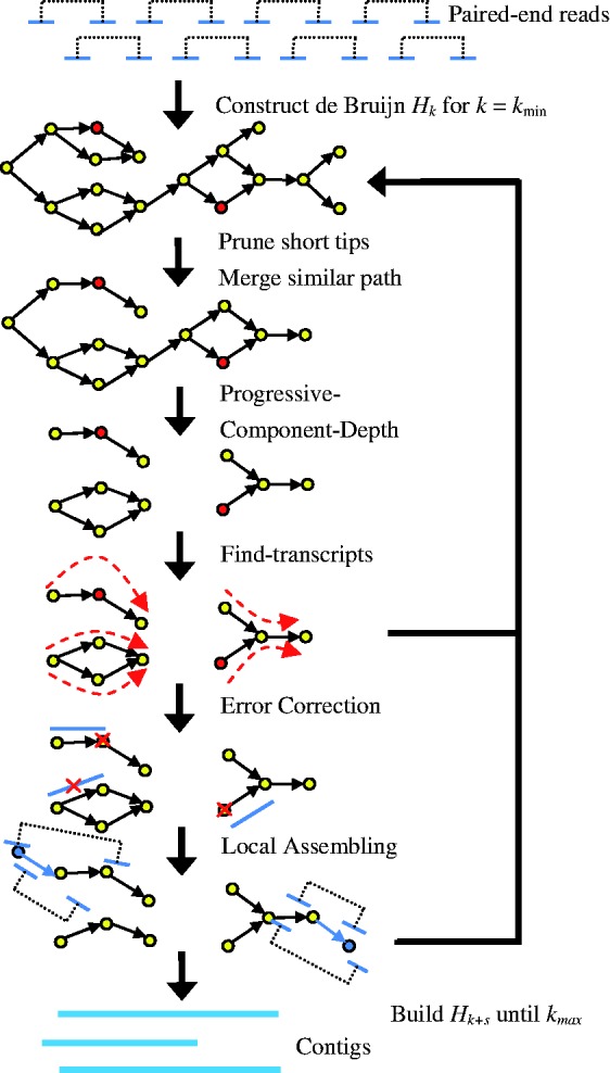
Workflow of IDBA-Tran

2.1 Pruning short tips and merge similar path

Many de novo assemblers remove tips (short simple paths leading to dead ends) in the de Bruijn graph as erroneous contigs. It would not be advisable to remove such tips in transcriptome assembly, because transcripts are very short (could be several hundred bases) when compared to genomes. Removing one hundred bases from the end of a genome may not be a problem, but removing one hundred bases from the end of a transcript may lose much important information. When constructing the accumulated de Bruijn graph in IDBA-Tran, the tip removal process will take place at each iteration. Instead of removing all tips and producing shorter transcripts, IDBA-Tran keeps the longest tip (with highest probability of being a correct path) and removes all other short tips. For each branch in the graph, IDBA-Tran checks each outgoing (and incoming) edge, keeps the branch which leads to the longest path, and removes all other branches (tips) which lead to paths shorter than 2k. Usually, the correct branch leads to longer paths than tips, and this method preserves correct branches.

As transcriptome sequencing data contains more errors and insertions/deletions than genome sequencing data, IDBA-Tran identifies and merges paths with same starting point and end point and higher than 98% similarity (including insertions and deletions).

2.2 Decomposing the graph by iterating depth

Recall that T-IDBA (Peng et al., 2011) also tries to decompose the de Bruijn graph into components. It is based on the observation that there are not many repeat patterns between two transcripts from different genes while isoforms from the same gene share common exons. Thus, it decomposes the graph into different components such that there are relatively more branches inside each component and relatively fewer branches between two components. However, erroneous k-mers (from high-expressed isoforms) still cannot be removed effectively since components representing isoforms from different genes may be connected by these erroneous k-mers to form a very large component preventing the assembler from determining isoforms in the component. Instead of considering the number of branches for decomposing the de Bruijn graph into components, IDBA-Tran detects and removes erroneous paths connecting two components by considering the lengths and sequencing depths (depths in short) of the paths using a probabilistic approach. The depth of a path (contig) is the average multiplicity of the k-mer on the path.

Long contigs (simple paths in the de Bruijn graph) are usually correct, because long simple paths are unlikely to be formed by erroneous reads, and similarly for high-depth contigs which have supports from many reads. For a contig, whether its length is long or short and whether its depth is high or low cannot be judged by absolute values as the length of a contig depends on the value of k and the depth of a contig depends on the depths of neighboring contigs (contigs in the same component). Since erroneous contigs in high-depth regions may have higher depths than correct contigs in low-depth regions, short (<l) and relatively low-depth contigs are likely to be erroneous and can be removed. The removal takes place in an iterative manner (Chitsaz et al., 2011; Peng et al., 2012), because after some low-depth errors are removed, some short low-depth contigs may be connected together to form long contigs. Increasing depth cutoff progressively may help to preserve more low-depth correct contigs.

IDBA-Tran removes contigs (simple paths) shorter than l with average sequencing depth lower than β where β is a threshold calculated based on value of l and the depth distribution of the connected component which contains the contig. When β is large, many correct contigs are removed and many true positive transcripts cannot be assembled. When β is small, many erroneous contigs are not removed and transcripts from different genes may form a large component such that correct transcripts are difficult to reconstruct in later steps (Section 2.3). Thus, we should select the largest threshold β such that not too many correct contigs are removed, say <1%.

Consider a correct exon with length at least l. It should be represented by a simple path P in the de Bruijn graph. However, as there are sequencing errors in reads, there may be branches in P and simple path P may be broken into several shorter paths with length less than l. Consider a particular edge u→v in P with the corresponding k-mer v sampled x times (some may contain errors). There is another edge u→v’ in the de Bruijn graph if at least m (the multiplicity threshold used for removing erroneous k-mers) out of the x k-mers sampled from v having the same error at the last nucleotide, i.e. v and v’ differ by the last nucleotide, thus introduces branching at u. This probability can be calculated as follows.

Assume the probability of a sequencing error per base is e and the probabilities that the erroneous base is changed to each other nucleotide are the same, i.e. 1/3. Although this simple assumption is not correct for real biological data, the calculation can be readily refined for different probabilities. The probability that v is sampled as v’ with the last nucleotide changed to a particular nucleotide, say ‘A’, is

As v can be sampled with error as v’, i.e. at least m of the x samples have the same error at the last nucleotide. Since there are three possible v’, the existence probability of v’ (probability of branching at u) is

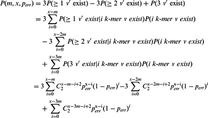In order to estimate the value of depth x, we use a multi-normal distribution to model the depth distribution of a component as there can be multiple isoforms, say t, in a component. Given a set of k-mers with different multiplicities in the same component, we assume the multiplicities of the k-mers are sampled from t normal distributions. Although the mean and standard deviation of each normal distribution can be estimated by expectation-maximization algorithm (Tanaseichuk et al., 2012), the time is too long because there are many k-mers and components. Thus IDBA-Tran applies an approximation by clustering the k-mers based on their multiplicities (the distance between two k-mers equals their difference in multiplicities) using K-means clustering method. The mean and standard deviation can then be calculated for each cluster. We set t = 3 in the experiments based on the assumption that there are at most 3 transcripts in each components (at the final step).

Let N(μ, σ) be a normal distribution of depth with minimum mean depth value μ. The probability that we wrongly remove a correct contig with average depth ≤ β is at most

Note that for an exon of length at least l of sequencing depth x, the probability of branching is .

The value of l should be selected based on the length of exons. If a very large l is selected, true positive k-mers and paths are removed. If a very small l is selected, most true negative k-mers and paths cannot be removed. We should select different values for l depending on the properties of the data (we use l = 2k in the experiments). Once l is selected, we can calculate the largest β such that P(false positive) is lower than some value, say 1%, so as to remove most erroneous contigs without too many false positives.

Algorithm 1 shows the pseudocode for the decomposing step. According to (Peng et al., 2011), when the size of the component is small (with ≤ γ = 30 contigs), the component is likely to represent isoforms from a single gene and we can use a very low depth threshold β = 0.1 × T(comp), where T(comp) is the average depth of connected component comp, to prevent removing correct contigs. The filtering depth cutoff threshold t is increased by a factor of α progressively (10% by default). In each iteration, short contig c is removed if its depth T(c) is lower than the minimum of cutoff threshold t and the depth threshold β.

2.3 Finding transcripts

Algorithm 1. Progressive-Component-Depth(G, k).

 t ← 1

 repeat until t > max_c∈GT(c)

  for each component comp in G

   if size(comp) > γ, then calculate β, else β ← 0.1 × T(comp)

   for each contig c in comp

 if len(c) < 2k and T(c) < min(t, β)

 remove c from G

 t ← t × (1 + α)

For each connected component in the de Bruijn graph, IDBA-Tran discovers those paths starting from a vertex with zero in-degree to a vertex with zero out-degree with the highest support from paired-end reads. A path is supported by paired-end reads if the paired-end reads can be aligned to the path with the distance between the aligned positions matching the insert distance of the paired-end reads. The problem definition can be simplified as follows [Transcripts Discovering (TD) Problem]: given a de Bruijn graph G(V, E) with a set of vertices V and edges E, a set of paired-end reads P = {(v_i, v_j)}, v_i, v_j ∈ V, an insert distance d and error s, find t paths in G with the maximum number of supporting paired-end reads P’ ⊆ P. A path p has a supporting paired-end read (v_i, v_j) iff p contains vertices v_i and v_j and the distance between v_i and v_j in p is between d – s and d + s.

Since the TD problem is a NP-hard problem (see Supplementary Appendix), IDBA-Tran performs a heuristic depth-first search to find paths from a zero in-degree vertex to a zero out-degree vertex with maximum supporting paired-end reads. At each branch, the path with many supporting paired-end reads will be considered before other paths. In practice, IDBA-Tran reports at most t_max (default 3) potential transcripts for each zero in-degree vertex in each connected component. IDBA-Tran applies a seed and extend method for aligning reads to contigs (paths in de Bruijn graph). k-mers in a read appearing in the de Bruijn graph is considering as potential aligned position and IDBA-Tran will try to extend both ends of alignment considering substitution error only. Note that insertion and deletion error can be implemented in IDBA-Tran easily. However, as the number of substitution errors appears much more than the insertion/deletion errors, IDBA-Tran considers substitution error only for speeding up the alignment process.

2.4 Error correction

The error correction step is performed on reads and assembled contigs during the assembling process. At first, reads are aligned to each contig. The consensus of the aligned reads will replace the original contig, i.e. positions of the contig inconsistent with the majority of aligned reads will be corrected. Then aligned reads are corrected according to the aligned position in contigs, i.e. positions in the reads with nucleotides inconsistent with the consensus will be corrected. This error correction step can reduce the number of erroneous reads and branches in the de Bruijn graph.

2.5 Local assembly

Let C be the set of contigs. We extract the beginning and end of each contig c in C to form a set of contigs C'. Assume the insert distances of paired-end reads satisfy the normal distribution N(d, δ). IDBA-Tran performs local assembly (Peng et al., 2012) on the last d + 3δ bases of each end of the contig and the paired-end read with one end aligned to it. Since those reads which are far away from contig c will not mix with reads with one end aligned to c, some missing k-mers can be reconstructed and the contigs can be extended longer.

2.6 Estimating expression levels

Since IDBA-Tran is designed for assembling reads to reconstruct expressed transcripts, sophisticated algorithms can be then applied to estimate the expression levels of each transcript. IDBA-Tran also provides an estimated expression level for each transcript by aligning reads to the transcript. RPKM (Reads Per Kilobase per Million mapped reads) is estimated by dividing the total length of reads uniquely aligned to a transcript by the total length of regions of transcript uniquely aligned by reads.

3 RESULTS

To evaluate the performance of IDBA-Tran, experiments were carried out on both simulated and real data. We compared IDBA-Tran with the latest transcriptome assemblers Trinity (Grabherr et al., 2011) and Oases (Schulz et al., 2012). We also compared IDBA-Tran with the single-cell genome assembler IDBA-UD (Peng et al., 2012) and Velvet-SC (Chitsaz et al., 2011), which apply multiple depths when assembling genomes. IDBA-Tran and IDBA-UD were run with k ranging from 20 to 50 with step size 5. For Oases and Velvet-SC, k values ranging from 20 to 50 with step size 5 were used, and the best result was selected as output. As the k value of Trinity was fixed to 25, the default parameters were used to run it.

For transcriptome assembly, the most important indicator of assembly quality is the number of correct transcripts an assembler can reconstruct. In the experiments, known transcript references were used for benchmarking. A known transcript is reconstructed successfully if a certain portion, say 80% (referred as completeness), of its sequence is covered by a contig with 95% similarity. Similarly, the contig is considered correct if it can be aligned to at least 80% of a transcript with 95% similarity. The alignment of contigs to transcripts was performed by BLAT (Kent, 2002) without considering long gaps representing introns (as we aligned contigs to transcripts instead of genome). The sensitivity and specificity were calculated to measure performance. Sensitivity is the percentage of reconstructed transcripts over all expressed transcripts. Specificity is the percentage of correct contigs over all reported contigs.

We also compared the performance of IDBA-Tran and CEM (Li and Jiang, 2012) on estimating expression levels of reconstructed transcripts. CEM requires the genome sequence as additional information. By aligning reads to the reference genome, CEM can predict the expressed transcript sequences and estimate the expression level of each transcript based on a statistical model (quasi-multinomial model). Since some transcripts may align to multiple contigs and some contigs may align to multiple transcripts, we considered only those transcripts and contigs with one-to-one correspondence. The Pearson’s correlation between the predicted expression levels and the exact expression levels was calculated. As suggested in Li and Jiang, 2012, we also calculated the Pearson’s correlation between the logarithm of predicted expression levels and the logarithm of exact expression levels.

3.1 Simulated data

In order to simulate more realistic data, we aligned all reads in a real RNA-Seq data of Oryza sativa Transcriptome to known transcripts of Oryza sativa in the database. Based on the alignment results, we identified the set of expressed transcripts and estimated their expression levels. Note that, since the transcript sequences were known, no long gap (representing an intron) alignments were allowed. Reads aligned to multiple transcripts were not considered for estimating the depth of the transcript. We used all transcripts with at least 80% of the region aligned by reads and with depth at least 0.5× to generate the simulated data, i.e. there were 0.5 reads covering each nucleotide on average. We sampled paired-end reads from the transcripts according to their expression levels. The read length was 100 bp, error rate was 1% and the insert distance followed a normal distribution with mean 250 bp and standard deviation 25 bp.

Figure 4 shows the quality of the assembly results of the assemblers for different levels of completeness. Velvet-SC reconstructed the least number of transcripts in all completeness settings because it is designed for assembling genomic data and cannot handle multiple isoforms of the same gene well. IDBA-UD, which is designed for assembling genomic and metagenomic data, handled some simple cases of multiple isoforms of the same gene and had better performance than Velvet-SC. Trinity and Oases found more transcripts than Velvet-SC and IDBA-UD because they are designed for assembling transcriptome data. Oases had its best performance when k was set to 25, the same k value for Trinity. IDBA-Tran reconstructed the most transcripts and consistently reported more correct contigs. Table 1 shows the detailed figures when completeness was 0.8. The number of correct contigs and reconstructed transcripts for IDBA-Tran were the highest among the tools. IDBA-Tran also had the highest sensitivity and specificity.

Fig. 4.

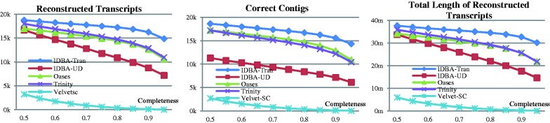
Experiment result of each assembler on different completeness level for simulated data

Table 1.

Statistics of assembly result of each assembler for simulated data set (completeness = 0.8)

	Contigs number	Average length (nt)	Total length (nt)	Reconstructed transcripts number	Correct contigs number	Sensitivity	Specificity
Trinity	26 189	1941	41M	14 910	14 389	66.56%	54.94%
Oases	22 804	1963	39M	14 420	14 712	64.37%	64.51%
IDBA-UD	18 020	1322	24M	10 941	8406	48.58%	46.65%
Velvet-SC	22 868	613	14M	389	357	1.74%	1.56%
IDBA-Tran	22 708	1933	39M	17 242	16 707	76.98%	73.57%

Table 2 shows the expression level distribution of reconstructed transcripts of the assemblers when completeness was 0.8. For low-expressed transcripts with sequencing depth <5, IDBA-Tran reconstructed 664 more transcripts (33% more) than the second best tool (Trinity). This is probably due to the fact that IDBA-Tran can separate transcripts from different genes into components efficiently while preserving the low-expressed transcripts. We also checked the quality of decomposition and found that over 80% of the transcripts were still inside the same component after the decomposition step (referred to “unbroken transcripts after decomposition). Except transcripts with very low sequencing depth (<5), most transcripts were not broken after the decomposition and could be constructed successfully. Similar results were found for transcripts with sequencing depth between 5 and 10. For transcripts with higher sequencing depth, in general, IDBA-Tran also performed better (even though all assemblers had better performance for high-expressed transcripts).

Table 2.

Expression level distribution of reconstructed transcripts of each assembler for simulated data set (completeness = 0.8)

Depth	0, 5	5, 10	10, 15	15, 20	≧20
Total number of transcripts	5943	5011	2943	1857	6646
Trinity	1955	3251	2393	1527	5782
Oases	1648	3224	2461	1606	5481
IDBA-UD	1629	2563	1753	1107	3831
Velvet-SC	58	139	106	55	31
IDBA-Tran (unbroken transcripts after decomposition)	2619 (2700)	4177 (4337)	2746 (2824)	1723 (1811)	5977 (6505)

For IDBA-Tran, we verified the effectiveness of its component separation algorithm and show the distribution of transcripts in Table 3. If a component contained a certain portion (80%) of a transcript, the component was deemed to have contained this transcript. There were 2865 components containing no transcripts and 10 611 components, each of which contained at most 5 transcripts, together containing most of the transcripts (16 663). Since very low-expressed transcripts cannot be assembled by any assemblers, the total number of transcripts (18 180) in all components was less than the total number of expressed transcripts (22 402). A component containing a transcript does not guarantee that the transcript can be reconstructed. Thus, the number of reconstructed transcripts (17 243) is less than the total number of transcripts in all components (18 180). However, experiments showed that most transcripts decomposed correctly can be reconstructed successfully.

Table 3.

Distribution of transcripts in IDBA-Tran components for simulated data set (completeness = 0.8)

Transcripts in component	0	1	2	3	4	5	6	7	8	9	≥10	Total
Number of components	2865	6722	2407	954	370	158	71	28	24	4	22	13 625
Number of unbroken transcripts (after decomposition)	0	6720	4814	2859	1480	790	426	196	192	37	666	18 180
Number of reconstructed transcripts	0	6676	4682	2672	1324	667	349	164	141	33	535	17 243

Table 4 shows the performance of IDBA-Tran and CEM on estimating expression levels of transcripts. Although CEM had the additional information of the rice genome, the number of expression transcripts reconstructed by IDBA-Tran and CEM were similar. Moreover, IDBA-Tran had similar performance to CEM in estimating the expression levels because it could reconstruct most of the expressed transcripts making the estimation process easier.

Table 4.

Statistic on estimating expression levels of reconstructed transcripts of each assembler for simulated data set (completeness = 0.8)

	Transcripts reconstructed by both algorithms		Transcripts reconstructed by only one algorithm
	Number of transcripts	Pearson’s correlation (based on log value)	Number of transcripts	Pearson’s correlation (based on log value)
CEM	5611	0.95 (0.91)	100	0.89 (0.79)
IDBA-Tran		0.95 (0.94)	37	0.93 (0.85)

3.2 Real data

We verified IDBA-Tran and other assemblers on the real RNA-Seq data of Oryza sativa transcriptome. There were 24 855 142 paired-end length-90 reads in the data set. The insert distance was about 200. Previous simulated data used the expression level profile of this data set, so they had the same set of expressed transcripts and expression levels. The distribution of expressed transcripts is also included in Table 6 for comparison (with the distribution of expressed transcripts estimated as mentioned in Section 3.1). Note that since the expressed transcripts and expression levels were estimated from alignments, there may be some error due to the existence of unknown transcripts and transcripts with over 80% similarity. The sensitivities and specificities shown are approximation of the real sensitivities and specificities only.

Table 6.

Expression level distribution of reconstructed transcripts of each assembler for real data set (completeness = 0.8)

Depth	0, 5	5, 10	10, 15	15, 20	≧20
Total number of transcripts	5943	5011	2943	1857	6646
Trinity	410	910	983	743	4004
Oases	431	907	1005	776	3946
IDBA-UD	287	978	985	723	3124
Velvet-SC	28	55	55	28	67
IDBA-Tran (unbroken transcripts after decomposition)	732 (921)	1480 (1525)	1417 (1472)	1041 (1083)	4758 (5325)

Figure 5 shows the number of reconstructed transcripts and aligned (correct) contigs reported by each assembler under different completeness. The results were consistent with those for the simulated data. IDBA-Tran still performed the best for all levels of completeness. All assemblers had poorer performance for real data than for simulated data. Oases still had its best performance when k was set to 25, and had very similar performance in terms of reconstructed transcripts compared with Trinity in all completeness settings.

Fig. 5.

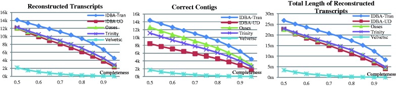
Experiment result of each assembler on different completeness level for real data

Detailed statistics of assembly results are shown in Table 5 when completeness is set to 0.8. IDBA-Tran, Oases and Trinity had about the same number of contigs and total contig bases. IDBA-UD assembled relatively fewer contigs than others. IDBA-Tran had the highest sensitivity (42.08%) and specificity (22.94%) while other assemblers had much lower sensitivity and specificity.

Table 5.

Statistics of assembly result of each assembler for real data set (completeness = 0.8)

	Contigs number	Average length (nt)	Total length (nt)	Reconstructed transcripts number	Correct contigs number	Sensitivity	Specificity
Trinity	39 974	966	39M	7052	6121	31.48%	15.31%
Oases	36 684	1041	38M	5666	5162	25.29%	14.07%
IDBA-UD	28 753	890	25M	6164	4567	27.51%	15.88%
Velvet-SC	28 626	518	15M	233	208	1.04%	0.73%
IDBA-Tran	40 010	1055	42M	9428	9177	42.08%	22.94%

Table 6 shows the expression level distribution of reconstructed transcripts for different assemblers when completeness is set to 0.8. When comparing Tables 2 and 6, it is clear that the real data was more difficult to assemble than simulated data, especially for low-expressed transcripts. Only 732 transcripts (∼25%) with depth <5 were reconstructed by IDBA-Tran and worse for other assemblers. Similar to simulated data, IDBA-Tran had better performance than other assemblers for all expression levels.

Table 7 shows the distribution of transcripts in components. Since the sampling depths of a single transcript may be uneven, many transcripts were broken into fragments. Moreover, there were some unknown transcripts in the data set. So, quite a number of components did not contain 80% of a transcript. However, for the other components, IDBA-Tran did a good job: 6353 components, each of which contained at most 5 transcripts, contained 9082 transcripts all together. Similar to simulated data, once a transcript was correctly assigned to a component, the transcript was reconstructed with high probability.

Table 7.

Distribution of transcripts in IDBA-Tran components for real data set (completeness = 0.8)

Transcripts in component	0	1	2	3	4	5	6	7	8	9	>=10	total
Number of components	20 288	4482	1265	408	145	53	21	17	6	6	15	26 706
Number of unbroken transcripts (after decomposition)	0	4482	2531	1224	580	265	126	119	48	54	593	10 022
Number of reconstructed transcripts	0	4371	2450	1152	553	265	126	119	48	28	316	9428

4 DISCUSSION

We have identified one key issue in transcriptome assembly, namely how to remove erroneous vertices/edges of high multiplicity (due to high-expressed isoforms) from the de Bruijn graph while keeping correct ones with relatively lower multiplicity (due to low-expressed isoforms). We developed a probabilistic progressive approach with local thresholds to solve the problem. We proposed IDBA-Tran, combined with other techniques, to assemble transcriptome sequencing data. Experiments on both simulated and real data confirm that IDBA-Tran can outperform existing de novo transcriptome assemblers in terms of both sensitivity and specificity. In particular, for low-expressed transcripts, the improvement of IDBA-Tran is substantial.

Recall that there is another approach to recover both low-expressed and high-expressed transcripts, namely: run the assembler for different k values and merge all contigs as output. Oases-M, which runs Oases several times with multiple k values, is a post-processing tool based on this approach. Oases-M can reconstruct many transcripts for both simulated and real data. However, since erroneous contigs cannot be merged, Oases-M produces many incorrect contigs and has a low specificity (see Supplementary Table SA8). Moreover, contigs representing some transcripts may appear multiple times (with small difference) in the output such that the number of correct contigs is double the number of reconstructed transcripts. The large number of erroneous contigs and redundant contigs may make analysis difficult, and it is very hard to distinguish the erroneous contigs from the correct ones. On the other hand, we found that Oases-M had slightly better performance than IDBA-Tran for high-expressed transcripts for real data (see Supplementary Table SA9). Thus, it may be a good idea to investigate how to integrate both approaches to reconstruct more transcripts.

Funding: This research is partially supported by RGC HKU 7111/12E and HKU 719709E, the Shanghai Pujiang Plan (Y057C11501) and Bill & Melinda Gates Foundation Project (“C4 Rice”).

Conflict of Interest: none declared.

REFERENCES

- Bankevich A, et al. SPAdes: a new genome assembly algorithm and its applications to single-cell sequencing. J. Comput. Biol. 2012;19:455–477. doi: 10.1089/cmb.2012.0021. [DOI] [PMC free article] [PubMed] [Google Scholar]
- Chitsaz H, et al. Efficient de novo assembly of single-cell bacterial genomes from short-read data sets. Nat. Biotechnol. 2011;29:915–921. doi: 10.1038/nbt.1966. [DOI] [PMC free article] [PubMed] [Google Scholar]
- Grabherr MG, et al. Full-length transcriptome assembly from RNA-Seq data without a reference genome. Nat. Biotechnol. 2011;29:644–652. doi: 10.1038/nbt.1883. [DOI] [PMC free article] [PubMed] [Google Scholar]
- Graveley BR. Molecular biology: power sequencing. Nature. 2008;453:1197–1198. doi: 10.1038/4531197b. [DOI] [PMC free article] [PubMed] [Google Scholar]
- Guttman M, et al. Ab initio reconstruction of cell type-specific transcriptomes in mouse reveals the conserved multi-exonic structure of lincRNAs. Nat. Biotechnol. 2010;28:503–510. doi: 10.1038/nbt.1633. [DOI] [PMC free article] [PubMed] [Google Scholar]
- Li W, Jiang T. Transcriptome assembly and isoform expression level estimation from biased RNA-Seq reads. Bioinformatics. 2012;28:2914–2921. doi: 10.1093/bioinformatics/bts559. [DOI] [PMC free article] [PubMed] [Google Scholar]
- Jiang H, Wong WH. Statistical inferences for isoform expression in RNA-Seq. Bioinformatics. 2009;25:1026–1032. doi: 10.1093/bioinformatics/btp113. [DOI] [PMC free article] [PubMed] [Google Scholar]
- Kent WJ. BLAT–the BLAST-like alignment tool. Genome Res. 2002;12:656–664. doi: 10.1101/gr.229202. [DOI] [PMC free article] [PubMed] [Google Scholar]
- Li R, et al. The sequence and de novo assembly of the giant panda genome. Nature. 2010;463:311–317. doi: 10.1038/nature08696. [DOI] [PMC free article] [PubMed] [Google Scholar]
- Nagalakshmi U, et al. The transcriptional landscape of the yeast genome defined by RNA sequencing. Science. 2008;320:1344–1349. doi: 10.1126/science.1158441. [DOI] [PMC free article] [PubMed] [Google Scholar]
- Peng Y, et al. RECOMB. Vancouver, BC, Canada: 2011. T-IDBA: a de novo Iterative de Bruijn Graph Assembler for Transcriptome. [Google Scholar]
- Peng Y, et al. IDBA-UD: a de novo assembler for single-cell and metagenomic sequencing data with high uneven depth. Bioinformatics. 2012;28:1420–1428. doi: 10.1093/bioinformatics/bts174. [DOI] [PubMed] [Google Scholar]
- Robertson G, et al. De novo assembly and analysis of RNA-seq data. Nat/ Methods. 2010;7:909–912. doi: 10.1038/nmeth.1517. [DOI] [PubMed] [Google Scholar]
- Schulz MH, et al. Oases: robust de novo RNA-seq assembly across the dynamic range of expression levels. Bioinformatics. 2012;28:1086–1092. doi: 10.1093/bioinformatics/bts094. [DOI] [PMC free article] [PubMed] [Google Scholar]
- Simpson JT, et al. ABySS: a parallel assembler for short read sequence data. Genome Res. 2009;19:1117–1123. doi: 10.1101/gr.089532.108. [DOI] [PMC free article] [PubMed] [Google Scholar]
- Surget-Groba Y, Montoya-Burgos JI. Optimization of de novo transcriptome assembly from next-generation sequencing data. Genome Res. 2010;20:1432–1440. doi: 10.1101/gr.103846.109. [DOI] [PMC free article] [PubMed] [Google Scholar]
- Tanaseichuk O, et al. A probabilistic approach to accurate abundance-based binning of metagenomic reads. Algorithms Bioinform. 2012;7534:404–416. [Google Scholar]
- Trapnell C, et al. TopHat: discovering splice junctions with RNA-Seq. Bioinformatics. 2009;25:1105–1111. doi: 10.1093/bioinformatics/btp120. [DOI] [PMC free article] [PubMed] [Google Scholar]
- Trapnell C, et al. Transcript assembly and quantification by RNA-Seq reveals unannotated transcripts and isoform switching during cell differentiation. Nat. Biotechnol. 2010;28:511–515. doi: 10.1038/nbt.1621. [DOI] [PMC free article] [PubMed] [Google Scholar]
- Vyahhi N, et al. From de Bruijn Graphs to Rectangle Graphs for Genome Assembly. LNCS. 2012;7534:249–261. [Google Scholar]
- Zerbino DR, Birney E. Velvet: algorithms for de novo short read assembly using de Bruijn graphs. Genome Res. 2008;18:821–829. doi: 10.1101/gr.074492.107. [DOI] [PMC free article] [PubMed] [Google Scholar]
Associated Data
This section collects any data citations, data availability statements, or supplementary materials included in this article.