Statistical Measures on Residue-Level Protein Structural Properties

Abstract

Background

The atomic-level structural properties of proteins, such as bond lengths, bond angles, and torsion angles, have been well studied and understood based on either chemistry knowledge or statistical analysis. Similar properties on the residue-level, such as the distances between two residues and the angles formed by short sequences of residues, can be equally important for structural analysis and modeling, but these have not been examined and documented on a similar scale. While these properties are difficult to measure experimentally, they can be statistically estimated in meaningful ways based on their distributions in known proteins structures.

Results

Residue-level structural properties including various types of residue distances and angles are estimated statistically. A software package is built to provide direct access to the statistical data for the properties including some important correlations not previously investigated. The distributions of residue distances and angles may vary with varying sequences, but in most cases, are concentrated in some high probability ranges, corresponding to their frequent occurrences in either α-helices or β-sheets. Strong correlations among neighboring residue angles, similar to those between neighboring torsion angles at the atomic-level, are revealed based on their statistical measures. Residue-level statistical potentials can be defined using the statistical distributions and correlations of the residue distances and angles. Ramachandran-like plots for strongly correlated residue angles are plotted and analyzed. Their applications to structural evaluation and refinement are demonstrated.

Conclusions

With the increase in both number and quality of known protein structures, many structural properties can be derived from sets of protein structures by statistical analyses and data mining, and these can even be used as a supplement to the experimental data for structure determinations. Indeed, the statistical measures on various types of residue distances and angles provide more systematic and quantitative assessments on these properties, which can otherwise be estimated only individually and qualitatively. Their distributions and correlations in known protein structures show their importance for providing insights into how proteins may fold naturally to various residue-level structures.

Background

The detailed atomic-level structural properties of proteins, such as bond lengths, bond angles, and torsion angles, have been well studied and understood based on either chemistry knowledge or a statistical analysis of sets of structures [1,2]. For example, we have learned that the bond lengths and bond angles are relatively fixed for most types of bonds, and the torsion angles rather than being continuously populated have distinct preferences. The knowledge of these properties has been crucial for both theoretical and experimental approaches to protein modeling. Potential functions have been defined for bond lengths, bond angles, and torsion angles using their known or preferred values [3]. Energetically favourable structures can be obtained when these potentials along with other non-bond potentials are combined and minimized [4]. In either NMR or X-ray crystallography, these properties have been used to refine an initial experimental model, which may otherwise have little atomic detail. In particular, in NMR, the experimental NOE data is mainly for hydrogen-hydrogen interactions, which is insufficient for fully determining a structure without utilizing other data on bond lengths and bond angles [5]. The correlations among these properties have been an important source of information as well. For example, a statistical analysis showed that the ϕ-ψ torsion angles around the two bonds connecting to the C_α atom in the backbones of the residues have a special correlation: When the ϕ angle is chosen for some value, the ψ angle has only a restricted range of choice, and vice versa. The information about this correlation has been employed in both experimental determination and theoretical prediction of protein structures [6,7]. The statistical distribution of the ϕ-ψ angles in known proteins has been depicted in a two-dimensional graph called the Ramachandran Plot (Fig. 1) named after the biophysicist G. N. Ramachandran who first did such a statistical survey of structures [8]. The Ramachandran Plot has been widely used for structure evaluation. By evaluating the ϕ-ψ angles for all residues in a given protein structure and putting them onto the Ramachandran Plot, one can tell whether or not the structure is well formed based on how many of the ϕ-ψ angle pairs are in the usually dense regions of the Plot. Structural properties similar to those described above can also be found at the residue-level such as the distances between two neighboring residues; the angles formed by three residues in sequence; and the torsion angles of four residues in sequence. Proteins are often modelled in a reduced form, with residues considered as basic units. The residue distances and angles then become crucial for the description of the model, and they can be as important as those at the atomic-level for structural determination, prediction, and evaluation. The knowledge on these distances and angles can also be used to define residue-level potential functions so that potential energy minimization and dynamics simulation can be performed more effectively and efficiently at the residue instead of atomic-level, because the number of variables is substantially reduced and the time step may be increased [9,10]. However, the residue distances and angles have not been examined and documented in similar detail as those at the atomic-level. The reason is that they are not easy to measure directly; the physics for the interactions between residues is not as clear; and they are not as rigid as the bond lengths and bond angles, i.e., their values are likely to vary over a wide range. While residue distances and angles are difficult to measure experimentally, they can nonetheless be estimated statistically, based on their distributions in sets of known protein structures. Such approaches have been used for extracting residue contact statistics starting in early 1980s [11]; for developing residue-level distance-based mean-force potentials [12]; for refining X-ray crystallography determined structures [13,14]; and for deriving distance and angle constraints and potentials for NMR structure refinement [15–18]. Several online databases have also been built for direct access to the statistical data on various types of distances or angles [19,20]. In the present work, we download a large number of high-resolution X-ray structures from PDB Data Bank [21], and collect and analyze several important residue-level structural properties including the distances between two neighboring residues; the angles formed by three residues in sequence; and the torsion angles of four residues in sequence. We call these, respectively, the residue-level virtual bond lengths, virtual bond angles, and virtual torsion angles. We examine the statistical distributions of these virtual bonds and virtual angles in known protein structures. In a four-residue sequence, there are two virtual bond angles and one virtual torsion angle. We name them, according to their order in the sequence, the α-angle, τ-angle, and β-angle, where τ is the torsion angle (Fig. 2). In a five-residue sequence, there are three virtual bond angles and two virtual torsion angles. We name them, according to their order in the sequence, the α-angle, τ₁-angle, β-angle, τ₂-angle, γ-angle, where τ₁ and τ₂ are the torsion angles (Fig. 2). For these sequences, we investigate the correlations among some of associated angles and in particular, the α-τ-β correlations for four-residue sequences and τ₁-β-τ₂ correlations for five-residue sequences. We show that the distributions of the residue distances and angles may vary with varying residue sequences, but in most cases, are concentrated in some high probability ranges, corresponding to their frequent occurrences in either α-helices or β-sheets in proteins. We show that between α and τ angles and τ and β angles, there exist strong correlations, which suggests that proteins follow certain rules to form their residue-level angles as well, just like those for their atomic-level ϕ-ψ angles. To the authors’ knowledge, these properties have not been reported and documented in their details previously. We have developed a software package in R called PRESS (see descriptions in Additional Files) to provide direct access to the statistical data on the residue distances and angles we have collected and analyzed. The distributions and correlations of the given types of residue distances or angles can all be retrieved and displayed using this software. We show how these outcomes can be used to define various types of residue-level statistical potentials and plot residue-level Ramachandran-like plots. We demonstrate how they can be applied for example in structural evaluation and refinement.

Figure 1. Ramachandran Plot.

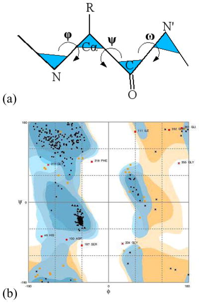
The density distribution of ϕ-ψ torsion angle pairs are plotted in a 2D plane. The correlation between the angle pairs is revealed in different density regions of the plot, with high correlations corresponding to high-density regions. The torsion angles ϕ, ψ, ω for a residue are indicated in (a). A sample Ramachandran Plot is displayed in (b).

Figure 2. Residue distances and angles.

(a) The α-τ-β angle triplet in a four-residue sequence. (b) The α-τ₁-β-τ₂-γ angle quintuplet in a five-residue sequence. The residues are assumed to be located at x_i, x_j, x_k, x_l, x_m.

With the increase in both the number and the quality of new protein structures, many structural properties can be derived from known protein structures by statistical analyses and data mining, and be used as a supplement to the experimental data for studies on structures. Indeed, the statistical measures on various types of residue distances and angles provide systematic and quantitative assessments of these properties, which can otherwise be estimated only individually and qualitatively. Their distributions and correlations in known protein structures reflect important aspects of protein structures, and offer insights into how proteins fold naturally into various residue-level structures.

Results

Distributions of residue distances

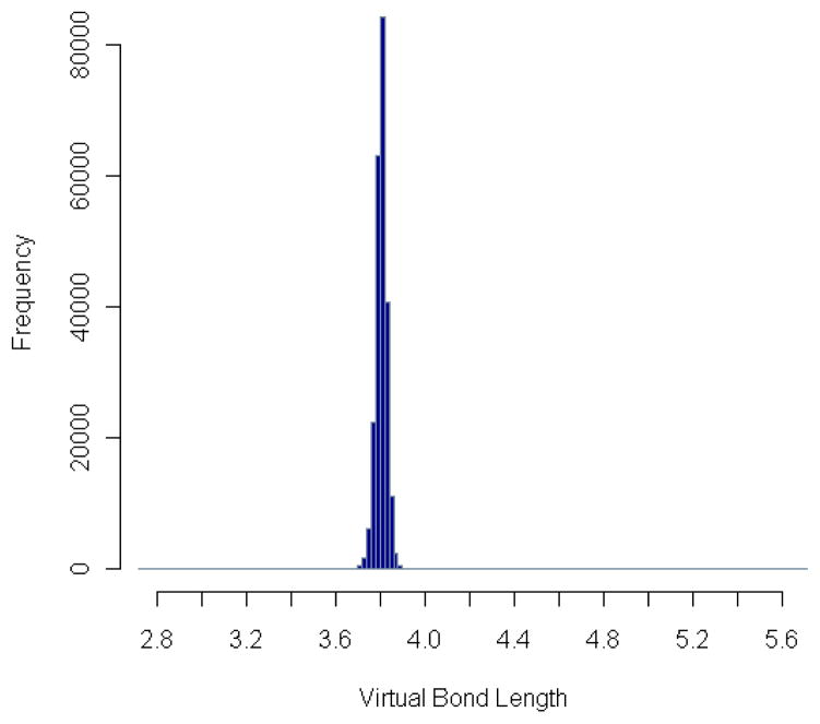
The residue-level virtual bond lengths or in other words, the residue-level, so-called 1–2-distances, for all the neighboring residue pairs in the downloaded protein structures are computed and accumulated. This data comprises the distribution of the virtual bond lengths over a range of distances (Fig. 3). The distributions of virtual bond lengths for specific residue pairs are also calculated and can be accessed through our R-package PRESS (see Additional Files).

Figure 3. Distribution of virtual bond length.

The residue-level 1–2-distances are grouped into small bins. The number of distances in each distance bin is plotted. The mean value of these distances is 3.80Å with standard deviation equal to 0.05Å.

The collected virtual bond lengths range from 2.73Å to 4.26Å, after removing a few large outliers (Table 1), but the average length is 3.80Å with a standard deviation equal to 0.05Å. This average length remains about the same for the residue pairs in α-helices or β-sheets, as shown in Fig. 4, where the number of distances between residue pairs in α-helices or β-sheets in each distance bin is plotted, and the two distributions are nearly the same as the general one in Fig. 3.

Table 1.

Sample virtual bond lengths

R1	#R1	R2	#R2	Length	Protein
GLU	345	GLU	346	2.7268Å	2ZWS
LYS	116	PRO	117	2.7564Å	2SNS
GLY	47	VAL	48	2.7647Å	2VOV
THR	4	GLU	5	2.7738Å	3ELN
GLY	8	GLY	9	2.7879Å	3F04
GLY	1001	GLU	1002	2.7920Å	2O9U
…
…
TRP	1092	ALA	1093	4.1051Å	1LU4
ALA	649	ASN	650	4.1497Å	1N7O
THR	276	GLU	277	4.2562Å	1GV9
LYS	292	LYS	293	4.9025Å	2VK2
LYS	195	TYR	196	5.5915Å	2BW4
ASN	263	PRO	264	9.3897Å	2JLI

The collected virtual bond lengths have been sorted. Shown here are the first and last six lengths listed (in Length), with their corresponding residue names (in R₁ and R₂), residue numbers (in #R₁ and #R₂), and protein ID (in Protein).

Figure 4. Distributions of virtual bond length in α-helices and β-sheets.

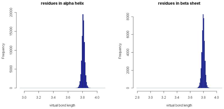
The number of distances between residue pairs in α-helices or β-sheets in each distance bin is plotted. The distributions are similar to the general one in Fig. 3. Note that a residue pair is counted as in α-helices or β-sheets if both residues are in α-helices or β-sheets.

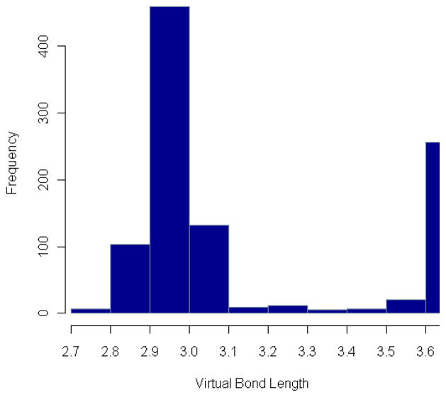
There is also a large number of short distances in the region from 2.7Å to 3.6Å, which are invisible in Figs. 3 and 4 because these are still relatively few compared to those greater than 3.6Å. However, when we look on a finer scale, we can see that they are concentrated around 2.9Å, forming another second peak in the distribution graphs (Fig. 5 and 6). The reason for the two peaks is that the four atoms C_α, C, N, C_α are always nearly planar but can exist in two forms: 1) the dominant trans structures with the distance between the two C_α atoms equal to 3.8Å approximately and 2) a few cis structures with the C_α-C_α distance around 2.9Å. To verify this, we have calculated the ω-angles of the residue pairs with distance < 3.1Å and > 3.1Å separately. The distributions of these angles (in Fig. 7) show that the angles corresponding to residue distances < 3.1Å are concentrated around 0° degree, while those corresponding to residue distances > 3.1Å are around 180°, which justifies our conjecture. However, it seems that the number of residue pairs with short residue distances (< 3.1Å) is quite small in α-helices or β-sheets (see Fig. 6). In fact, based on our calculated ω-angle values, there seem to be only a small number of residue pairs in α-helices or β-sheets having cis peptide bond structures, with only 5 in α-helices and 23 in β-sheets. Note that the distributions of the virtual bond lengths for specific pairs of residues can also be calculated and analyzed in the same way as above. They can be accessed through our R-package PRESS (see Additional Files). For example, among all types of residue pairs, the GLY-PRO pair has the smallest average distance, which is around 3.72Å with standard deviation equal to 0.26Å (because of the greater number of occurrences of cis peptide bonds). The distances for residue pairs with PRO as the second residue have a mean value smaller than 3.80Å with standard deviations ranging from 0.15Å to 0.30Å, which is about 3–6 times the standard deviation of the distances between general residue pairs. Interestingly, the distances formed by the residue pairs with PRO as the first residue do not have so much variation, providing an example where the distribution of the distances for a specific residue pair is not symmetric. This points up the much greater likelihood of the cis peptide bond immediately preceding PRO residues – a well-known fact.

Figure 5. Distribution of virtual bond length in short distance range.

The number of residue-level 1–2-distances in each distance bin is plotted over a short distance range. There is a small peak around 2.95Å.

Figure 6. Distributions of virtual bond length in α-helices and β-sheets in short distance range.

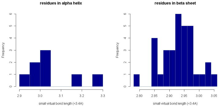
The number of residue-level 1–2-distances in α-helices and β-sheets in each distance bin is plotted in a short distance range.

Figure 7. Distributions of ω-angles for residue pairs.

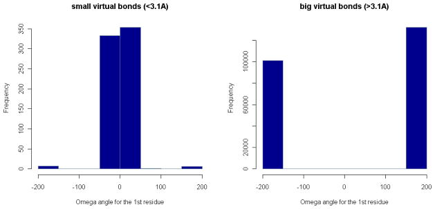
The angle interval [−180°, 180°] is divided into small bins. The number of ω-angles for residue pairs with distance < 3.1Å (or > 3.1Å) in each angle bin is plotted in the whole angle range.

Distributions of residue angles

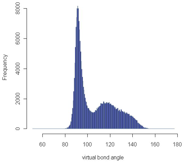
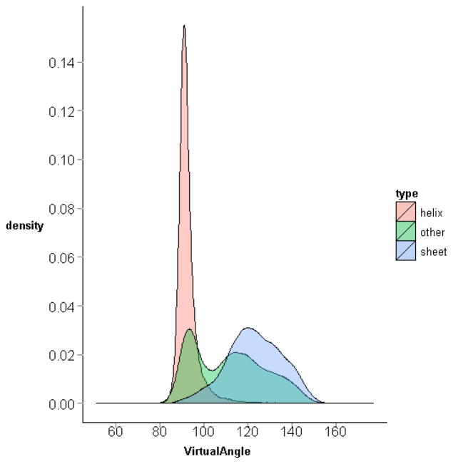
The residue-level virtual bond angles for all the three-residue sequences from the downloaded protein structures are computed and accumulated. The distribution of the virtual bond angles is shown in Fig. 8. The distributions of virtual bond angles for specific residue triplets have also been calculated and can be accessed through our R-package PRESS (see Additional Files). The collected virtual bond angles range from 51.3° to 177.0° as shown in Fig. 8, and have a distinct distribution when plotted separately for α-helices or β-sheets (Fig. 9). The sequential triplets in α-helices have an average virtual bond angle around 92.7° with a standard deviation of 5.37°, while those in β-sheets are somewhat more variable (standard deviation of 12.63°) with an average angle around 123.1°. Shown in Fig. 10 are the density plots for the virtual bond angles in α-helices, β-sheets, random coils in one graph. We see that the plots for the angles in α-helices and β-sheets form two large peaks. It further shows that the two large peaks in the general distribution plot in Fig. 8 are the sum of the angles in α-helices and β-sheets, respectively, which are due to the high frequency occurrences of the residue sequences in these two types of secondary structures in proteins. It is interesting to note however that the angles in other cases (random coils) seem to be distributed mostly in the same two large frequency peaks as well.

Figure 8. Distribution of virtual bond angle.

The residue-level virtual bond angles are grouped into small bins. The number of angles in each angle bin is plotted. Two frequency peaks around 90° and 120° respectively can be identified.

Figure 9. Distributions of virtual bond angle in α-helices and β-sheets.

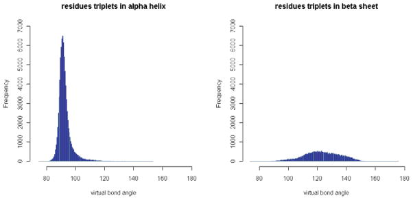
The number of angles for the residue triplets in α-helices or β-sheets in each angle bin is plotted. There are only single large peaks in each case. Note that a residue triplet is counted as in α-helices or β-sheets if the first and third residues are in α-helices or β-sheets.

Figure 10. Distributions of virtual bond angle in different secondary structures.

The densities of the virtual bond angles for the residue triplets in α-helices, β-sheets, and other random coils are plotted in one graph, with different colours. The density in α-helices is the highest, followed by that in β-sheets.

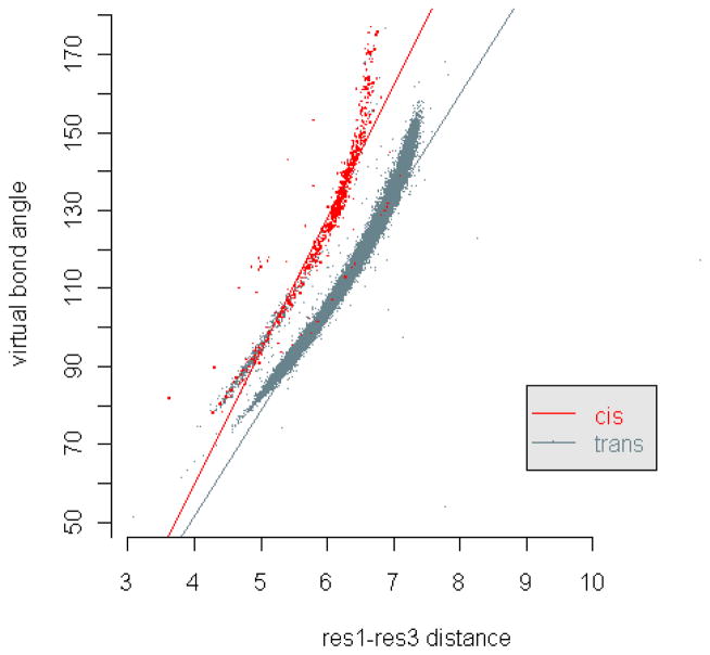
The residue-level 1–3-distance and the corresponding virtual bond angle for a three-residue sequence should agree with the cosine law: Let (R_i, R_i+1, R_i+2) be a sequence of three residues located at positions x_i, x_i+1, x_i+2 in R³. Let u = x_i+1 – x_i, v = x_i+2 – x_i+1. Then, the residue-level 1–3-distance for this sequence is d_i,i+2 = ||u + v|| = sqrt (||u||² + ||v||² – 2||u|·||v||·cosα), where α is the virtual bond angle of the sequence. However, if we treat the virtual bond lengths ||u|| and ||v|| as random variables, the correlation between the residue-level 1–3-distance and the corresponding virtual bond angle may not be identifiable clearly. Indeed, the correlations form two clearly separated curves as shown in Fig. 11, i.e., with a fixed distance, there may be two values of angles, and vice versa. The reason for this is that one of the virtual bonds in the residue triplets may form cis or trans structures with distinct bond lengths, resulting in different correlations between the residue-level 1–3-distance and the virtual bond angle. Indeed, when we examine all the distance-angle pairs in Fig. 11 and put a red point for each occurrence of a cis structure, we have found these points in the upper-left strip and the rest for trans structures in the right-most strip. Interestingly enough, for the trans cases there is a greater variability – generally the same angle value can be found for a wider range of distances or the same distance can be observed for a wider range of angles.

Figure 11. Correlation of residue-level 1–3-distance and virtual bond angle.

The residue-level 1–3-distances and the corresponding virtual bond angles are plotted as dots in a distance-angle plane. The red dots represent the distance-angle pairs with the corresponding residue triplets having a cis structure around one of their virtual bonds.

Distributions of residue torsion angles

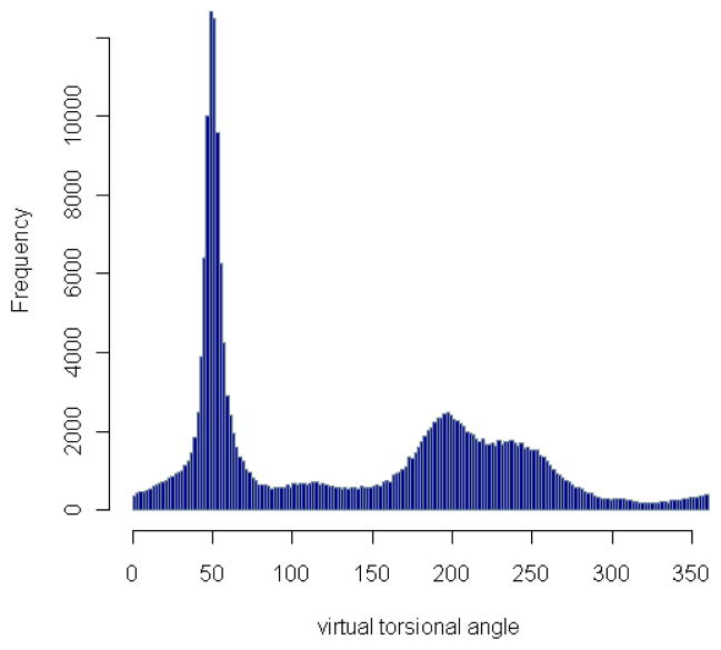
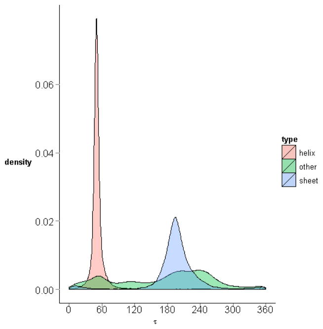
The residue-level virtual torsion angles for all four-residue sequences in the downloaded protein structures are computed and accumulated. The distribution of the virtual torsion angle over a large angle range is shown (Fig. 12). The distributions of virtual torsion angles for specific quadruplet of residues are also calculated and can be accessed through our R-package PRESS (see Additional Files). The collected virtual torsion angles have a range from 0° to 360°. The mean value is 137.6° with a standard deviation of 90.26°. Two high frequency peaks are observed: one around 55.9° corresponding to the residues in α-helices, and another around 195.2° corresponding to those in β-sheets. The peak for the virtual torsion angles formed by residues in α-helices exhibit less variability. If the distributions of virtual torsion angles are plotted for their occurrences in α-helices and β-sheets separately, there is then a single peak in each graph (Fig. 13). Each of these peaks corresponds to one of the two peaks seen in Fig. 12, suggesting that the two peaks in Fig. 12 are basically high frequency virtual torsion angles for the α-helices and β-sheets, respectively. The first peak occurs around 55.9°, which implies that the virtual torsion angles in α-helices are on average around 55.9°. The second peak is near 195.2°, meaning that the virtual torsion angles in β-sheets are around 195.2°. Figure 14 shows the density plots for the virtual torsion angles in α-helices, β-sheets, or other random coils in one graph. We see that the plots for the angles in α-helices and β-sheets form two large peaks. It further shows that the two large peaks in the general distribution plot in Fig. 12 should mainly be formed by the angles in α-helices and β-sheets, respectively, which correspond to the high frequency occurrences of the residue sequences in these two types of secondary structures in proteins. It is interesting to note though that the angles in other random coils seem to be distributed mostly in the two large frequency peaks as well, but unlike the virtual bond angles there are significant numbers of cases at intermediate values and even outside the α-helix and β-sheet peaks.

Figure 12. Distribution of virtual torsion angle.

The residue-level virtual torsion angles are grouped into small bins. The number of angles in each angle bin is plotted. Two peaks around 55.9° and 195.2° can be identified clearly in this plot.

Figure 13. Distributions of virtual torsion angle in α-helices and β-sheets.

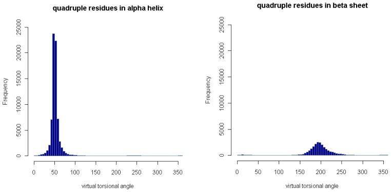
The number of angles for the residue quadruplets in α-helices or β-sheets in each angle bin is plotted. There are only single large peaks in both cases. Note that a residue quadruplet is counted as in α-helices or β-sheets if the first and third residues are in α-helices or β-sheets.

Figure 14. Distributions of virtual torsion angle in different secondary structures.

The densities of the virtual torsion angles for the residue quadruplets in α-helices, βsheets, and other random coils are plotted in one graph, with different colours. The density in α-helices is the highest, followed by that for β-sheets.

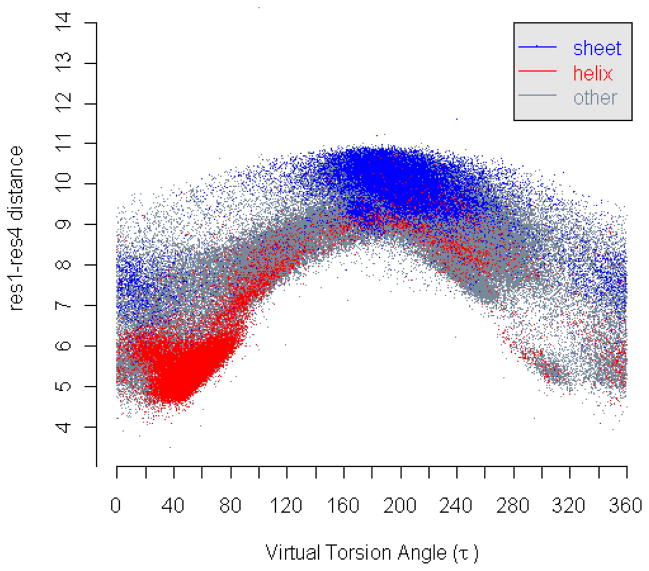
Let (R_i, R_i+1, R_i+2, R_i+3) be a sequence of four residues located at positions x_i, x_i+1, x_i+2, x_i+3 in R³. Let u = x_i+1 – x_i, v = x_i+2 – x_i+1, w = x_i+3 – x_i+2. Then, the residue-level 1–4-distance for this sequence is d_i,i+3 = ||u + v + w|| = sqrt (||u|| + ||v|| + ||w|| – 2||u||·||v||·cosα – 2||v||·||w||·cosβ – 2 ||u||·||w||·cosθ), where cosθ = sinα sinβ cosτ – cosα cosβ, and α, β, τ are virtual bond and torsion angles of this sequence. However, since the virtual bond lengths ||u||, ||v||, ||w||, and bond angles α, β are all random variables now, the correlation between the residue-level 1–4-distance and the corresponding virtual torsion angle may not be so clearly identifiable. Indeed, as shown in Fig. 15, one virtual torsion angle may correspond to multiple residue-level 1–4-distances, and vice versa. However, from 0° to 180°, the angle-distance pairs tend to concentrate from lower left to upper right, roughly forming a positive correlation between the residue 1–4-distances and their corresponding virtual torsion angles. From 180° to 360°, the pairs concentrate from upper left to lower right, forming a decreasing strip of dots. In either case, the residue 1–4-distances seems to be roughly correlated with their virtual torsion angles as shown by the above formula.

Figure 15. Correlation of residue-level 1–4-distance and virtual torsion angle.

The residue-level 1–4-distances and the corresponding virtual torsion angles are plotted as dots in a distance-angle plane. The blue dots represent the distance-angle pairs with the corresponding residue quadruplets in β-sheets while the red dots in α-helices.

Angle-angle correlations

The residue-level angle-angle correlations or, in other words, the correlations among the residue-level virtual bond angles and torsion angles in the downloaded protein structures are computed and documented. We exhibit, for sequences of angles, α-τ-β, the correlations between α-τ, τ-β, and α-β angle pairs and for sequences, α-τ₁-β-τ₂-γ, the correlations between τ₁-τ₂ angle pairs in Figs. 16–19. We form two large data sets, one containing all α-τ-β angle sequences and another containing all α-τ₁-β-τ₂-γ angle sequences. Each data set has 229,812 angle sequences. These are used to generate the density distributions of the angle-pairs (α-τ, τ-β, α-β, and τ₁-τ₂).

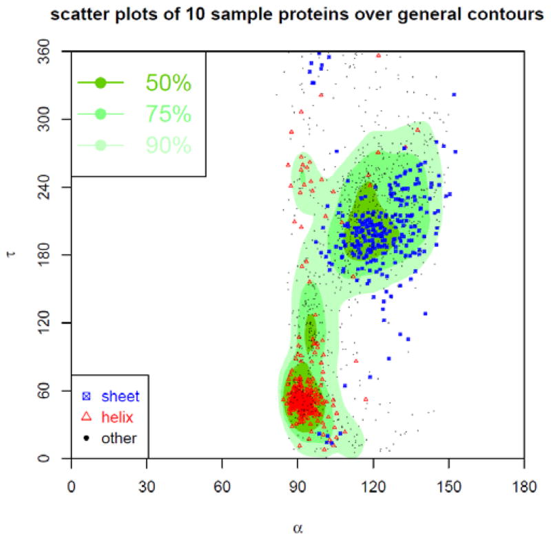
Figure 16. Contour of density distribution of α-τ angles pairs.

The contour of the density distribution of the α-τ angle-pairs is plotted. The plot is divided into three regions named as most favoured, favoured, and allowed, each containing high 50%, 75%, and 90% of all α-τ angle pairs. In addition, the α-τ angle pairs sampled from 10 arbitrarily selected proteins are plotted as points. The red triangles represent the α-τ angle-pairs in α-helices, the blue squares in β-sheets, and the black dots in other type of secondary structures.

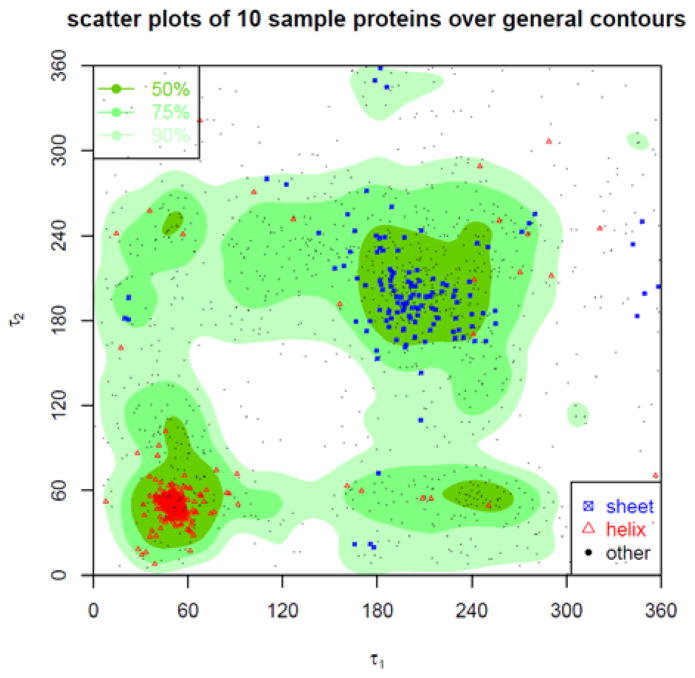
Figure 19. Contour of density distribution of τ₁-τ₂ angle pairs.

The contour of the density distribution of the τ₁-τ₂ angle pairs is plotted. The plot is divided into three regions named as most favoured, favoured, and allowed, each containing high 50%, 75%, 90% of all the τ₁-τ₂ angle pairs. In addition, the τ₁-τ₂ angle pairs sampled from 10 arbitrarily selected proteins are plotted as dots overlaid on the contour of the general τ₁-τ₂ density distributions. The red triangles represent the τ₁-τ₂ angle-pairs in α-helices, the blue squares in β-sheets, and the black dots in other type of secondary structures.

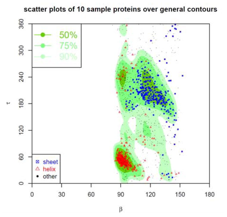
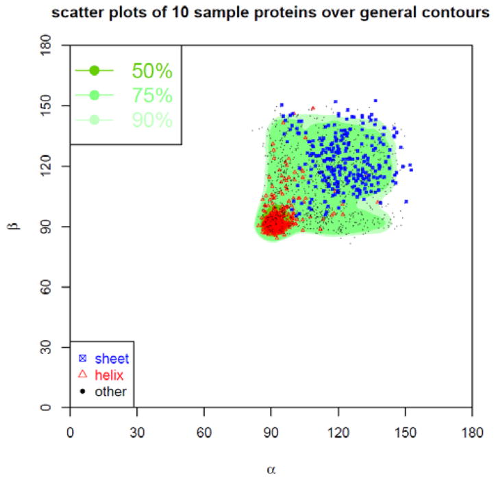
The background plots in Fig. 16–19 are the contours of the density distributions of the angle pairs. The scattered dots correspond to the angle pairs found in 10 sampled protein structures. The background contours are plotted in different gradients, with a darker gradient representing higher density regions. From high to low density, there are 50%, 75%, and 90% density regions, named Most Favoured, Favoured, and Allowed regions, respectively. The plots show that there are distinct density distribution regions for α-τ and τ-β angle pairs. That means that these angle pairs are highly dependent of each other in well-formed protein structures or in other words, if one angle in α-τ or τ-β angle pair is fixed, the choice for the other is restricted. These correlations are certainly important structural properties of proteins, but have not been investigated thoroughly. However, for α-β and τ₁-τ₂ angle pairs, the correlations are not so strong: One angle does not impose as strong a restriction on the possible choices for the other. The scattered dots for the angle pairs from 10 sampled structures further confirm the correlations of the angle pairs reflected in the general estimations, i.e., the distributions of the angle pairs in these structures (represented by the dots) agree with those in all the downloaded structures (represented by the background contours). We have also used two differently coloured dots for the angle pairs in α-helices and β-sheets, respectively. Then, the differently coloured dots are distributed in different high-density regions. The following are more specific explanations of the plots.

The contour of the density distribution of α-τ angle pairs is plotted in Fig. 16. The contour is displayed in three types of regions named as Most Favoured, Favoured, and Allowed, each containing high 50%, 75%, 90% of all collected α-τ angle pairs. In addition, the α-τ angle pairs sampled from 10 arbitrarily selected proteins are overlaid as points over the contour of the general α-τ density distribution. The red triangles represent the α-τ angle-pairs in α-helices, the blue squares in β-sheets, and the black dots in other type of secondary structures. In total 1756 scattered points for the sampled structures (PDB ID: 1TJY, 1UJP, 1WCK, 2BOG, 2DSX, 2E3H, 2FG1, 2O8L, 2P4F, 3IIS) are shown, of which 1566 points (~89.2%) are in Allowed regions, 1319 points (~75.1%) in Favoured regions, and 901 points (~51.31%) in Most Favoured regions. Table 2 shows the percentile of α-τ angle pairs in Allowed, Favoured, and Most Favoured regions for each of the 10 sampled protein structures. Most of these proteins, especially the proteins with more helical structures such as 3IIS, have high percentages of points in these regions, but 2E3H, with no helical structures, is an exception.

Table 2.

Density distribution of α-τ angle pairs

Protein ID	Allowed region	Favoured region	Most Favoured region
1TJY	91.37%	75.72%	55.59%
1UJP	93.51%	80.09%	63.20%
1WCK	83.46%	65.41%	29.32%
2BOG	86.50%	72.99%	52.19%
2DSX	95.92%	73.47%	38.78%
2E3H	80.00%	62.67%	22.67%
2FG1	82.22%	68.15%	48.89%
2O8L	84.51%	68.15%	33.33%
2P4F	94.59%	87.57%	60.00%
3IIS	96.62%	89.86%	77.70%

The table gives the percentiles of α-τ angle pairs in the allowed, favoured, and most favoured regions of the general α-τ density distribution contour for 10 sampled protein structures.

The density distribution contour of τ-β angle-pairs is plotted in Fig. 17. The contour is displayed in three types of regions named as Most Favoured, Favoured, and Allowed regions, each containing high 50%, 75%, and 90% of all collected τ-β angle pairs. In addition, the τ-β angle pairs sampled from the same 10 arbitrarily selected proteins are plotted as points on top of the contour of the general τ-β density distribution. The red triangles represent the τ-β angle pairs in α-helices, the blue squares in β-sheets, and the black dots in other type of secondary structures. In total 1756 scattered points from the same sampled structures are shown, of which 1567 points (~89.8%) are in Allowed regions, 1338 points (~76.2%) in Favoured regions, and 941 points (~53.59%) in Most Favoured regions. Table 3 gives the percentile of τ-β angle pairs in Allowed, Favoured, and Most Favoured regions for each of 10 sampled protein structures. Most of these proteins, especially the proteins with more helical structures, have high percentages of points in these regions, while proteins 2E3H and 1WCK with more sheets have lower percentiles of points in these regions than average. The density distribution contour of α-β angle-pairs is plotted in Fig. 18, with regions also named as Most favoured, Favoured, Allowed, each corresponding to high 50%, 75%, 90% of all collected α-β angle pairs. In addition, the α-β angle pairs sampled from the 10 arbitrarily selected proteins are plotted as points on top of the contour of the general α-β density distribution. The red triangles represent the α-β angle-pairs in α-helices, the green squares in β-sheets, and the black dots in other type of structures. In total 1756 scattered points for the same sampled structures are shown, of which 1681 points (~95.7%) are in Allowed regions, 1608 points (~91.6%) in Favoured regions, and 645 points (~36.73%) in Most Favoured regions.

Figure 17. Contour of density distribution of τ-β angles pairs.

The contour of the density distribution of the τ-β angle-pairs is plotted. The plot is divided into three regions named as most favoured, favoured, and allowed, each containing 50%, 75%, and 90% of all τ-β angles-pairs. In addition, the τ-β angle pairs sampled from 10 arbitrarily selected proteins are also plotted as points on top of the contour of the general τ-β density distribution. The red triangles represent the τ-β angle pairs in α-helices, the blue squares in β-sheets, and the black dots in other type of secondary structures.

Table 3.

Density distribution of τ-β angle pairs

Protein ID	Allowed region	Favoured region	Most Favoured region
1TJY	91.37%	77.96%	56.55%
1UJP	93.51%	85.71%	66.23%
1WCK	81.95%	70.68%	36.09%
2BOG	87.23%	73.72%	52.55%
2DSX	97.96%	81.63%	40.82%
2E3H	77.33%	56.00%	30.67%
2FG1	90.37%	73.33%	51.85%
2O8L	84.98%	64.32%	36.62%
2P4F	94.59%	84.32%	61.62%
3IIS	96.62%	85.14%	77.03%

The table gives the percentiles of τ-β angle pairs in the allowed, favoured, and most favoured regions of the general τ-β density distribution contour for 10 sampled protein structures.

Figure 18. Contour of density distribution of α-β angle pairs.

The contour of the density distribution of the α-β angle pairs is plotted. The plot is divided into three regions named as most favoured, favoured, and allowed, each containing high 50%, 75%, and 90% of all α-β angle pairs. In addition, the α-β angle pairs sampled from 10 arbitrarily selected proteins are plotted as dots over the contour of the general α-β density distribution. The red triangles represent the α-β angle pairs in α-helices, the blue squares in β-sheets, and the black dots in other type of secondary structures.

The density distribution contour of τ₁-τ₂ angle pairs is plotted in Fig. 19, with regions again named as Most favoured, Favoured, Allowed, each corresponding to high 50%, 75%, 90% of all collected τ₁-τ₂ angle pairs. In addition, the τ₁-τ₂ angle pairs sampled from the same 10 selected proteins are plotted as points on top of the contour of the general τ₁-τ₂ density distribution. The red triangles represent the τ₁-τ₂ angle pairs in α-helices, the blue squares in β-sheets, and the black dots in other type of secondary structures. In total there are 1737 scattered points for the sampled structures, of which 1551 points (~89.3%) are in Allowed regions, 1309 points (~75.4%) in Favoured regions, and 902 points (~51.93%) in Most Favoured.

Applications to structural analysis

The distributions of residue-level virtual bonds, bond angles, and torsion angles can be used to define residue-level statistical potentials. The energy distributions over sequences of virtual bond lengths, virtual bond angles, or virtual torsion angles for a given protein structure can then be evaluated with corresponding potential energy functions. If the potential energy is high for a virtual bond length (or a virtual bond angle or a virtual torsion angle), it implies that the virtual bond length (or the virtual bond angle or the virtual torsion angle) is not energetically favourable.

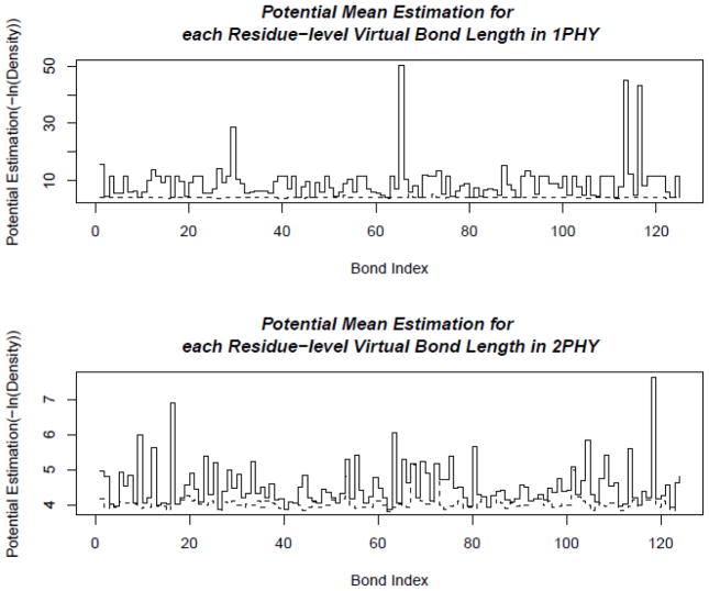
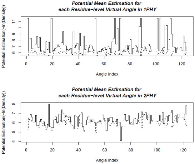
The density distributions of α-τ and τ-β angle pairs show strong correlations. Therefore, a given structure can also be evaluated by comparing its α-τ and τ-β angle pairs with their general distributions. A 2D plot can be obtained by positioning these angle pairs, as points, in the corresponding 2D contours of their general density distribution functions. The 2D contours have three density regions, called Most Favoured, Favoured, and Allowed, corresponding to high 50%, 75%, and 90% of all the angle pairs in the surveyed structures. A structure is considered to be well-formed in terms of its α-τ (or τ-β) angle pairs if the percentiles of the α-τ (or τ-β) angle pairs falling in the corresponding density regions are close to their general distributions. Figs. 20–25 show how the statistical potentials and the angle correlation plots can be used for structural analysis, for example, how they can be used effecively for distinguishing a well-resolved structure from a poorly determined one. In these figures, we see that the energy distributions along the residue sequences for two structures of different resolutions are clearly different. The potential energies for the better resolved structure are lower in average. The distributions of the α-τ or τ-β angle pairs of the structures show even greater contrast. The better resolved structure has many more angle pairs distributed in the high density regions of the corresponding angle distribution contour, while the poorly resolved structures have many angle pairs falling outside of these high density regions.

Figure 20. Distributions of virtual bond energies for 1PHY (2.4 Ǻ) and 2PHY (1.4 Ǻ).

The energy levels of the virtual bond lengths of two structures 1PHY and 2PHY are shown in solid lines. The minimal possible energies are plotted as the dashed line. If there is no distribution data for some virtual bond, such as the bond at index 98, the potential function is not defined, and there is a gap in the energy plot for that bond. These two structures are determined with different resolutions for the same protein. The better-resolved structure (2PHY) has lower potential energies in average than the poorly determined one (1PHY).

Figure 25. τ-β correlation plots for 1PTE (2.8Ǻ) and 3PTE (1.6Ǻ).

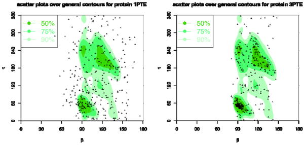
The background plots are the contours of the general density distributions of τ-β angle pairs coloured with different levels of density to indicate high 50% (most favoured), 75% (favoured), and 90% (allowed) regions. The dots correspond to the τ-β angle pairs for the given protein structures. The plot for 1PTE has only 55.35%, 33.33%, and 14.68% angle pairs in allowed, favoured, and most favoured regions, respectively, while 3PTE has 89.24%, 77.03%, and 52.33% angle pairs in those regions.

More specifically, in Fig. 20, we show the energy levels of virtual bond lengths of two structures, 1PHY and 2PHY. They are two structures determined at two different times for the same photoreactive yellow protein. 1PHY has a lower quality (2.4Ǻ) now replaced by 2PHY with 1.4Å resolution. As we can see, the better-resolved structure (2PHY) has certainly lower virtual bond energies in average than the poorly determined one (1PHY). In Fig. 21, we see the energy levels of the virtual bond angles of the structures. Again, the better-resolved structure (2PHY) has lower virtual bond angle energies than the poorly determined one (1PHY).

Figure 21. Distribution of virtual bond angle energies for 1PHY (2.4 Ǻ) and 2PHY (1.4 Ǻ).

The energy levels of the virtual bond angles of two structures 1PHY and 2PHY are plotted in solid lines. The minimal possible energies are shown as the dashed line. These two structures are determined with different resolutions for the same protein. The better-resolved structure (2PHY) has lower potential energies in average than the poorly determined one (1PHY).

In Fig. 22, we show the α-τ plots for structures 1PHY vs. 2PHY. The plot for 1PHY has only 51.22%, 28.46%, and 10.57% angle pairs in Allowed, Favoured, and Most Favoured regions, respectively, while 2PHY has 93.44%, 76.23%, and 45.9% angle pairs in these regions. In Fig. 23, we show the τ-β plots for structures 1PHY vs. 2PHY. The plot for 1PHY has only 58.54%, 33.33%, and 13.82% angle pairs in Allowed, Favoured, and Most Favoured regions, respectively, while 2PHY has 95.9%, 75.41%, and 47.54% angle pairs in these regions.

Figure 22. α-τ correlation plots for 1PHY (2.4Ǻ) and 2PHY (1.4Ǻ).

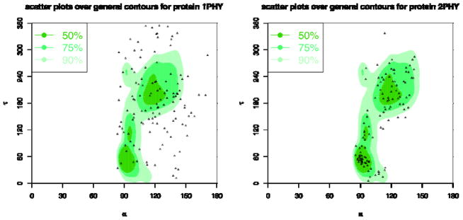
The background plots are the contours of the general density distributions of α-τ angle pairs coloured with different levels of density to indicate high 50% (most favoured), 75% (favoured), and 90% (allowed) regions. The dots correspond to the α τ angle pairs in the given protein structures. The plot for 1PHY has only 51.22%, 28.46%, and 10.57% angle pairs in allowed, favoured, and most favoured regions, respectively, while 2PHY has 93.44%, 76.23%, and 45.9% angle apirs in those regions.

Figure 23. α-τ correlation plots for 1PTE (2.8Ǻ) and 3PTE (1.6Ǻ).

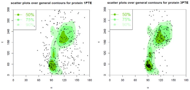
The background plots are the contours of the general density distributions of α-τ angle pairs coloured with different levels of density to indicate high 50% (most favoured), 75% (favoured), and 90% (allowed) regions. The dots correspond to the α τ angle pairs in the given protein structures. The plot for 1PTE has only 45.87%, 28.75%, and 14.68% angle pairs in allowed, favoured, and most favoured regions, respectively, while 3PTE has 89.24%, 73.84%, and 49.13% angle apirs in those regions.

In Fig. 24, we further show the α-τ plots for structures 1PTE vs. 3PTE for the same DD-peptidase penicillin-target enzyme. 1PTE has a resolution of 2.8Ǻ now replaced by 3PTE with 1.6Å resolution. The plot for 1PTE has only 45.87%, 28.75%, and 14.68% angle pairs in Allowed, Favoured, and Most Favoured regions, respectively, while 3PTE has 89.24%, 73.84%, and 49.13% angle pairs in these regions. In Fig. 25, we show the τ-β plots for structures 1PTE vs. 3PTE. The plot for 1PTE has only 55.35%, 33.33%, and 14.68% angle pairs in Allowed, Favoured, and Most Favoured regions, respectively, while 3PTE has 89.24%, 77.03%, and 52.33% angle pairs in these regions. These results demonstrate that the α-τ and τ-β plots can clearly be used to distinguish between high and low-quality structures, and may be extended for use in practice as residue-level Ramachandran Plots for structural analysis and refinement.

Figure 24. τ-β correlation plots for 1PHY (2.4Ǻ) and 2PHY (1.4Ǻ).

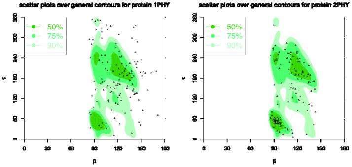
The background plots are the contours of the general density distributions of τ-β angle pairs coloured with different levels of density to indicate high 50% (most favoured), 75% (favoured), and 90% (allowed) regions. The dots correspond to the τ-β angle pairs for the given protein structures. The plot for 1PHY has only 58.54%, 33.33%, and 13.82% angle pairs in allowed, favoured, and most favoured regions, respectively, while 2PHY has 95.9%, 75.41%, and 47.54% angle pairs in those regions.

Discussion

The statistical distributions of residue-level distances and angles in known protein structures provide a valuable source of information for estimating these residue level structural properties of proteins, which are not otherwise accessible experimentally. However, these statistical measures rely upon the quality as well as quantity of the sampled known structures. We have downloaded around one thousand high-quality structures from the PDB Data Bank, which should be sufficient to obtain reliable statistical estimates of the distributions of virtual bond lengths, virtual bond angles, virtual torsion angles, and some of their correlations, but of course there is the possibility that for some cases of specific residue sequences, the values might deviate from the overall characteristic distributions. In our software PRESS, we have provided information about the size of the data set for each estimate.

One of the most important results from this study shows that residue-level angles, especially the neighboring virtual bond angles and virtual torsion angles, exhibit strong correlations. For example, if a virtual bond angle is fixed, then the choice for the virtual torsion angle adjacent to it will be highly restricted. Such a correlation is similar to the correlation shown in Ramachandran Plots between the backbone atomic ϕ-ψ torsion angles, and can be equally important for understanding the structural properties of proteins at their residue-levels and even for evaluating the quality of individual structures. However, as we have shown, the correlations between two virtual bond angles, when separated by one virtual torsion angle, are not so strong, and so are the correlations between two virtual torsion angles, when separated by one virtual bond angle. The reason may be due to the fact that at residue-level, these angles are relatively further apart and therefore behave more independently of one another. In addition, where the angles are closely correlated, they tend to have smaller deviations when they are in α-helices than in β-sheets. This implies that even at the residue-level, α-helices are more rigid (or stable) than β-sheets.

We have demonstrated that the statistical distributions of the residue-level distances or angles can be used to define various statistical potentials, but further refinements are required to make them computationally and physically meaningful. For example, the potentials for virtual bond lengths of different pairs of residues, or for virtual bond angles of different triplets of residues, or for virtual torsion angles of different sequence quadruplets of residues, need to be scaled appropriately before they can be combined. These are only potentials for short-range interactions. In order to define a relatively complete energy function for a protein, potentials for long-range interactions also must be included.

The useful tool from this study is a residue-level Ramamchandran-type of plot for correlations between pairs of neighboring virtual bond angles and virtual torsion angles. Several examples have been given in the present paper, but these differ from the atomic-level Ramachandran Plot in an important way, because the density distribution contours of these residue-level angles show relatively larger deviations. Thus their use requires specifying more precisely what density regions should be permitted for high-quality structures. Further evaluations are needed to decide generally what these evaluation criteria should be.

Conclusions

The atomic-level structural properties of proteins, such as bond lengths, bond angles, and torsion angles, have been thoroughly studied and understood based on either chemistry knowledge or statistical analysis. Similar properties at the residue-level, such as the distances between two residues and the angles formed by short sequences of residues, can be equally important for structural analysis and modelling, but these have not previously been examined and tabulated as carefully and thoroughly. While these properties are difficult to measure experimentally, they can be estimated statistically based on observed distributions in known proteins structures, as demonstrated in this paper.

In this paper, we have conducted a statistical analysis of protein residue-level local structural properties. A software package was built, and this provides direct access to the statistical data for these properties including correlations among them. The distributions of residue distances and angles may vary residue sequence, but in most cases, these are concentrated in some high probability ranges, which correspond to their frequent occurrences in either α-helices or β-sheets in proteins. Strong correlations among neighbouring residue angles, similar to those between neighbouring torsion angles at the atomic-level, are revealed based on statistical measures. Residue-level statistical potentials can be defined using the statistical distributions and correlations of the residue distances and angles. Ramachandran-like plots for strongly correlated residue angles are plotted and analyzed. Their applications for structural evaluation and refinement are demonstrated.

With the increase in both the number and quality of determined protein structures, many structural properties can be derived from known protein structures with statistical analysis and data mining, and then be used as a supplement to experimental data for refining or evaluating structures. Indeed, the statistical measures of various types of residue distances and angles afford systematic and quantitative assessments on these properties. Their distributions and correlations in known protein structures inform us about the important limitations of conformations of proteins and can even offer some insights into how proteins fold or change their conformations.

Methods

Selection of known protein structures

1052 X-ray crystallography structures were downloaded from the PDB Data Bank [21], with resolution ≤ 1.5 Å, sequence similarity ≤ 30%, and only single chains. NMR structures are excluded since they are usually represented as ensembles of structures, with part of the structure being built from computational modelling, which would introduce uncontrollable biases into our evaluations. We could have selected a representative structure from each ensemble, say the average or energy minimized one [22], but we decided to use only X-ray crystallography structures in this work. By limiting the resolution to be 1.5 Å or better, the structures are guaranteed to be quite accurate but yet have sufficient numbers of structures for conducting statistical analysis. By excluding proteins having sequence similarity above 30%, redundancies are removed, and structures are less likely to be repeated and hence over sampled. Multi-chain structures are often multi-copies of single chains, and are also excluded as well to avoid the duplication in the data.

Calculation of residue distances and angles

The position of the C_α atom is used to define the position of a residue. The distance between two C_α atoms is used to represent the distance between two residues. We call the distance between two neighboring residues a virtual bond. Two connected virtual bonds, sharing the central residue, form a virtual bond angle. Three connected virtual bonds make a torsion angle - a virtual torsion angle (Fig. 2). We also call the distance between the two adjacent residues in a sequence the residue-level 1–2-distance, between the first and third a residue-level 1–3-distance, the first and fourth a residue-level 1–4-distance, and so forth. Three residues in sequence form a virtual bond angle. Four residues in sequence have two virtual bond angles with a virtual torsion angle between them. We identify these as α, τ, β, respectively, where τ is the virtual torsion angle. Five residues in sequence have three virtual bond angles with two virtual torsion angles separating them. We call them α, τ₁, β, τ₂, γ angles, respectively, where τ₁ and τ₂ are the virtual torsion angles.

For each of the downloaded structures, there are n-1 pairs of neighboring residues (R_i, R_i+1), i = 1, …, n-1, or virtual bonds, where n is the total number of residues in the structure; similarly, there are n-2 sequences of three residues (R_i, R_i+1, R_i+2), i = 1, …, n-2, or virtual bond angles and n-3 sequences of four residues (R_i, R_i+1, R_i+2, R_i+3), i = 1, …, n-3, or virtual torsion angles, and n-4 sequences of five residues (R_i, R_i+1, R_i+2, R_i+3, R_i+4), i = 1, …, n-4. For each of the downloaded structures, the residue-level 1–2-distances for all n-1 neighboring residue pairs, the residue-level 1–3-distances for all n-2 sequences of three residues, and the residue-level 1–4-distances for all n-3 sequences of four residues are calculated and accumulated in three separate files. For all n-2 three-residue sequences, their virtual bond angles are calculated and saved. For all n-3 four-residue sequences, their α, τ, β angles are calculated and tabulated. For all n-4 five-residue sequences, their α, τ₁, β, τ₂, γ angles are calculated and saved. Let (R_i, R_i+1) be a sequence of two residues located at positions x_i and x_i+1 in R³. Let the difference in positions i +1 and i be u = x_i+1 – x_i. Then, the residue-level 1–2-distance for this sequence is d_i,i+1 = ||u||, where ||·|| is the Euclidean norm, ||u|| = sqrt (u₁² + u₂² + u₃²) for any u = (u₁, u₂, u₃)^T in R³. Let (R_i, R_i+1, R_i+2) be a sequence of three residues located at positions x_i, x_i+1, x_i+2 in R³. Let u = x_i+1 – x_i, v = x_i+2 – x_i+1. Then, the residue-level 1–3-distance for this sequence is d_i,i+2 = ||u + v|| = sqrt (||u||² + ||v||² – 2||u|·||v||·cosα), where α is the virtual bond angle of this sequence. Let (R_i, R_i+1, R_i+2, R_i+3) be a sequence of four residues located at positions x_i, x_i+1, x_i+2, x_i+3 in R³. Let u = x_i+1 – x_i, v = x_i+2 – x_i+1, w = x_i+3 – x_i+2. Then, the residue-level 1–4-distance for this sequence is d_i,i+3 = ||u + v + w|| = sqrt (||u|| + ||v|| + ||w|| – 2||u||·||v||·cosα – 2||v||·||w||·cosβ – 2 ||u||·||w||·cosθ) , where cosθ = sinα sinβ cosτ – cosα cosβ, and α, β, τ are virtual bond and torsion angles of this sequence.

Calculation of distance and angle distributions

For any two-residue sequence, the sequence together with their corresponding 1–2-distances from all the downloaded structures can be found in the residue-level 1–2-distance files. Similarly, for any three-residue sequence, the same sequence and its 1–3-distances from all the downloaded structures can be found in the residue-level 1–3-distance files; and for any four-residue sequence, this sequence and its 1–4-distances from all the downloaded structures can be found in the residue-level 1–4-distance files. For each of these distance types, a density distribution of the distances can be found with the collected distances. A distance interval is divided into small bins. The density distribution of a distance in any of these bins is defined as the number of distances in that bin divided by the total number of distances in the distance interval (see Fig. 3).

For any three-residue sequence, its corresponding virtual bond angles from all the downloaded structures can be found in the bond angle files. Similarly, for any four-residue sequence, the same sequence and its virtual torsion angles occurring in all the downloaded structures can be found in the virtual torsion angle files. For each of these angle types, a density distribution of the angles can be found using the collected angles. A 180º angle interval is divided into small bins for the virtual bond angles, and a 360º angle interval is divided into small bins for the virtual torsion angles. The density distribution of an angle in any of these bins is defined as the number of angles in that bin divided by the total number of angles in the angle interval (see Figs. 8 and 12).

Calculation of angle-angle and angle-distance correlations

All four-residue sequences and their α-τ-β angles in all the downloaded structures can be found in the virtual torsion angle files. The density distribution of the α-τ-β angles can be found by using the collected angle sequences. The 180º angle interval for α is divided into small bins. A 360º angle interval for τ is divided into small bins. A 180º angle interval for β is divided into small bins. Multiply these intervals to form a subspace [0º, 180º]×[0º, 360º]×[0º, 180º] in R³, which is divided into small boxes. The density distribution of a sequence of α-τ-β angles in any of these boxes is defined as the number of the angle sequences in that box divided by the total number of the angle sequences in the entire angle subspace.

All five-residue sequences and their α-τ₁-β-τ₂-γ angles in all the downloaded structures can be found in the virtual torsion angle files. The density distribution of τ₁-β-τ₂ angles can be found by using the collected angle sequences. A 360º angle interval for τ₁ is divided into small bins. An 180º angle interval for β is divided into small bins. A 360º angle interval for τ₂ is divided into small bins. Multiplying these intervals together forms a subspace [0º, 360º]×[0º, 180º]×[0º, 360º] in R³, which is divided into small boxes. The density distribution of a sequence of τ₁-β-τ₂ angles in any of these boxes is defined as the number of the angle sequences in that box divided by the total number of the angle sequences in the entire angle subspace. Two special density distributions are calculated: the density distributions of the α-τ angles and the τ-β angles in the α-τ-β angle sequences. These are simply the projections of the α-τ-β density distribution on the α-τ and τ-β subspaces, but they demonstrate more clearly the correlations of the angles. The density distribution of α-β angle pairs in α-τ-β angle sequences and τ₁-τ₂ angle pairs in τ₁-β-τ₂ angle sequences have also been calculated. All these density distributions are plotted in a 2D plane for the corresponding two angles (see Figs. 16–19).

For all three-residue sequences, their virtual bond angles and corresponding 1–3-distances from all the downloaded structures can be found in the virtual bond angle files and the residue-level 1–3-distance files. The correlations between the virtual bond angles and their corresponding 1–3-distances can be demonstrated using the density distributions of the virtual bond angles compared to their corresponding 1–3-distances in an angle-distance space. An 180º angle interval is divided into small bins for the virtual bond angles. A 20Å distance interval is divided into small bins for the corresponding 1–3-distances. Multiply the angle interval with the distance interval to obtain the subspace [0º, 180º]×[0Å, 20Å] in R². The subspace is divided into small squares. The density of the angle-distance pairs in each of these squares is defined as the number of the angle-distance pairs in that square divided by the total number of angle-distance pairs in the entire angle-distance subspace (see Fig. 11).

For all four-residue sequences, their virtual torsion angles and corresponding 1–4-distances in all the downloaded structures can be found in the virtual torsion angle files and the residue-level 1–4-distance files. The correlations between the virtual torsion angles and their corresponding 1–4-distances can be demonstrated using the density distributions of the virtual torsion angles vs. their corresponding 1–4-distances in angle-distance space. A 360º angle interval is divided into small bins for the virtual torsion angles. A 20Å distance interval is divided into small bins for the corresponding 1–4-distances. Multiply the angle interval with the distance interval to obtain a subspace [0º, 360º]×[0Å, 20Å] in R². Then the subspace can be divided into small squares. The density of the angle-distance pairs in each of these squares is defined as the number of the angle-distance pairs in that square divided by the total number of angle-distance pairs in the entire angle-distance subspace (see Fig. 15).

Definition of residue distance and angle potentials

The density distribution functions for the virtual bond lengths, virtual bond angles, and virtual torsion angles are approximated with Gaussian kernels. Let P[R_i, R_i+1](D_i,i+1) be the density distribution function for the distance D_i,i+1 between residues R_i and R_i+1. A potential energy function for this distance can be defined as E[R_i, R_i+1](D_i,i+1) = – kT ln P[R_i, R_i+1](D_i,i+1), where k is the Boltzmann constant and T a temperature factor. Let P[R_i, R_i+1, R_i+2](A_i,i+1,i+2) be the density distribution function for the angle A_i,i+1,i+2 formed by residues R_i, R_i+1, R_i+2. The potential energy function for this angle can be defined as E[R_i, R_i+1, R_i+2](A_i,i+1,i+2) = – kT ln P[R_i, R_i+1, R_i+2](A_i,i+1,i+2). Let P[R_i, R_i+1, R_i+2, R_i+3](T_{i,i+1,i+2,i+3}) be the density distribution function for the torsion angle T_{i,i+1,i+2,i+3} formed by residues R_i, R_i+1, R_i+2, R_i+3. The potential energy function for this angle can be defined as E[R_i, R_i+1, R_i+2, R_i+3](T_{i,i+1,i+2,i+3}) = – kT ln P[R_i, R_i+1, R_i+2, R_i+3](T_{i,i+1,i+2,i+3}). With these potential energy functions, the distributions of the virtual bond length potentials, virtual bond angle potentials, and virtual torsion angle potentials can be calculated and displayed for a given structure over its residue sequence (see Figs. 20–21).

Display of residue angle correlations of a structure

The contours of density distributions of α-τ and τ-β angle pairs are plotted in 2D α-τ and τ-β angle planes. Regions of different densities are outlined with colours of different gradients. They are defined as Most Favoured, Favoured, and Allowed, corresponding to regions of high 50%, 75%, and 90% density, respectively. The α-τ or τ-β angle pairs for every sequence of four residues of a given structure can be computed and plotted in the α-τ or τ-β plane, on top of the contour of the general α-τ or τ-β density distribution function. The structure is considered to be well formed in terms of its virtual bond angles and virtual torsion angles if the percentiles of the plotted dots in the corresponding density regions of the contour are close to the general distributions of the angle pairs in these regions (see Figs. 22–25).

Figure 26. PRESS graphics interface.

PRESS has a graphical interface with six functional panels corresponding to six functional routine, each providing a specific structural computing or analysis function.

References

- 1.Creighton TE. Proteins: Structures and Molecular Properties. 2. Freeman and Company; 1993. [Google Scholar]
- 2.Dunbrack RL. Rotamer libraries in the 21st century. Curr Opin Struct Biol. 2002;12:431–440. doi: 10.1016/s0959-440x(02)00344-5. [DOI] [PubMed] [Google Scholar]
- 3.Brooks CL, III, Karplus M, Pettitt BM. Proteins: A Theoretical Perspective of Dynamics, Structure, and Thermodynamics. Wiley; 1989. [Google Scholar]
- 4.Schlick T. Molecular Modeling and Simulation: An Interdisciplinary Guide. Springer; 2003. [Google Scholar]
- 5.Wüthrich K. NMR in Structural Biology. World Scientific Publishing Company; 1995. [Google Scholar]
- 6.Laskowski RA, MacArthur MW, Moss DS, Thornton JM. PROCHECK: a program to check the stereochemical quality of protein structures. Journal of Applied Crystallography. 1993;26:283–291. [Google Scholar]
- 7.Bernasconi A, Segre AM. Ab initio methods for protein structure prediction: A new technique based on Ramachandran plots. ERCIM News. 2000;43:13–14. [Google Scholar]
- 8.Ramachandran GN, Sasiskharan V. Conformation of polypeptides and proteins. Advan Prot Chem. 1968;23:283–437. doi: 10.1016/s0065-3233(08)60402-7. [DOI] [PubMed] [Google Scholar]
- 9.Skolnick J, Kolinski A, Ortiz AR. Reduced protein models and their application to the protein folding problem. J Biomol Struct Dyn. 1998;16:381–396. doi: 10.1080/07391102.1998.10508255. [DOI] [PubMed] [Google Scholar]
- 10.Scheraga HA, Khalili M, Liwo A. Protein-folding dynamics: Overview of molecular simulation techniques. Annual Review of Physical Chemistry. 2007;58:57–83. doi: 10.1146/annurev.physchem.58.032806.104614. [DOI] [PubMed] [Google Scholar]
- 11.Miyazawa S, Jernigan RL. Estimation of effective inter-residue contact energies from protein crystal structures: quasi-chemical approximation. Macromolecules. 1985;18:534–552. [Google Scholar]
- 12.Sippl MJ. Calculation of conformational ensembles from potentials of mean force. J Mol Biol. 1990;213:859–883. doi: 10.1016/s0022-2836(05)80269-4. [DOI] [PubMed] [Google Scholar]
- 13.Rojnuckarin A, Subramaniam S. Knowledge-based potentials for protein structure. Proteins: Structure, Function, and Genetics. 1999;36:54–67. doi: 10.1002/(sici)1097-0134(19990701)36:1<54::aid-prot5>3.0.co;2-b. [DOI] [PubMed] [Google Scholar]
- 14.Wall ME, Subramaniam S, Phillips GN., Jr Protein structure determination using a database of inter-atomic distance probabilities. Protein Science. 1999;8:2720–2727. doi: 10.1110/ps.8.12.2720. [DOI] [PMC free article] [PubMed] [Google Scholar]
- 15.Kuszewski J, Gronenborn AM, Clore GM. Improving the quality of NMR and crystallographic protein structures by means of a conformational database potential derived from structure databases. Protein Science. 1996;5:1067–1080. doi: 10.1002/pro.5560050609. [DOI] [PMC free article] [PubMed] [Google Scholar]
- 16.Cui F, Jernigan R, Wu Z. Refinement of NMR-determined protein structures with database derived distance constraints. J Bioinform Comput Biol. 2005;3:1315–1330. doi: 10.1142/s0219720005001582. [DOI] [PubMed] [Google Scholar]
- 17.Cui F, Mukhopadhyay K, Young W, Jernigan R, Wu Z. Improvement of under-determined loop regions of human prion protein by database derived distance constraints. International Journal of Data Mining and Bioinformatics. 2009;3:454–468. doi: 10.1504/ijdmb.2009.029206. [DOI] [PMC free article] [PubMed] [Google Scholar]
- 18.Wu D, Jernigan R, Wu Z. Refinement of NMR-determined protein structures with database derived mean force potentials. Proteins: Structure, Function, Bioinformatics. 2007;68:232–242. doi: 10.1002/prot.21358. [DOI] [PubMed] [Google Scholar]
- 19.Wu D, Cui F, Jernigan R, Wu Z. PIDD: A protein inter-atomic distance distribution database. Nucleic Acid Research. 2007;35:D202–D207. doi: 10.1093/nar/gkl802. [DOI] [PMC free article] [PubMed] [Google Scholar]
- 20.Sun X, Wu D, Jernigan R, Wu Z. PRTAD: A protein residue torsion angle distribution database. International Journal of Data Mining and Bioinformatics. 2009;3:469–482. doi: 10.1504/ijdmb.2009.029207. [DOI] [PMC free article] [PubMed] [Google Scholar]
- 21.Berman HM, Westbrook J, Feng Z, Gilliland G, Bhat TN, Weissig H, Shindyalov IN, Bourne PE. The Protein Data Bank. Nucleic Acids Research. 2000;28:235–242. doi: 10.1093/nar/28.1.235. [DOI] [PMC free article] [PubMed] [Google Scholar]
- 22.Doreleijers JF, Mading S, Maziuk D, Sojourner K, Yin L, Zhu J, Makley JL, Ulrich EL. BioMagResBank database with sets of experimental NMR constraints corresponding to the structures of over 1400 biomolecules deposited in the Protein Data Bank. J Biomol NMR. 2003;26:139–146. doi: 10.1023/a:1023514106644. [DOI] [PubMed] [Google Scholar]
- 23.Bourne PE, Weissig H. Structural Bioinformatics. John Wiley & Sons, Inc; 2003. [Google Scholar]