Assessing the fit of parametric cure models

Abstract

Survival data can contain an unknown fraction of subjects who are “cured” in the sense of not being at risk of failure. We describe such data with cure-mixture models, which separately model cure status and the hazard of failure among non-cured subjects. No diagnostic currently exists for evaluating the fit of such models; the popular Schoenfeld residual (Schoenfeld, 1982. Partial residuals for the proportional hazards regression-model. Biometrika 69, 239–241) is not applicable to data with cures. In this article, we propose a pseudo-residual, modeled on Schoenfeld's, to assess the fit of the survival regression in the non-cured fraction. Unlike Schoenfeld's approach, which tests the validity of the proportional hazards (PH) assumption, our method uses the full hazard and is thus also applicable to non-PH models. We derive the asymptotic distribution of the residuals and evaluate their performance by simulation in a range of parametric models. We apply our approach to data from a smoking cessation drug trial.

1. Introduction

When a survival curve reaches toward a positive asymptote, we infer that the sample contains some subjects who are “cured” in the sense of not being at risk for the event of interest. One commonly sees such data in studies of cancers that are subject to cure, such as some leukemias in children (Sy and Taylor, 2000; Weston and others, 2004; Lambert and others, 2007), and in behavioral medicine, where intervention may lead to long-term abstinence from an undesirable behavior (such as smoking) in a fraction of subjects (Wileyto and others, 2005; Li and others, 2010).

We describe such data with cure-mixture models, which simultaneously model the probability of membership in the cured fraction and the duration of survival in the non-cured fraction (Farewell, 1982; Yamaguchi, 1992; Peng and others, 1998). Subjects who experience events are revealed to be non-cured, whereas those who are censored may be in either class. It is common to use the logistic model to describe group membership, but the complementary log–log arises naturally in certain situations (Li and Heitjan; Li and others, 2010). It is generally preferable to use parametric models for the non-cured event hazards, because semiparametric models such as the Cox model (Li and others, 2001) include survival curves that need not decline to zero, rendering the cure fraction non-identifiable.

With non-cure data, one can evaluate the adequacy of the proportional hazards (PH) assumption via Schoenfeld's residual (Schoenfeld, 1982; Grambsch and Therneau, 1994). Applying this method to cure-mixture data will not diagnose departures from proportionality in the non-cured hazards, because even if non-cured survival is of PH type, the marginal hazards are non-proportional and will likely be detected as such. There is currently no analogous method for examining the fit of the non-cured hazard in cure-mixture data. In this article, we adapt Schoenfeld's approach for use with parametric cure models. We establish our method's asymptotic properties, and verify its effectiveness by simulation. We apply it to time-to-quit data from a smoking cessation trial.

2. Motivating example

Figure1(a) is a Kaplan–Meier plot of days to first cigarette in the placebo and active arms of a randomized trial (n=357) of bupropion for smoking cessation. Both curves appear to reach toward positive asymptotes, the placebo curve perhaps more distinctly. An analysis with treatment as the sole predictor in a PH model estimates the hazard ratio (HR) for the active drug effect to be 0.69. The mean of the scaled Schoenfeld residuals (Figure1(b)) departs from a horizontal line at 0 with a significant trend, suggesting inadequacy of the PH assumption.

Fig. 1.

(a) Kaplan–Meier plots of time to first cigarette in a trial of bupropion vs.placebo for smoking cessation. (b)The smoothed Schoenfeld residual plot. (c) Simulated logistic–Weibull cure-mixture data with 80% non-cure fraction on placebo, OR=0.5 for the drug effect on non-cure, and HR=0.6 for drug effect on event rate given not cured. True cure rates are given by the dashed lines. (d) Smoothed, scaled Schoenfeld residuals for the simulated data.

Residual plots of cure-mixture data can have this appearance even if the non-cured hazard follows a PH model exactly. Figure1(c) shows simulated data (n=2000) from a logistic–Weibull cure model with odds ratio OR=0.5 for the drug effect on non-cure, and HR=0.6 for the drug effect on survival among the non-cured. A Cox regression yields HR=0.52 (95% CI 0.47–0.58). Scaled Schoenfeld residuals (Figure1(d)) show a significant trend similar to that of our trial data. Heuristically, the problem is that in the cure model the rate of decline of the survival function, which normally provides the information on the HR, is confounded with the curve's horizontal asymptote, which is the cure probability. To eliminate this confounding, our proposed residual uses both hazard and cure information.

3. Cure models

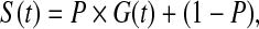
The cure-mixture model (Farewell, 1982; Yamaguchi, 1992; Peng and others, 1998) assumes the marginal survival function

(3.1)

where P is the probability of membership in the non-cured fraction and G(t) is the survival function given membership in the non-cured fraction. Farewell modeled P using logistic regression and G using Weibull PH regression (Farewell, 1982). This is a latent-class model because cure status is indeterminate for some subjects: Those who experience an event are known to be in the non-cured fraction, whereas those who are censored may belong to either fraction.

The naïve application to cure-mixture data of ordinary survival models such as Cox regression confounds estimates of hazard and predictor effects with cure probability. Thus, the survival model may identify effects that are properly associated with class membership rather than time to event (Sy and Taylor, 2000; Price and Manatunga, 2001). The bias can be revealed by examining how the marginal or unconditional hazard h_u(t) relates to the hazard h_c(t) conditional on membership in the non-cured class. The unconditional hazard for a subject drawn from the mixture is

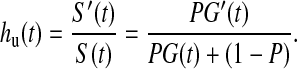By comparison, the hazard for a subject known to be in the non-cured fraction is h_c(t)=G^′(t)/G(t). Thus, the relationship between the conditional and unconditional hazards is given by h_u(t)=w(t)h_c(t), where

(3.2)

which, for proper G(t), equals 1 for all t only if P=1. We interpret w(t) as the conditional probability that a subject belongs to the non-cured fraction given survival to time t.

Assuming a randomized trial with active and control arms, we define the conditional hazard for the non-cured fraction as h_c1(t) on active and h_c0(t) on control. The conditional HR for treatment, assuming PH, is then

By comparison, the unconditional HR is

(3.3)

where w₁(t) and w₀(t) are the values of w(t) for treatment and control, respectively.

4. Definition and properties

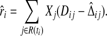
Let X_j=(X_j1,…,X_jp)^′ be the vector of predictors for individual j and X_(i) be the predictor vector for the individual who experiences the ith ordered failure at time t_i. The Schoenfeld residual for subject i is the difference between the observed predictor value and the expected predictor value (averaged across the risk set R(t_i) at t_i), given that exactly one subject fails at t_i:

(4.1)

where is the vector of estimated coefficients in a standard PH model.

Now assume the cure model (3.1) where for subject j the probability of cure is , the survival function given not cured is G_j(t), and the hazard given not cured is 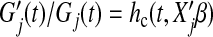, where β and ϕ are vectors of coefficients. We assume that X_j contains all predictors that affect either cure or survival.

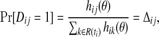
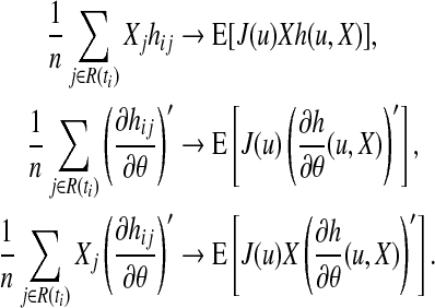
Our residual adapts the Schoenfeld residual to the cure model by using the unconditional hazard h_u as the weight in calculating the average predictor vector. Setting

and D_ij to be the indicator that subject j died at the ith ordered event time t_i, we define

(4.2)

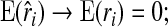
Replacing coefficients with their maximum likelihood estimates (MLEs) in (4.2), β by and ϕ by , and setting

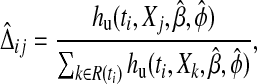our residual is

(4.3)

It is equivalent to Schoenfeld's when the cure probability is assumed to be 0 and the survival model is of PH form.

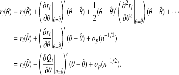
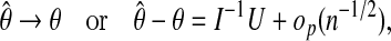
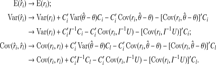
In Appendix, we demonstrate that if the model is correctly specified using m coefficient parameters, then as the residuals have the following properties:

(4.4)

(4.5)

(4.6)

where C_i is an m×p matrix of constants (see Appendix for details), I the Fisher information for (β, ϕ), and U the score function.

5. Simulation

We used simulation to examine the small-sample properties of the residuals and to explore patterns arising in the residuals when the assumed model is incorrect. An exhaustive study of possible misspecifications was impracticable. Instead, we focused on examples where data were generated from one commonly used survival distribution but fitted by another, and on the one case of a time-varying treatment effect, implemented by allowing the shape of the survival curve to differ between drug and placebo groups (Carroll, 2003. We conducted all simulations in Stata Version 11 (Stata Corporation; College Station, TX), using the maximum-likelihood utility to estimate cure models.

All simulations incorporated non-zero treatment effects on both survival and cure. We assumed a logistic cure component, with a placebo non-cure fraction of 80% and an OR for the drug effect of 0.7. Wesimulated from four different models for survival given not cured: the Weibull, Gompertz, log-normal, and log-logistic (see Table1). For each model, we chose parameters so that total censoring in the non-cured class was roughly 10% at day 220; parameter values appear in Figure2. To simulate the mean residual across time, we generated 2000 replicates of data sets of n=400 subjects at risk at day 0. For each simulated data set, we fitted each of the four models and calculated standardized residuals. Roughly of the events were censored, including both cured and non-cured classes. We then smoothed each replicate of the standardized residuals over event time using lowess with a bandwidth of 0.4.

Table 1.

Parametric survival models used in our simulations and analysis of the smoking data

Distribution	Survival function G(t)	Predictor model	Regression predictors	Shape parameters
Weibull		PH		p=eγ
Gompertz		PH		γ
Log-normal		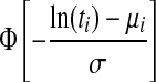AFT	μi=X′iβ	σ
Log-logistic	(1+(λit)1/p)−1	AFT		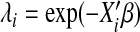p=eγ

PH, proportional hazards; AFT, accelerated failure time.

Fig. 2.

Smoothed parametric cure-model residuals for the simulated data.

Figure2 displays mean smoothed residual curves, averaged across replicates. Frames A and C represent data generated under the Gompertz and Weibull models, respectively, which incorporate predictor effects with a PH assumption. Frames B and D represent data generated under log-logistic and log-normal models, respectively, which incorporate predictor effects with an accelerated failure time (AFT) assumption. Frame E represents a model with a time-varying predictor effect, which agrees with none of the assumed models. When the generating and fitting models agree, residuals behave as the theory predicts, taking a mean near zero at all times. When the generating and fitting models disagree, the overall mean residual is zero but the mean by time deviates from zero in a curvilinear fashion.

Similar patterns can arise from misspecification of the cure class membership model. Example plots appear in supplemental materials at Biostatistics online.

6. Testing for lack of fit

Figure2 demonstrates that visual inspection of the residual plot readily reveals inadequacy of the survival model. One can also extract a formal test from the analysis of patterns like those in Figure2. An obvious candidate is a χ² test on the sum of squared standardized residuals; at least with discrete predictors, however, the χ² approximation is poor. As shown in Equations(4.4)–(4.6), although the residuals converge to zero, their asymptotic variance is complicated, making derivation of a χ² test impracticable. Grambsch and Therneau (1994) proposed testing for a time trend in the Schoenfeld residual. We suggest instead testing a polynomial fit, because the curved patterns of residuals we have observed may not be detectable with a linear trend test. Although one would expect to be able to make such a test using the χ² distribution of the likelihood ratio (LR) statistic, in fact the distribution of this statistic appears to be nonstandard. For this reason, we recommend that one refers the polynomial LR χ² to an empirical distribution generated from a parametric bootstrap.

The test proceeds as follows: First, one estimates the parametric cure model and calculates the residuals. Next, one estimates a polynomial regression of the residuals against t, t², and t³, calculating the LR test of this model against an intercept-only model. To calculate the null distribution for this statistic, one generates M replicates (we recommend M=400) under the cure model assuming the estimated parameters from the original data, restricting the datasets to have the same number of events as the original data. One then calculates the residuals, the polynomial fit, and the LR fit statistic for each of the M simulated data sets. This parametric bootstrap distribution of the LR statistic serves as the null distribution for the LR statistic from the original data.

In a second set of simulations, we generated data using selected parametric cure models described in Table1. We then fitted all four parametric models to each data set, using sample sizes of n=500, 750, and 1000, with 200 replicates of each. For each fitted model, we calculated the LR fit statistic and null distribution (with M=400) as described above. The LR statistic was deemed significant at level α if it fell above the 100(1−α) centile of the null distribution.

Figure3 shows the power of the test as a function of sample size for selected combinations of fitted and true models. For each model, the type I error rate was roughly 5% regardless of the sample size. Power for mismatched models varied widely. Figure3 shows some of the combinations corresponding to larger deviations from zero in Figure2. Combinations leading to smaller deviations were less powerful.

Fig. 3.

Power for the parametric bootstrap test of fit.

7. Application to smoking data

We applied the method to the data of Figure1, assuming a logistic model for cure and a range of parametric models for survival given not cured. Figure4 shows the resulting residual plots. The best model was the Weibull, where the non-cure rate for placebo subjects was estimated to be 73% with a drug effect OR of 0.69 (95% CI 0.46–1.04). The estimated HR for drug was 0.56 (95% CI 0.41–0.78), compared with the HR=0.69 obtained from the Cox model without cure.

Fig. 4.

Smoothed pseudo-residuals from various cure-model fits to the bupropion clinical trial data.

Our test gave p=0.49 for the Weibull model, p=0.27 for the Gompertz, p=0.18 for the log-logistic, and p=0.25 for the log-normal. Thus, although Weibull is the best both on the basis of appearance and p value, none of the models fits significantly badly. Schoenfeld residuals revealed a time trend, indicating a violation of the PH assumption with the treatment effect HR changing over time. Our Weibull cure-mixture residuals suggest the PH assumption is reasonable within the context of a cure model.

8. Discussion

We have developed a Schoenfeld-like pseudo-residual to assess the fit of a parametric cure-mixture model. The Schoenfeld residual compares the predictor of the subject who fails at the ith failure event to its expectation, conditional on the risk set and assuming PH. Our residual differs in using the full estimated hazard to compute the conditional expectation of the predictor. The weights thus reflect the probability of membership in the non-cured class, including estimates of any parameters of the cure component of the model.

Like the original Schoenfeld residual, the plot of the smoothed cure-mixture pseudo-residual vs. event time describes a horizontal line at 0 when the model fits well. When the fit is poor, the smoothed residuals display a possibly nonlinear trend across time. One can evaluate the fit numerically with a parametric bootstrap test of a polynomial model for the residual.

A limitation of the procedure is its lack of specificity. In some cases, several models may fit equally well; the log-normal and log-logistic, for example, commonly yield similar residual patterns. The analysis may be of most value when there is some discrepancy between the inferences or predictions obtained under several models; in such cases one can use the diagnostic to identify the best-fitting model.

The residual is sensitive to departures from either component of the cure model. Our sense is that both parts of the model should include as many predictors as are available. We expect that in most situations using all available predictors will give an acceptably good fit for the cure portion of the model, particularly so when the predictors are categorical. As our simulations show, including the correct predictors is not sufficient to create a good fit for the model of survival given not cured; the residual will readily detect misspecification of the hazard function.

Supplementary material

Supplementary material is available at http://biostatistics.oxfordjournals.org.

Funding

The National Cancer Institute supported the research of Drs Heitjan and Wileyto under USPHS grant R01 CA 116723 (Heitjan), and NCI P50 CA143187 (Lerman).

Appendix: Asymptotic properties of the pseudo-residuals

We first simplify the notation, defining θ=(β,ϕ), h_ij(θ)=h_u(t_i, X_j,θ), and . That is,

If the model is correctly specified, then the hazard at time t_i for a subject with predictor X_j is h_ij(θ), and

so that the vector of D_ij values follows a multinomial distribution with parameter vector equal to the vector of Δ_ij values, for j∈R(t_i). Therefore,

(A.1)

and

(A.2)

Moreover consider two time points t_i and t_l (i<l), and note that r_i is defined conditionally on R(t_i) and r_l conditionally on R(t_l). Let D_i denote the vector of D_ij. Then

This is because given the event that occurred at time t_i, r_i is a constant vector c_p×1, and because the identity of the subject who experienced an event at t_l is unrelated to the identity of the subject who experienced an event at t_i.

We now expand r_i in θ about the MLE :

That is,

(A.3)

Note that at any given time u=t_i

(A.4)

As noted in Oakes (1977), the expression

(A.5)

where J_j(u)=0 or 1 as j∉ or j∈R(u). This has the form of a sample mean over the n subjects in the study. So under some regularity conditions (A5) will converge, as , to the expectation E[J(u)h(u,X)]. The other expressions in (A4) converge to their expectations as well:

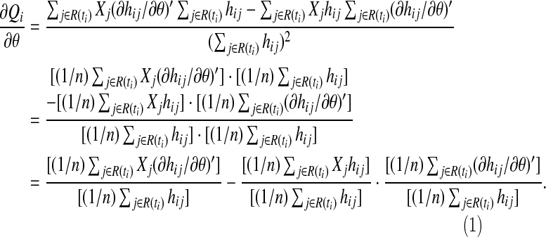
Therefore, (∂Q_i/∂θ)(θ) converges to

(A.6)

Moreover, the model is parametric and thus the MLE has the standard property (Van der Vaart, 1998):

(A.7)

where I is the Fisher information and U is the score function.

Substituting (A6) and (A7) into (A3), we have

This completes the proof.

References

- Carroll K. J. On the use and utility of the Weibull model in the analysis of survival data. Controlled Clinical Trials. 2003;24:682–701. doi: 10.1016/s0197-2456(03)00072-2. [DOI] [PubMed] [Google Scholar]
- Farewell V. T. The use of mixture-models for the analysis of survival-data with long-term survivors. Biometrics. 1982;38:1041–1046. [PubMed] [Google Scholar]
- Grambsch P. M., Therneau T. M. Proportional hazards tests and diagnostics based on weighted residuals. Biometrika. 1994;81:515–526. [Google Scholar]
- Lambert P. C., Thompson J. R., Weston C. L., Dickman P. W. Estimating and modeling the cure fraction in population-based cancer survival analysis. Biostatistics. 2007;8:576–594. doi: 10.1093/biostatistics/kxl030. [DOI] [PubMed] [Google Scholar]
- Li Y., Heitjan D. F. A note on the complementary mixture Pareto II distribution. Communications in Statistics-Theory and Methods. (in press) [Google Scholar]
- Li C. S., Taylor J. M. G., Sy J. P. Identifiability of cure models. Statistics & Probability Letters. 2001;54:389–395. [Google Scholar]
- Li Y., Wileyto E. P., Heitjan D. F. Modeling smoking cessation data with alternating states and a cure fraction using frailty models. Statistics in Medicine. 2010;29:627–638. doi: 10.1002/sim.3825. [DOI] [PMC free article] [PubMed] [Google Scholar]
- Oakes D. The asymptotic information in censored survival data. Biometrika. 1977;64:441–448. [Google Scholar]
- Peng Y. W., Dear K. B. G., Denham J. W. A generalized F mixture model for cure rate estimation. Statistics in Medicine. 1998;17:813–830. doi: 10.1002/(sici)1097-0258(19980430)17:8<813::aid-sim775>3.0.co;2-#. [DOI] [PubMed] [Google Scholar]
- Price D. L., Manatunga A. K. Modelling survival data with a cured fraction using frailty models. Statistics in Medicine. 2001;20:1515–1527. doi: 10.1002/sim.687. [DOI] [PubMed] [Google Scholar]
- Schoenfeld D. Partial residuals for the proportional hazards regression-model. Biometrika. 1982;69:239–241. [Google Scholar]
- Sy J. P., Taylor J. M. G. Estimation in a Cox proportional hazards cure model. Biometrics. 2000;56:227–236. doi: 10.1111/j.0006-341x.2000.00227.x. [DOI] [PubMed] [Google Scholar]
- Van der Vaart A. W. Asymptotic Statistics. New York, NY: Cambridge University Press; 1998. [Google Scholar]
- Weston C. L., Douglas C., Craft A. W., Lewis I. K., Machin D. Establishing long-term survival and cure in young patients with Ewing's sarcoma. British Journal of Cancer. 2004;91:225–232. doi: 10.1038/sj.bjc.6601955. [DOI] [PMC free article] [PubMed] [Google Scholar]
- Wileyto E. P., Patterson F., Niaura R., Epstein L. H., Brown R. A., Audrain-McGovern J., Hawk L. W., Lerman C. Recurrent event analysis of lapse and recovery in a smoking cessation clinical trial using bupropion. Nicotine & Tobacco Research. 2005;7:257–268. doi: 10.1080/14622200500055673. [DOI] [PubMed] [Google Scholar]
- Yamaguchi K. Accelerated failure-time regression-models with a regression-model of surviving fraction—an application to the analysis of permanent employment in Japan. Journal of the American Statistical Association. 1992;87:284–292. [Google Scholar]
Associated Data
This section collects any data citations, data availability statements, or supplementary materials included in this article.