Multicategory reclassification statistics for assessing improvements in diagnostic accuracy

Abstract

In this paper, we extend the definitions of the net reclassification improvement (NRI) and the integrated discrimination improvement (IDI) in the context of multicategory classification. Both measures were proposed in Pencina and others (2008. Evaluating the added predictive ability of a new marker: from area under the receiver operating characteristic (ROC) curve to reclassification and beyond. Statistics in Medicine 27, 157–172) as numeric characterizations of accuracy improvement for binary diagnostic tests and were shown to have certain advantage over analyses based on ROC curves or other regression approaches. Estimation and inference procedures for the multiclass NRI and IDI are provided in this paper along with necessary asymptotic distributional results. Simulations are conducted to study the finite-sample properties of the proposed estimators. Two medical examples are considered to illustrate our methodology.

1. Introduction

Diagnostic and classification tasks are encountered in medical practice where we need to accurately differentiate the disease-present and the disease-absent status of a patient. Sometimes the classification may involve more than two categories which need to be treated separately. For example, one of the motivating examples of this paper is a classification for synovitis where patients from five distinct disease categories are examined, each requiring a different patient management strategy. Health-care procedures are decided based on the determination of the most likely status of the patient. Biomarkers are often used to predict the patient's disease status, drawing upon a set of well-established statistical tools for evaluating diagnostic accuracy.

Typically, in binary classification, one employs statistical methods based on the receiver operating characteristic (ROC) analysis and provides the estimated ROC graph and/or summary measures of the ROC graph such as the area under the curve (AUC) or the partial AUC (Zhou and others, 2002. Such methods vary the threshold used to classify individuals as diseased and non-diseased and then combines the resulting sensitivities and specificities across all possible thresholds. The extensions of these methods to multicategory classification have been recently proposed. Specifically, we may use the hypervolume under the multidimensional ROC manifold (HUM) as an extension of the AUC to evaluate the classification accuracy for any biomarker in a multiclass problem (Mossman, 1999. The HUM has an interpretation akin to the AUC where a large HUM value indicates a high classification accuracy. The inference procedure for the HUM has been discussed in Nakas and Yiannoutsos (2004) for ordered polychotomous responses and Li and Fine (2008) for unordered polychotomous responses. Shiu and Gatsonis (2012) provides a review of ROC-type methods for multiclass problems.

While ROC-based measures have been widely adopted, it has been argued by many authors (Pepe and others, 2004; Pencina and others, 2008 that such measures may not be good criteria to quantify improvements in diagnostic accuracy when the added value of a new predictor to an existing model is of interest. Such analyses are critically important in the development of predictive models based on biomarkers, where the added value of markers which may be expensive to obtain must be weighed against the associated financial costs. The interpretation of the AUC provides an indirect assessment of the predictive performance of a model. Thus, the gain with a new predictor may be unclear. A related issue is that the AUC measures may be relatively insensitive to the addition of predictors in certain regions of the AUC space. To address these limitations, Pencina and others (2008) proposed two novel criteria based on reclassification in order to directly quantify the extent to which a new predictor improves classification performance: the net reclassification improvement (NRI) and the integrated discrimination improvement (IDI). These measures have met with widespread success in the medical literature, with many practitioners preferring their ease of interpretation versus ROC-based measures. For additional discussion of these recent developments, we refer the reader to Pencina and others (2011, 2012).

In this paper, we extend the reclassification indices to multicategory classification problems, providing an alternative to HUM-based analyses. The multicategory definitions of the NRI and the IDI are presented in Section2.1, with their inferential procedures described in Section2.2. The use of such measures in model building is discussed in Section2.3, with an eye toward high-dimensional data structures, where the number of predictors may be much larger than the sample size. Extensive numerical studies are conducted. Simulations are reported in Section3, with two real data examples presented in Section4, including the synovitis example mentioned previously and a microarray example, where it is important to select a small number of the most important expression biomarkers for the prediction of cancer (Li and Fine, 2008; Ma and Song, 2011, among others).

2. Methods

2.1. Accuracy parameters

Consider a set of predictors Ω={X₁,…,X_p}. Suppose that we have a sample of subjects with measurements of all X_j (j=1,…,p). The goal is to use them to construct a meaningful statistical model for predicting the multicategory outcome Y which takes values from . We define the binary random variable Y _m=I(Y =m) and let the prevalence for the mth category be ρ_m=E(Y _m)=P(Y =m).

Suppose that a model is constructed based on a set of predictors Ω₁⊂Ω. Such a model can generate a probability vector …, for each subject where =1. Decision makers may assign a subject to one of the M categories according to the greatest component in the probability vector. One may quantify the accuracy of based on Ω₁ by the following multicategory correct classification probability (CCP):

(2.1)

where each CCP_m is the CCP for the mth-category. For the model , we write

(2.2)

Now suppose that more variable(s) are included and we construct a model that is based on a set of predictors . We use the nested-structure notations as they are widely discussed in the literature. We note that there are plenty of cases where the accuracy improvement occurs among non-nested models. Our proposed methods can apply with slight modification.

The newly constructed model generates another probability vector …, for each subject where . Again, decision makers may assign the subject according to the greatest value of this probability vector, and the mth-category accuracy of based on Ω₂ can be quantified by

(2.3)

The overall accuracy improvement from to may be summarized as

(2.4)

where w_m are positive weights for the mth category. When M=2, the two CCPs are usually called the sensitivity and specificity of the model-based test. The T measure thus quantifies the overall increase of the weighted sum of sensitivity and specificity. When equal weights are used for the two categories, T is simply the difference of Youden's index between the two models. We shall call (2.4) the reclassification improvement (RI) since it reflects how the accuracy changes after a reclassification.

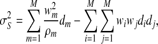
The RI measure has well-known limitations in assessing improvements in diagnostic accuracy and has not been widely adopted in practice (Pencina and others, 2008. Here, we propose to extend the NRI, which has recently been studied as an alternative to the RI for binary classification. The multicategory extension of the NRI is

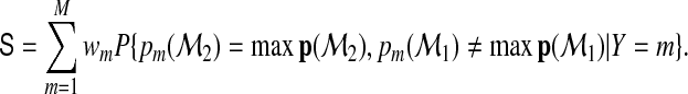(2.5)

When M=2 and , S is equivalent to the NRI given in Pencina and others (2008). We refer to S as the NRI in this article since it indicates the probability that added markers in lead to correct classification of subjects who are incorrectly classified using the smaller model . We note that, in the two-category classification, the decision can be based on whether the class probability exceeds with equal priors on the two categories.

The IDI can be generalized to multiple categories by noticing the connection between the IDI in binary classification problems and R² (Cox and Wermuth, 1992; Menard, 2000; Tjur, 2009). The interpretation and computation of R², also called a coefficient of determination, has been discussed for binary logistic regression models. Simply speaking, the value of R² is the fraction of the total variation explained by the model. For linear regression models, R² is closely related to the correlation coefficient and the ANOVA F-test, while for binary regression, it is closely connected to the probabilities of correct classification.

Let be an M-dimensional vector with

(2.6)

The second equality follows because . It has been shown in Pepe and others (2008) that the increase in R² for binary classification (M=2) from model to model is equivalent to the IDI in Pencina and others (2008). A natural adaptation of the R² definition of the IDI to the multicategory set-up is

(2.7)

We refer to (2.7) as the IDI in this paper, similarly to the binary case. The multicategory IDI (2.7) reduces to that in Pencina and others (2008) when M=2 and equal weights are used.

The choice of weights in the definitions of the NRI and the IDI may depend on the goal and design of the study. When aiming for the overall test accuracy to differentiate multiple classes, it is natural to weigh all categories equally; on the other hand, as pointed out in Pencina and others (2011), sometimes it is useful to reward some categories with higher weights when savings associated with correct classification of such categories outweigh other categories. When cost-efficiency information is available, we can incorporate them easily in the inference for the weighted NRI and IDI. There are also other practical considerations that invoke unequal weights and one can run a Bayesian prior elicitation procedure to construct reasonable weights (Li and Fine, 2010).

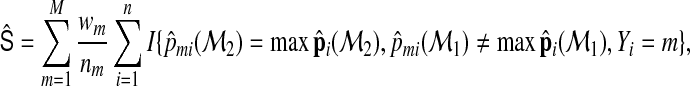
2.2. Estimation theory

Suppose we obtain a sample {X_i1,…,X_ip,Y _i:i=1,…,n}. We denote the class sample size for the mth category. We assume that and n_m/n→ρ_m>0 for all m. One may fit the candidate models and from the preceding subsection using one's method of choice. The main requirement is that the method provide estimated probability assessment vectors for each model. Using the fitted models, one may then estimate the two reclassification accuracy measures RI and NRI by

(2.8)

and

(2.9)

where is the estimated membership probability for the ith subject based on the jth model. In practice, they can be obtained from fitting a multinomial logistic regression model to the data and then outputting the predicted probabilities from the fitted model. We note that when the models are consistently estimated, is consistent to and therefore, by the law of large numbers, and are consistent to T and S, respectively. Furthermore, by using the central limit theorem, we can show that , where

(2.10)

with , , , and , where

(2.11)

with . We note that the terms following in and are not independent. We obtain independent sums only after changing the order of summation and then are able to apply the central limit theorem. In practice, all the components involved in the variance expressions can be consistently estimated by plugging in the sample version of the probabilities.

The multicategory IDI can be estimated by using the following formula:

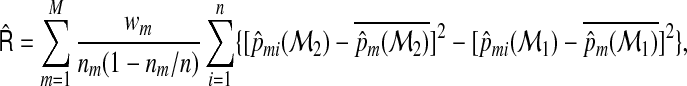(2.12)

where .

We can also show that (2.12) is consistent to R for a large n by noting that, for a large sample, is consistent to , and the average squared distance to the mean 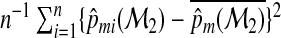is consistent to . The consistency then follows from the law of large numbers. As with RI and NRI, one may further show that ,where

(2.13)

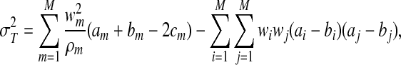
and . All the moments involved in the variance expression can be readily estimated by using empirical moment estimators. The variance can then be estimated by the plug-in method.

The above parameter estimation and variance estimation formula are implemented in the software R and the code is downloadable at http://www.stat.nus.edu.sg/~stalj. Although the variance formula (2.11) and (2.13) look complicated in the above presentation, our experiences with simulation and real data analysis suggest that they can be evaluated instantly following the point estimation by using our code. These formula allow inferences to be carried out much faster than a resampling-based approach. An advantage of the resampling method is that the sampling variability in the estimation of the probability vector may be formally accounted for in the inference.

2.3. Model-building procedure

For biomedical data with ever-growing dimensionality and complexity, we often face the challenge p≫n and cannot afford using all p markers for the construction of a feasible prediction model. We now propose a procedure to select important predictors for regression analysis with multicategory response. Specifically, we adopt a forward selection algorithm by using the NRI and the IDI as the selection criteria. The model-building algorithms are similar for the two criteria. We thus choose to present the detailed procedure for the NRI only.

We start with a null model. At the first step, we fit regression models with a single covariate for all X_j j=1,…,p and evaluate the NRI for each X_j. The variable that gives the highest NRI value is chosen at this stage. At the second step, we fit regression models with the previously selected predictor and another predictor in the remaining set. We evaluate the NRI again for each model and then select the best model according to the highest NRI. The selection procedure proceeds until a stopping rule is satisfied.

We consider two stopping rules in this paper. Rule I stops the model-building procedure when a pre-specified number of predictors or pre-specified proportion of all predictors is achieved. Rule II stops the model-building procedure when a pre-specified full-model accuracy is achieved, for example, 90% of the overall CCP. When resources are limited and only a fixed number of markers can be fully investigated in a study, we may consider Rule I and retain a relatively parsimonious model; on the other hand, when there is sufficient support that allows us to examine as many markers as possible, we may target a very high accuracy and choose Rule II. As demonstrated in the microarray analysis in Section4.2, it may be possible to achieve 100% accuracy in some applications. Simulation studies included in supplementary material available at Biostatistics online find satisfactory performance of this forward selection method.

3. Simulation analysis of estimation consistency

In this section, we used simulation studies to examine the performance of our proposed estimators and for the NRI and the IDI, respectively. We consider six different scenarios.

Case 1. We first consider a three-category response with the following multinomial logistic structure:

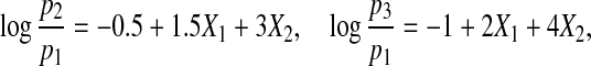where p_j=P(Y =j) for j=1,2,3. We generate (X₁,X₂) from a multivariate normal distribution with mean (1,1) and covariance matrix Σ=(σ_i,j)_1≤i,j≤2. We let σ₁₁=σ₂₂=1, and σ₁₂=σ₂₁=0 and let , .

Case 2. The same as Case 1 except that we let σ₁₂=σ₂₁=0.2.

Case 3. Next we increase the number of covariates and consider the following three-category response model:

We generate (X₁,X₂,…,X₅) from a multivariate normal distribution with mean (1,1,1,1,1) and covariance matrix Σ=(σ_i,j)_1≤i,j≤5. We set Σ=diag{1,1,1,1,1} and let , .

Case 4. The same as Case 3 except that we let σ_ij=0.1,i≠j. This imposes a compound symmetry dependence structure for the covariates.

Case 5. Next we consider a five-category response by using the following multinomial logistic structure:

We generate (X₁,X₂,X₃) from a multivariate normal distribution with mean (1,1,1) and covariance matrix Σ=diag(1,1,1), .

Case 6. The same as Case 5 except that we set σ₁₂=σ₂₁=σ₂₃=σ₃₂=0.1.

For each case, we simulated 1000 data sets and carried out the estimation procedures for the NRI and the IDI introduced in the previous section. The numerical results are summarized in Table1. Eyeballing Table1, we notice that both and perform very well in estimating S and R, respectively, in all cases. The variance formula for the NRI and the IDI also provide very close approximation to the sampling variability of the estimators. The coverage rates are close to 95% and improve as the sample size increases. We note that in some cases the coverage of the IDI is slightly lower than the nominal level. The undercoverage issue may be caused by the fact that we do not account for the sampling variability of the regression estimation. Another factor is that normal approximation is not appropriate when the IDI is close to zero. After acknowledging the estimation uncertainty, Kerr and others (2011) derived an approximate χ² distribution under the null for the two-category classification. Another alternative approach is to consider the bootstrap.

Table 1.

Performance of and over 1000 simulations

	S	Avg.SDS			CRS	R	Avg.SDR			CRR
Case 1
n=150	0.263	0.067	0.271	0.055	0.977	0.263	0.053	0.279	0.052	0.925
n=300	0.263	0.047	0.269	0.040	0.973	0.263	0.036	0.272	0.036	0.937
Case 2
n=150	0.238	0.059	0.246	0.057	0.955	0.252	0.049	0.262	0.050	0.935
n=300	0.238	0.042	0.246	0.041	0.952	0.252	0.034	0.258	0.034	0.951
Case 3
n=150	0.282	0.094	0.322	0.076	0.977	0.319	0.088	0.385	0.085	0.938
n=300	0.282	0.062	0.298	0.051	0.977	0.319	0.054	0.346	0.052	0.946
Case 4
n=150	0.302	0.083	0.317	0.071	0.976	0.334	0.076	0.384	0.077	0.930
n=300	0.302	0.056	0.305	0.048	0.969	0.334	0.049	0.356	0.049	0.944
Case 5
n=150	0.226	0.057	0.251	0.046	0.975	0.178	0.039	0.203	0.038	0.922
n=300	0.226	0.039	0.237	0.032	0.975	0.178	0.025	0.186	0.024	0.942
Case 6
n=150	0.223	0.053	0.249	0.046	0.953	0.183	0.036	0.206	0.036	0.900
n=300	0.223	0.037	0.238	0.033	0.957	0.183	0.024	0.194	0.024	0.939

S and R are the true value of NRI and IDI computed using Monte Carlo; avg.SD_S and avg.SD_R are mean of estimated SEs of and computed based on (2.11) and (2.13) over 1000 simulations; and are the mean and standard deviation of the estimated NRI over 1000 simulations; and are the mean and standard deviation of the estimated IDI over 1000 simulations; CR_S=(number of simulations the true NRI falling into the interval CR_R=(number of times the simulations the true IDI falling into the interval .

4. Examples

We first consider a medical study with five categories to illustrate the applications of the NRI and the IDI for a practical assessment of accuracy improvement. A second analysis utilizes data from a genetic study to demonstrate how the NRI and the IDI can be used for variable selection in high-dimensional data analysis. Since the HUM has previously been employed for model selection in multicategory set-ups, we explicitly compare the HUM to the new measures, with a focus on interpretation and model selection issues.

4.1. Tissue biomarkers of synovitis

Synovitis is the inflammation of the synovial membrane and may occur in association with arthritis as well as lupus, gout, and other conditions. Krenn and others (2006) and Slansky and others (2010) described a scoring approach to evaluate the grading of the histological severity of synovitis. In their data set, the primary classification outcome involved five different categories: normal healthy control; Post-traumatic Arthropathy (PtA); Osteoarthritis (OA); Psoriatic Arthritis (PsA); Rheumatoid Arthritis (RA). The sample included a total of 583 synovial tissue specimens taken from 33 normal, 29 PtA, 221 OA, 42 PsA, and 341 RA subjects, respectively. Details of the sample collection procedures were included in earlier publications (Krenn and others, 2006; Slansky and others, 2010).

Three biological measurements are commonly used to predict the patient disease status: the lining thickness, the inflammatory infiltrates, and the stromal density. Each of the three biomarker components was graded on a scale from zero to three in the sample. The accuracy of the three biomarkers for pairwise binary classification and five-category classification were reported in Krenn and others (2006) and Slansky and others (2010). We use our proposed approach to evaluate the relative improvement for increasing the marker numbers in a statistical model. For the ease of presentation and comparison, we denoted the lining thickness as X₁, the stromal density as X₂, and the inflammatory infiltrates as X₃ in this paper. We first quantified the diagnostic accuracy for each component and then combined them with the multinomial logistic regression to further improve the diagnostic accuracy.

The estimated NRI and IDI are reported in Table2. The models with a single covariate are not nested and cannot be compared using the NRI and the IDI. Instead, we report their CCP in the NRI column and their R² values in the IDI column. The second marker X₂ has the highest CCP and IDI and is considered as the most accurate one. The CCP indicates that over 65% of the sample were correctly classified by X₂, while the IDI indicates that approximately 12% of the overall variability of the five-category response may be attributed to X₁. The other two markers have relatively inferior performance, with X₃ being the next most accurate marker and followed by X₁. This finding is consistent to the previous observations in Slansky and others (2010) using ROC-based diagnostic accuracy measures, with the estimated HUMs for X₁, X₂, and X₃ being 0.0005, 0.0140, and 0.0075, respectively.

Table 2.

Estimated NRI and IDI and SEs for three synovitis biomarkers: lining thickness (X₁), stromal density (X₂), and inflammatory infiltrates (X₃)

Model(s)	NRI (SE)	IDI (SE)
X1	0.5746 (0.0081)	0.0555 (0.0168)
X2	0.6518 (0.0078)	0.1174 (0.0304)
X3	0.5866 (0.0085)	0.0751 (0.0180)
X1+X2 versus X2	0.0030 (0.0017)	0.0102 (0.0021)
X3+X2 versus X2	0.0385 (0.0056)	0.0302 (0.0024)
X1+X2+X3 versus X2+X3	0.0013 (0.0009)	0.0062 (0.0015)

For models with only one marker, NRI is the overall model CCP and IDI is the model R². For others, NRI is the NRI value and IDI is the increase in IDI for the two nested models (X₃).

It is of interest to combine X₂ with other marker(s) to improve the overall diagnostic accuracy. NRI results suggest that a two-marker model combining X₂ with X₃ (NRI=0.0385) may result in a larger improvement in classification accuracy than with X₁ (NRI=0.0030). The NRI values indicate that the improvement on a model-based net reclassification rate due to including X₃ is more than 10 times of that due to including X₁. We note that marker X₃ has the second highest CCP 0.5866 in the one-marker model. The standard errors (SEs) in the brackets allow us to construct the Wald-type tests. In this case, it seems that the NRI improvement for the addition of X₃ is highly significant, whereas that for adding X₁ is not.

On the other hand, IDI results show a similar preference for X₃. The IDI improvement for including X₃ (IDI=0.0302) is three times of that for including X₁ (IDI=0.0102), indicating that the addition of X₃ could explain much more variability in the response. Using the SEs, we carried out the Wald tests and found that both IDI increases were significantly different from zero.

In practice, the final model including three markers is always considered as it yields the highest CCP and IDI. Moving from model {X₂+X₃} to model {X₁+X₂+X₃}, the NRI is not significant (Wald test |0.0013/0.0009|<1.96), while the IDI is highly significant (Wald test |0.0062/0.0015|>1.96). These divergent results require careful interpretation because the two measures need to be construed from different perspectives. Adding X₁ in the last stage may not significantly improve the number of correct classifications from the previous model. However, it may still contribute a significant amount of information and help explain the overall variability of the response.

The results in Table2 are interesting to investigators as how the model accuracy evolved with the added complexity was clearly presented and the relative contribution of each marker to the overall classification was fully demonstrated. The earlier findings in Slansky and others (2010) reported the accuracy for individual markers (in the absence of information from other markers) but failed to inform the added accuracy of new markers in the presence of other already selected marker(s).

4.2. Leukemia classification

We next consider data from leukemia patients used in Golub and others (1999). The data are from a study of gene expression in three types of acute leukemias, acute lymphoblastic leukemia arising from T-cells (ALL T-cell), ALL arising from B-cells (ALL B-cell), and acute myeloid leukemia (AML). The data set contains 8 ALL T-cell samples, 19 ALL B-cell samples, and 11 AML samples. Each sample contains 7912 gene expression values obtained from Affymetrix high-density oligonucleotide microarrays. Our data set is downloaded from http://www.broad.mit.edu/cgi-bin/cancer/datasets.cgi.

We consider evaluating the accuracy of the biomarkers for their ability to differentiate the three classes. The single gene that gives the highest CCP is the 1184th gene in the data file, with a CCP value 0.8421. We then use the methods in this paper to select a second gene which maximizes the accuracy improvement. By using the NRI, the best gene is the 2216th gene with an NRI value 0.2145 and SE 0.0678 (P-value 0.0015). Adding the 2216th gene could correctly identify about 20% of the observations that cannot be correctly classified by using only the 1184th gene. In fact, with these two genes, we reach a 100% overall CCP value and obtain a perfect classification for the three categories. The empirical distribution of all NRI values is shown in the left panel of Figure1. The mode of the distribution is around 0.05, indicating a 5% improvement over the existing marker.

Fig. 1.

Empirical distribution of NRI and IDI values for all gene expressions of the Leukemia example.

We have used the IDI for this data set and obtained the same results. At the first step, the 1184th gene was selected with the highest IDI 0.6364, while at the second step the 2216th genes was added for providing the most IDI increase 0.3906 (SE 0.0696). No further improvement in the IDI can be attained with additional genes. The empirical distribution of all IDI values is shown in the right panel of Figure1. The distribution for the IDI is more skewed than that for the NRI.

Many authors examined this data set using various classification methods such as machine learning (Golub and others, 1999; Furey and others, 2000; Guyon and others, 2002, threshold circuits (Albrecht and others, 2003), rigid regression (Li and Yang, 2005), and stochastic search (Albrecht, 2007). The numbers of gene expression levels used in their studies were all greater than 2. The most similar previous results may be found in Li and Yang (2005) and Albrecht (2007), where only three genes were needed to achieve the same accuracy. Our findings based on NRI and IDI selection appear to be a further improvement from the existing analyses.

We may further use this example to compare across different methods. Besides the NRI and the IDI, a common ROC-based measure for multicategory classification is the HUM (Li and Fine, 2008). The results of using the HUM are the same as those obtained as using the NRI and the IDI: selecting the 1184th gene with the highest HUM value 0.8116 at the first step, and selecting the 2216th gene with the highest HUM improvement at the second step. This results in the same two genes being selected (in the same order) to give a 100% HUM in the final model. However, in general the agreement between the three approaches varies because they focus on different aspects of the model accuracy. The sample correlation coefficient between the NRI and the IDI values at the second selection step was 0.747. The scatter plot of the IDI versus the NRI is given in the upper left panel of Figure2, displaying an increasing association. The correlation between HUM and NRI was only 0.627 and the scatter plot of HUM versus NRI is given in the upper right panel of Figure2. The correlation between HUM and IDI was 0.859, showing a strong dependence pattern in the lower panel of Figure2. All correlations are positive and strong, exceeding 0.60, with the association between IDI and HUM suggesting that, at least in this example these measures provide the most similar assessment of improvements in leukemia classification accuracy.

Fig. 2.

Scatterplots of IDI versus NRI, NRI versus HUM and IDI versus HUM for gene expressions in the leukemia example.

5. Discussion

While in the numerical studies, multinomial logistic regression was employed for constructing the probability assessment, in practice, any procedure providing such assessments could be used. The simplicity of the logistic analysis is appealing and is theoretically supported by the recent work of Delaigle and Hall (2012), who established that optimal classification can be achieved with a linear method for Gaussian data. Considering that normal distribution is perhaps the most prevalent for discrimination and classification (Pencina and others, 2012), the linear combination approach, thus, may provide satisfactory performance in a wide range of real data applications in the biomedical sciences.

Besides the multinomial logistic regression model, we have also experimented with the support vector machine as an alternative classifier and found its performance to be comparable with that of multinomial logistic regression in simulations. Code implementing such analyses is available at the first author's website mentioned earlier. An advantage of logistic regression beyond classification is that the coefficients may be easily interpreted and yield insight into the markers’ effects on the response. Another observation is that the sampling behavior of NRI and IDI estimates seems less stable for the support vector machine when the sample size is small.

It is important to note that the evaluation of the NRI and the IDI must be based on correctly calibrated models, especially when the old and new models are not nested. In numerical studies, we have observed that the probability assessments from incorrectly calibrated non-nested models could be surprisingly different and that calculations based on such quantities may not yield reasonable results. That is, spurious improvements in the NRI and the IDI may be achieved when either one or both of the models fit poorly. In such scenarios, the improvements are confounded by the lack of fit of the models, potentially leading to incorrect conclusions about the predictive values of added biomarkers. In general, careful consideration of model calibration, including goodness-of-fit diagnostics, is needed to ensure adequate model fit prior to model comparisons based on the NRI and the IDI.

Supplementary material

Supplementary material is available at http://biostatistics.oxfordjournals.org.

Funding

This work was supported by grants from Academic Research Funding R-155-000-130-112 and National Medical Research Council NMRC/CBRG/0014/2012.

References

- Albrecht A. Stochastic local search for the feature set problem, with application to microarray data. Applied Mathematics and Computation. 2007;183:1148–1164. [Google Scholar]
- Albrecht A., Vinterbo S. A., Ohno-Machado L. An epicurean learning approach to gene-expression data classification. Artificial Intelligence in Medicine. 2003;97:245–271. doi: 10.1016/s0933-3657(03)00036-8. [DOI] [PubMed] [Google Scholar]
- Cox D. R., Wermuth N. A comment on the coefficient of determination for binary response. The American Statisticians. 1992;46:1–4. [Google Scholar]
- Delaigle A., Hall P. Achieving near-perfect classification for functional data. Journal of the Royal Statistical Society: Series B. 2012;74:267–286. [Google Scholar]
- Furey T. S., Cristianini N., Duffy N., Bednarski D. W., Schummer M., Haussler D. Support vector machine classification and validation of cancer tissue samples using microarray expression data. Bioinformatics. 2000;16:906–914. doi: 10.1093/bioinformatics/16.10.906. [DOI] [PubMed] [Google Scholar]
- Golub T. R., Slonim D. K., Tamayo P., Huard C., Gaasenbeek M., Mesirov J. P., Coller H., Loh M. L., Downing J. R., Caligiuri M. A. Molecular classification of cancer: class discovery and class prediction by gene expression monitoring. Science. 1999;286:531–537. doi: 10.1126/science.286.5439.531. and others. [DOI] [PubMed] [Google Scholar]
- Guyon I., Weston J., Barnhill S., Vapnik V. Gene selection for cancer classification using support vector machines. Machine Learning. 2002;46:389–422. [Google Scholar]
- Kerr K. F., McClelland R. L., Brown E. R., Lumley T. Evaluating the incremental value of new biomarkers with integrated discrimination improvement. American Journal of Epidemiology. 2011;174:364–374. doi: 10.1093/aje/kwr086. [DOI] [PMC free article] [PubMed] [Google Scholar]
- Krenn V., Morawietz L., Burmester G. R., Kinne R. W., Mueller-Ladner U., Muller B., Haupl T. Synovitis score: discrimination between chronic low-grade and high-grade synovitis. Histopathology. 2006;49:358–364. doi: 10.1111/j.1365-2559.2006.02508.x. [DOI] [PubMed] [Google Scholar]
- Li J., Fine J. P. ROC analysis for multiple classes and multiple categories and its application in microarray study. Biostatistics. 2008;9:566–576. doi: 10.1093/biostatistics/kxm050. [DOI] [PubMed] [Google Scholar]
- Li J., Fine J. P. Weighted area under the receiver operating characteristic curve and its application to gene selection. Applied Statistics. 2010;59:673–692. doi: 10.1111/j.1467-9876.2010.00713.x. [DOI] [PMC free article] [PubMed] [Google Scholar]
- Li F., Yang Y. Analysis of recursive gene selection approaches from microarray data. Bioinformatics. 2005;21:3741–3747. doi: 10.1093/bioinformatics/bti618. [DOI] [PubMed] [Google Scholar]
- Ma S., Song X. Ranking prognosis markers in cancer genomic studies. Briefings in Bioinformatics. 2011;12:33–40. doi: 10.1093/bib/bbq069. [DOI] [PMC free article] [PubMed] [Google Scholar]
- Menard S. Coefficients of determination for multiple logistic regression analysis. The American Statisticians. 2000;54:17–24. [Google Scholar]
- Mossman D. Three-way ROCs. Medical Decision Making. 1999;19:78–89. doi: 10.1177/0272989X9901900110. [DOI] [PubMed] [Google Scholar]
- Nakas C. T., Yiannoutsos C. T. Ordered multiple-class ROC analysis with continuous measurements. Statistics in Medicine. 2004;23:3437–3449. doi: 10.1002/sim.1917. [DOI] [PubMed] [Google Scholar]
- Pencina M. J., D'Agostino R. B., Sr, D'Agostino R. B., Jr, Vasan R. S. Evaluating the added predictive ability of a new marker: from area under the ROC curve to reclassification and beyond. Statistics in Medicine. 2008;27:157–172. doi: 10.1002/sim.2929. [DOI] [PubMed] [Google Scholar]
- Pencina M. J., D'Agostino R. B., Sr., Demler O. V. Novel metrics for evaluating improvement in discrimination: net reclassification and integrated discrimination improvements for normal variables and nested models. Statistics in Medicine. 2012;31:101–113. doi: 10.1002/sim.4348. [DOI] [PMC free article] [PubMed] [Google Scholar]
- Pencina M. J., D'Agostino R. B., Sr, Steyerberg E. W. Extensions of net reclassification improvement calculations to measure usefulness of new biomarkers. Statistics in Medicine. 2011;30:11–21. doi: 10.1002/sim.4085. [DOI] [PMC free article] [PubMed] [Google Scholar]
- Pepe M. S., Feng Z., Gu J. W. Comments on ‘Evaluating the added predictive ability of a new marker: from area under the ROC curve to reclassification and beyond’ by M. J. Pencina and others. Statistics in Medicine. 2008;27:173–181. doi: 10.1002/sim.2991. [DOI] [PubMed] [Google Scholar]
- Pepe M. S., Janes H., Longton G., Leisenring W., Newcomb P. Limitations of the odds ratio in gauging the performance of a diagnostic, prognostic, or screening marker. American Journal of Epidemiology. 2004;159:882–890. doi: 10.1093/aje/kwh101. [DOI] [PubMed] [Google Scholar]
- Shiu S. Y., Gatsonis C. On ROC analysis with non-binary reference standard. Biometrical Journal. 2012;54:457–480. doi: 10.1002/bimj.201100206. [DOI] [PubMed] [Google Scholar]
- Slansky E., Li J., Haupl T., Morawietz L., Krenn V., Pessler F. Quantitative determination of the diagnostic accuracy of the synovitis score and its components. Histopathology. 2010;57:436–443. doi: 10.1111/j.1365-2559.2010.03641.x. [DOI] [PubMed] [Google Scholar]
- Tjur T. Coefficients of determination in logistic regression models—a new proposal: the coefficient of discrimination. The American Statistician. 2009;64:366–372. [Google Scholar]
- Zhou X. H., Obuchowski N. A., McClish D. K. Statistical Methods in Diagnostic Medicine. New York: Wiley; 2002. [Google Scholar]
Associated Data
This section collects any data citations, data availability statements, or supplementary materials included in this article.