

Abstract
Brief synaptic inhibition can overwhelm a nearly coincident suprathreshold excitatory input to preclude spike generation. Surprisingly, a brief inhibitory event that occurs in a favorable time window preceding an otherwise subthreshold excitation can facilitate spiking. Such postinhibitory facilitation (PIF) requires that the inhibition has a short (decay) time constant τinh. The timescale ranges of τinh and of the window (width and timing) for PIF depend on the rates of neuronal subthreshold dynamics. The mechanism for PIF is general, involving reduction by hyperpolarization of some excitability-suppressing factor that is partially recruited at rest. Here we illustrate and analyze PIF, experimentally and theoretically, using brain stem auditory neurons and a conductance-based five-variable model. In this auditory case, PIF timescales are in the sub- to few millisecond range and the primary mechanistic factor is a low-threshold potassium conductance gKLT. Competing dynamic influences create the favorable time window: hyperpolarization that moves V away from threshold and hyper-excitability resulting from reduced gKLT. A two-variable reduced model that retains the dynamics only of V and gKLT displays a similar time window. We analyze this model in the phase plane; its geometry has generic features. Further generalizing, we show that PIF behavior may occur even in a very reduced model with linear subthreshold dynamics, by using an integrate-and-fire model with an accommodating voltage-dependent threshold. Our analyses of PIF provide insights for fast inhibition’s facilitatory effects in longer trains. Periodic subthreshold excitatory inputs can lead to firing, even one for one, if brief inhibitory inputs are interleaved within a range of favorable phase lags. The temporal specificity of inhibition’s facilitating effect could play a role in temporal processing, in sensitivity to inhibitory and excitatory temporal patterning, in the auditory and other neural systems.
INTRODUCTION
From a classical perspective one role for synaptic inhibition is as modulation, biasing a cell’s membrane potential away from threshold. In consideration of transient effects, an inhibitory input could veto a brief suprathreshold excitatory input if the inhibition is delivered coincidental to or just before the excitation (see, e.g., Segev and Rall 1988). Awareness is growing that transient inhibition can also play a role in spike timing and phase locking of a neuron (Gauck and Jaeger 2000; Lytton and Sejnowski 1991; Perkel et al. 1964) or in network rhythmogenesis (Bartos et al. 2002; Wang and Buzsáki 1996; Whittington et al. 1995) or excitability of cells (Granit 1956; Kuffler and Eyzaguirre 1955). Even though the inhibition might affect spike timing, the overall activity in many such cases might be reduced. On the other hand, inhibition can sometimes induce firing. In classical postinhibitory rebound (PIR), sustained hyperpolarization as from a long inhibitory barrage sets the stage for a rebound spike after release (Granit 1956; Kuffler and Eyzaguirre 1955). Here we show that very brief, individual or tightly synchronized, inhibitory events can surprisingly also facilitate spike generation. We call this phenomenon postinhibitory facilitation (PIF). In PIF brief inhibition if delivered in an appropriate time window can facilitate firing in response to a subsequent, brief subthreshold excitatory input. We illustrate and analyze such behaviors in the context of auditory brain stem neurons and models, where the underlying biophysical mechanism is quite prominent and the time-scales are strikingly fast. The facilitating effect of transient and well-timed inhibition on subthreshold excitation is a general phenomenon. PIF is likely used by many neuronal systems both at the cell and circuit levels; the inhibitory– excitatory pairings can occur as well in paired inputs, in periodic or even random trains. The requisite timescales of inhibition and the PIF window depend on the system’s intrinsic dynamics below threshold.
Recent in vitro (Grothe and Sanes 1994) and in vivo (Brand et al. 2002; Grothe 2003) studies have shown that precisely timed fast inhibition significantly affects the sensitivity of auditory brain stem neurons to detect bilateral excitatory input coincidences. Here, we demonstrate the essentials of PIF using neurons of the medial superior olive (MSO) and a conductance-based model of them. The biophysical components of MSO neurons seem well tuned for speed and precision and for the coincidence detection that they carry out in the localization of sound sources (Goldberg and Brown 1969; Spitzer and Semple 1995; Yin and Chan 1990). The intrinsic voltage-dependent conductances and synaptic currents show rapid gating (Gardner et al. 1999; Magnusson et al. 2005; Rathouz and Trussell 1998; Trussell 1999). These and other cells in the auditory brain stem have a low-threshold, dynamic, potassium conductance gKLT that is partially activated at rest. The gating properties of gKLT contribute to the cells’ temporal processing abilities (e.g., see Reyes et al., 1996; Rothman and Manis 2003; Svirskis and Rinzel 2003; Svirskis et al. 2002, 2003). We show here that gKLT also underlies PIF. The response to a normally subthreshold excitatory input is enhanced by a brief inhibition, ginh(t), enough to cause the cell to spike, provided the inhibition occurs in a favored time window ahead of the excitation. The hyperpolarization induced by ginh transiently reduces gKLT and defines the time window for PIF. During this time window the cell is hyperexcitable: after ginh is virtually complete and while V is returning to rest, but not too hyperpolarized, and before gKLT recovers. This hyperexcitability allows a fast excitatory event that otherwise would be sub-threshold, to bring the cell above threshold. If the time course of ginh(t) (with fixed amplitude) is too fast or too slow, relative to the intrinsic timescales of V and the activation/deactivation rate of gKLT, PIF is precluded. The decay rates that are sufficient for PIF in this system are sub- to a few milliseconds; for other systems they could be longer but not much longer than the suppressive factor that must be transiently relieved to create PIF.
Many of our results are demonstrated for a specific conductance-based model (Rothman et al. 1993). However, the geometrical analysis and underlying mathematical structure of our reduced two-variable version of the model suggest that features of PIF will be found in a class of models. The class is not necessarily auditory related and it includes the standard Hodgkin–Huxley (HH) model. The reduction also enables us to show that at one extreme even an adequate delta pulse of hyperpolarizing current can lead to PIF and, in some parameter regimes, even rebound spike generation without an excitatory input. This bears significant implications for systems with strong and fast inhibition. Interestingly, such a neuron or model has two thresholds for brief inputs, one for hyperpolarizing and one for depolarizing input. We illustrate the general principles of PIF further by formulating and analyzing a leaky integrate-and-fire (LIF) model that includes an accommodating dynamic threshold θ. Hyperexcitability arises in this minimal model because θ decreases dynamically with hyperpolarization. Qualitatively, PIF can occur here when inhibition is faster than V and θ, regardless of the absolute timescales.
The effectiveness of brief inhibitory inputs in facilitating spike generation and the sensitivity to timing between excitation and inhibition emphasizes that we should be considering transient inhibition as an important component of temporal processing, well beyond just modulation of a cell’s membrane potential or vetoing a would-be spike.
METHODS
Computational
The model incorporates HH-like sodium, delayed rectifier potassium, and leak currents as well as a low-threshold potassium current (IKLT). The current balance equation is
| (1) |
where gNa = GNam2h, gK = GKn, and gKLT = GKLTw. This model was developed for bushy cells in the auditory brain stem (Rothman et al. 1993) and was also applied in conjunction with an in vivo experimental study on the role of precise inhibition in interaural time difference sensitivity in MSO neurons (Brand et al. 2002). C is the membrane capacitance (=23 pF). The reversal potentials of the various currents are ENa = 55 mV, EK = EKLT = −77 mV, EL = 2.8 mV, and the maximal conductance values are GNa = 985.2 nS, GK = 173.3 nS, GKLT = 86.6 nS, and GL = 5.15 nS. The cell’s resting potential is −60 mV. The activation gating variables m, n, w, and the inactivation variable h evolve according to dx/dt = αx(1 − x) − βxx, x = m, h, n, and w. The rate constants αx and βx are voltage-dependent functions that for IKLT are determined from voltage-clamp experiments performed on bushy cell membranes by Manis and Marx (1991) and for INa and IK are taken from other experimentally based models. We adopt the parameter dependency on temperature as in the original model (Rothman et al. 1993), here adjusted for 38°C. At this temperature the model does not show the classical PIR effect. The external applied current Iapp is set to zero, unless stated otherwise. The synaptic current is given by Isyn = gex(t)(V − Eex) + ginh(t)(V − Einh) with Eex = −10 mV and Einh = −66.5 mV. The value for Einh was also used in modeling bushy cells (Rothman et al. 1993); the fast inhibition in MSO was recently shown to be even more hyperpolarizing (Magnusson et al. 2005). gex(t) and ginh(t) are alpha-function conductances given by
| (2) |
| (3) |
where H(y) = 1 if y ≥ 0, and zero otherwise. Inhibition precedes the excitation by δ (>0) ms. Except for some cases in Fig. 1D we choose Gex to be subthreshold; t0 is the initiation time of the excitatory synaptic event. In our simulations, the membrane is considered as having evoked an action potential if its voltage exceeds −30 mV.
FIG. 1.

Theoretical demonstration of postinhibitory facilitation (PIF). A: time course of the membrane potential in response to a subthreshold excitatory conductance input when a brief synaptic inhibition occurs at various preceding times (δ). Excitation occurs at t = 50 ms in each trace. A spike is evoked when inhibition falls in the shaded time window. Gex = 8.2 nS, τex = 0.3 ms, Ginh = 100 nS, τinh = 0.8 ms. B: time courses of the activation variable w of low-threshold potassium current IKLT plotted for 3 of the curves shown in A. Transient drop in w is caused by priming inhibition and it underlies hyperexcitability and PIF. C: dependency of the PIF time window on GKLT. Maximum depolarization (see A) is plotted for a range of δ values as GKLT is varied. Iapp, Gex, and Ginh are adjusted such that at each GKLT the unstimulated membrane has Vrest = −60 mV, the excitatory postsynaptic potential (EPSP) (when isolated) has a maximum depolarization of −52.31 mV, and the inhibitory postsynaptic potential (IPSP) has a maximum hyperpolarization of −64.85 mV. As GKLT is reduced, the spike region disappears. D: time window for PIF: for peak inhibitory conductance (Ginh) values above a minimum (and for different fixed values of Gex) the range of δ-values that lead to PIF is shown. Parameter values in the region above each U-shaped curve lead to a spike, i.e., the PIF regime. For the 2 monotonic curves (Gex = 8.7 and 9.5 nS) the excitatory input is suprathreshold and any δ to the right of the curve leads to a spike. Arrows indicate the shaded time window shown in A.
Experimental
Gerbils (Meriones unguiculatus) aged postnatal (P) days 17–20 were used to make 200-μm slices through the MSO. The artificial cerebrospinal fluid (ACSF) contained (in mM) 125 NaCl, 4 KCl, 1.2 KH2PO4, 1.3 MgSO4, 26 NaHCO3, 15 glucose, 2.4 CaCl2, and 0.4 L-ascorbic acid (pH 7.3 when bubbled with 95% O2-5% CO2). The ACSF was continuously superfused in the recording chamber at 4 –5 ml per min at 34°C. The internal patch solution contained (in mM) 127.5 potassium gluconate, 0.6 EGTA, 10 HEPES, 2 MgCl2, 5 KCl, 2 ATP, 10 phosphocreatinine (Tris salt), and 0.3 GTP (pH 7.2). To block IKLT currents 8 nM of dendrotoxin I (DTXI) (Alomone Labs, Jerusalem, Israel) was added to the bathing solution. Data acquisition and stimulus generation were carried out under computer control at 10 kHz. We used the dynamic-clamp method for stimulus generation. The program determined in real time the time-varying current that was injected into the neuron according to the calculated conductance value and the measured instantaneous membrane potential (Reyes et al. 1996; Sharp et al. 1993). The reversal potential was 0 and −70 mV for excitation and inhibition, respectively. The decay time constant for the exponentially decaying “postsynaptic” conductance transients was 1 ms for excitation and inhibition.
RESULTS
We explore here subthreshold integration properties, in particular how brief inhibition can enhance membrane excitability and responsiveness to an individual subthreshold excitatory input. In the first two subsections we focus on models and neurons of auditory brain stem and the response to a paired input. In two later subsections we demonstrate the generality of the phenomena and mechanism by describing and analyzing the PIF behavior for a two-variable, reduced, conductance-based model and an LIF model with accommodation,. In the final subsection, we show how favorably timed, periodic, fast inhibition can lead to spiking in response to a periodic train of subthreshold excitatory inputs.
Selective time window for facilitation
At the rest state (Vrest ≈ −60 mV) in the single-compartment, five-variable conductance-based model (Rothman et al. 1993; see METHODS) >80% of the outward current is attributed to the low-threshold potassium current, IKLT, and its conductance gKLT is significantly activated (about 20%). Therefore a transient reduction of this current arising from synaptic inhibition makes the cell hyperexcitable. Because the gating time-scale for gKLT near rest is about 2 ms even a very brief inhibitory input can deactivate gKLT. This hyperexcitability means that a brief excitatory input, which is below threshold when delivered alone, can cause the cell to spike if it is preceded in the proper time window by a fast priming inhibition.
To demonstrate the PIF effect we simulate the response to a brief subthreshold excitatory conductance (EPSG) that is preceded δ ms by an inhibitory conductance transient (IPSG) (Fig. 1). If the IPSG precedes the EPSG by too much (large δ) then no spike occurs; the depolarization remains subthreshold, as if the EPSG were delivered to a resting membrane (Fig. 1A). If the IPSG occurs too near to the EPSG then it reduces the EPSP as one expects, resulting in no spike. However, if the IPSG occurs in an optimum narrow time window ahead of the EPSG it facilitates the response, evoking a spike. From the model simulation results we see the deactivation time course of gKLT (Fig. 1B). The reduction in w (the activation gating variable for gKLT) together with the membrane potential level at the time when the EPSG is delivered will determine whether a spike occurs (Fig. 1, B and A). When δ is small, say just after the optimal window, the membrane is still quite hyperpolarized from the IPSG. So even though w shows a substantial reduction from its rest value the cell is still too hyperpolarized to elicit a spike; spike generation would require an EPSG stronger than the specified subthreshold value. When δ is large, preceding the optimal window, V and w have nearly returned to their resting values and there is no spike from the EPSG. If properly timed, the EPSG may find the cell just moderately hyperpolarized while still finding a reduced w and then a spike is evoked. This time window of facilitation depends on several factors including the strengths of IKLT and of the EPSG. When GKLT is decreased sufficiently the PIF window collapses, but (for these parameter settings of the model) until it is lost there is little change in its location along the δ-axis (Fig. 1C). For a fixed IPSG size the upper boundary, maximum δ, of the window for PIF increases sensitively (Fig. 1D) with the EPSG’s peak value, Gex, and without bound as Gex approaches the threshold value for spike evocation from rest, Gex,rest (≈8.57 nS); this is the right branch of the U-shaped curve in Fig. 1D. For Gex > Gex,rest the EPSG causes a spike unless it follows too soon behind the IPSG (i.e., if δ is too small). In the case Gex ≥ Gex,rest, the threshold curve is not U-shaped but monotonically increases for δ ≥ 0.
The PIF behavior and selective time window were also demonstrated experimentally in MSO cells in vitro (Fig. 2) using the dynamic-clamp technique to deliver the IPSG and EPSG pair. In control conditions the excitatory input generated by dynamic clamp stimulation was subthreshold when inhibition was delivered sufficiently before excitation, >3 ms (Fig. 2A). However if the delay was between 2.5 and 1.5 ms, the same excitation when primed by inhibition evoked spike generation. The facilitatory effect of inhibition was mediated by IKLT. After partial block of IKLT with 8 nM of DTXI, we reduced the amplitude of excitation and inhibition twofold to compensate for reduced membrane conductance. Under such conditions the subthreshold excitation was not facilitated to cause a spike (Fig. 2B). Furthermore, when the excitation was adjusted to be just-suprathreshold (Fig. 2C) it was able to evoke a spike only if it followed inhibition by >4 ms. For smaller delays, inhibition always blocked spike generation, showing that DTXI eliminated facilitatory effects.
FIG. 2.
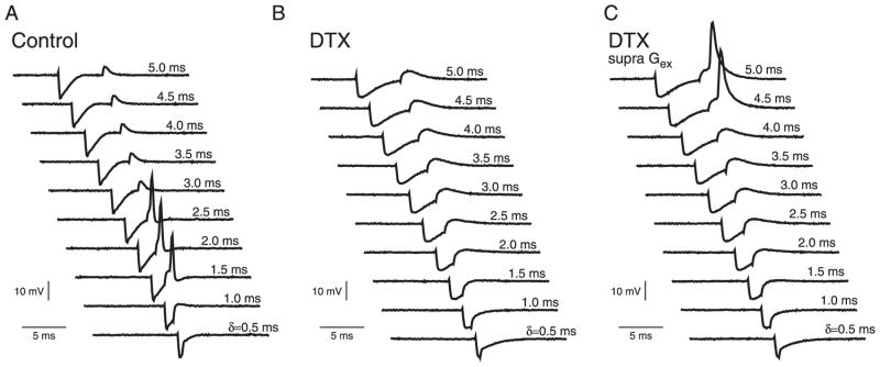
Experimental demonstration of postinhibitory facilitation. A: patch-clamp recordings (in vitro gerbil medial superior olive [MSO], P22) of membrane potential for a pair of inhibitory and subthreshold excitatory inputs, Gex = 20 nS, are applied with the dynamic-clamp method with varying preceding times of inhibition, Ginh = 100 nS, (see text for experimental details). B: elimination of PIF after application of the IKLT blocker dendrotoxin I (DTXI). Over the same range of δ as in A the inhibitory conductance transient (IPSG) does not facilitate the subthreshold excitatory conductance (EPSG) to generate a spike. C: Gex was increased by 5% relative to B for just-suprathreshold EPSG, which was preceded by an IPSG in the presence of DTXI. In all cases of the δ-range expected to show facilitation the IPSG suppressed spiking–no facilitation. To compensate for membrane conductance changes in B and C, the amplitudes of Gex and Ginh were reduced approximately 2-fold from the control conditions.
The PIF window depends on τinh
The IPSG’s (alpha function) time constant, τinh, plays an important role in positioning the PIF window. The IPSG’s peak value Ginh is independent of τinh but the IPSG’s time integral increases linearly with τinh, and is equal to Ginhe τinh. For very short time constants, there is too little inhibitory current generated to adequately hyperpolarize the cell and deactivate gKLT—no PIF window appears (Fig. 3A). For larger τinh, however, more current is generated by the IPSG, the cell hyperpolarizes more, and consequently w falls well below its rest value. Subsequent to the IPSG the cell is hyperexcitable. If the membrane potential rises faster than w can recover then a brief subthreshold EPSG may cause the cell to spike. If the EPSG is delivered too late then no spike will occur, thereby defining the upper δ-value for the PIF window. If the EPSG is delivered too early, the membrane is still being actively hyperpolarized and shunted by the IPSG. To be effective, and for PIF to occur, an EPSG must wait until most of the IPSG has run its course. This explains why the onset time of the PIF window increases with τinh; the dependency is nearly linear (as we will discuss below). If τinh is too large, the slow decay of the IPSG and its shunting effect forces the recovery of V and w to proceed hand in hand, disallowing V to outrace the recovery of the deactivated w. Thus for large τinh there is no PIF window.
FIG. 3.

Characterizing the PIF window. A: PIF window (seen in Fig. 1A) plotted vs. τinh, the time constant of the inhibitory conductance for fixed Ginh = 100 nS. Value of w for any given τinh as a function of δ is shown by the intensity of the gray scale. Gex = 8.2 nS, τex = 0.3 ms. Other parameter values are as in Fig. 1. Time window shown in Fig. 1A is indicated here by arrows. B: synaptic threshold (minimum Gex required to evoke a spike) in the PIF window shown in A for 2 values of τinh. Horizontal arrow next to the vertical axis shows the level of Gex used in A. Value Gex,rest corresponds to the threshold value of Gex for generating a spike from the rest state. C: response of the 5-variable model to brief inhibition alone, projected onto the V–w phase plane (for the same parameters as in A) for 4 values of τinh. Susceptible segments for evoking a spike for subthreshold excitation (when given as in A) are marked as thick lines. Filled circles indicate the point at which the inhibitory conductance has fallen to 10% of its peak value. D: total intrinsic (nonsynaptic) resistance of the membrane vs. time for trajectories shown in C. Dashed curve is the resistance arising from the synaptic inhibition alone. Filled circles indicate the same temporal positions as in C.
Within the PIF window, the degree of hyperexcitability is not uniform (Fig. 3B). The minimum strength of an EPSG to cause a spike depends on δ, approaching Gex,rest (the from-rest threshold value) as δ becomes large, and rising to a vertical asymptote as δ becomes small. The just-adequate EPSG strength (Gex value at the curve’s minimum) for PIF increases with increasing τinh (except for very small τinh). These plots show how the δ-range for PIF varies, widening and its upper boundary increasing as Gex increases. However, the dominant factor for positioning the PIF window is the time constant for the IPSG.
The interplay between the opposing factors for PIF, hyper-polarization (with V further from threshold) and deactivation of gKLT (hyperexcitability), may also be visualized with the help of phase-plane plots. In Fig. 3C we show projections from the five-variable model onto the V–w plane of the trajectories for the cell response to a single IPSG, for different values of τinh. The EPSGs are not included or needed here to illustrate the basic points; their associated EPSPs would overly complicate these images. A trajectory begins and ends at the rest state, with the flow direction being counterclockwise. The initial phase when the IPSG is applied shows hyperpolarization and then reduction in w. Because w lags behind V, the minimum in w occurs after the minimum in V. The dot indicates when the IPSG is essentially complete and it has fallen to 10% of its peak value. Before the dot, gsyn is strong and the net input resistance is reduced (below its resting value), enough to preclude a spike response to the EPSG. After the dot the PIF window is open, indicated by the heavy portion of a trajectory for the given amplitude of excitation Gex that was used for Fig. 3A. Later, as V and w are recovering to near their rest levels the window closes and the EPSG would not lead to a spike. We see here that the longer τinh is, the farther the PIF window migrates along the trajectory. For brief τinh the window opens even before gKLT is maximally deactivated. Note that for a fast-decaying IPSG the trajectory after the dot is basically reflecting the free (unstimulated) membrane’s subthreshold dynamics. Late in the time course all the trajectories return to the rest state, converging onto a common path and reflecting the eigenstructure for small deviations away from rest (see next section). For long τinh the slow decay means that there is still some residual synaptic conductance competing with the hyper-excitability and even some recovery of the also deactivated delayed rectifier conductance. Corresponding to the deactivation of gKLT the cell’s instantaneous (intrinsic, i.e., nonsynaptic) input resistance is transiently increased (Fig. 3D), contributing to the PIF by enhancing the depolarization from an EPSG. Because gK constitutes about 10% of the resting conductance its dynamics also contribute some degree (although much less than gKLT) to hyperexcitability and these input resistance time courses show the combined effects.
Let us consider a bit more the timing of when the PIF window opens. In Fig. 3, C and D we associated this opening with near completion of the inhibitory conductance transient; i.e., when ginh(t) had fallen to a small fraction, say ε, of its peak level Ginh. Before this time the shunting effect of the inhibitory conductance dominates the excitatory input. Therefore we estimate roughly the minimum δ when PIF first becomes available from the condition (recalling our notation in Eq. 3) Ginh(t0 − δ + δmin) = εGinh, i.e.
After canceling Ginh we see that this equation defines the value δmin/ τinh as some constant, depending only on the criterion level ε. Thus we have that δmin is approximately proportional to τinh.
Reduced V–w model
We have argued that IKLT is the dominant factor that under-lies PIF in the model. This view is based on the contention that the gating variables n and h are recruited only at higher voltages, and do not come into play until the membrane has reached threshold and spike initiation is proceeding. Here, we show this more convincingly by implementing the contention explicitly in a reduced model that retains only the dynamics of V and w. We simulate and analyze the two-variable model, highlighting the important features that contribute to the PIF effect. For the reduced model we freeze h and n at their resting values (h0 and n0, respectively) and we exploit the fact that sodium activation responds very rapidly to changes in V, approximating its dynamics as instantaneous, setting m = m∞(V). This reduced two-variable model reproduces semiquantitatively the subthreshold PIF behavior. It is valid for approximating a spike’s upstroke but it does not apply for the transient depolarized phase of an action potential or for the spike’s repolarization. In fact, for the control parameter values the reduced model does not repolarize, but with sufficient stimulus to provoke an upstroke the membrane potential latches up to a steady depolarized level because sodium inactivation and the delayed-rectifier potassium activation are frozen. The equations for the reduced V–w model are expressed as
| (4) |
| (5) |
where . The parameter values, resting potential (about −60 mV), and form of synaptic input current, Isyn, are identical to those of the previous sections. The PIF effect occurs as before (Fig. 4A): when inhibition falls within an optimal time window ahead of the subthreshold excitation, a spike (upstroke) is elicited. Here we use weaker synaptic conductances than for the full model. The V–w model is more excitable because the delayed rectifier is frozen and an upstroke is easier to attain. The PIF window for the reduced model, as for the full model, shows a similar dependency on τinh with the elliptical closed region in the (τinh, δ) plane (compare Fig. 4B with Fig. 3A) and the window’s onset value of δ increasing almost linearly with τinh. The reduced model shows similar dependencies of the PIF window on Gex as in the full model. The window enlarges with Gex (two cases shown in Fig. 4B; also compare Fig. 4C with Fig. 3B). The PIF window’s offset value depends sensitively on Gex (not shown, but similar to Fig. 1D). These simulation results demonstrate that the reduced V–w model well represents the significance of IKLT as a primary factor in PIF in the Rothman et al. (1993) model.
FIG. 4.

Reduction of the full 5-variable model to a 2-variable V–w model by freezing h and n and setting m = m∞(V). A: voltage time courses of the reduced model when a subthreshold EPSG is applied to the resting membrane at t = 50 ms and a preceding IPSG occurs at time 50-δ ms for various values of δ. Strong depolarizing response (a transition to a depolarized steady state in this bistable reduced model) approximates a spike upstroke for a range of δ values (shaded region). Parameters are identical to those in Fig. 1 except here Gex = 3.31 nS. B: PIF window is plotted as a function of τinh. Arrows correspond to the shaded PIF window in A. A reduced value of Gex reduces the size of the PIF window. Corresponding PIF window of the full model from Fig. 3A is replotted (dashed) for comparison. C: synaptic threshold for an upstroke plotted vs. δ for 2 values of τinh. Two horizontal arrows next to the vertical axis show the level of Gex for the two PIF windows shown in B. D: phase plane portraits of the V–w model showing the V- and w-nullclines, and the threshold separatrix (unique trajectories that enter the saddle point, from above and below; with double arrowheads). Inset: bird’s eye view, showing all 3 fixed points of the reduced system. Main panel shows the 2 trajectories corresponding to δ = 1 ms and 5 ms (from A). Filled circles on the trajectories mark the initiation of EPSGs, and the open circles denote the system’s state after each EPSG has fallen 80% from its peak level. The spike upstroke trajectory of PIF shows that system has crossed the threshold separatrix during delivery of the delayed excitation.
Because the reduced model has only two variables we can gain further insight into its properties by analyzing it in the phase plane. As in many models of membrane excitability with a fast-activating inward current and slower-activating outward current we find the familiar cubic V-nullcline and the sigmoidal w-nullcline (Koch 1999; Rinzel and Ermentrout 1998) (Fig. 4D, inset). In our case, because we have frozen the negative-feedback variables, h and n, the nullclines have three intersections, i.e., the system has three steady states. The lower V state corresponds to the rest state and the upper V state is the “excited” state, where the upstroke terminates. The “middle” steady state is a saddle point and determines the threshold characteristics. A magnification of the phase plane (Fig. 4D, main panel) better shows the subthreshold and upstroke behavior. There are two trajectories (double arrowheads) that exactly enter the saddle point, one from above and one from below; this latter trajectory, called the threshold separatrix (FitzHugh 1955), segregates state points from which the response evolves to the resting state or to the excited state. If after a transient input the system finds itself rightward of this separatrix a spike upstroke occurs. The V–w trajectories for two responses from Fig. 4A are shown in Fig. 4D; the flow is counterclockwise, reminiscent of Fig. 3C, but here we can also see the trajectories in relation to the nullclines and the separatrix (not possible for the two-variable projection of Fig. 3C from a five-variable phase space). After the brief excitatory input is essentially complete (marked by an open circle) the system is sitting below threshold in the case δ = 1 ms and above threshold for δ = 5 ms. Note that the positive slope of the separatrix reflects that (in the range being viewed) the distance from Vrest to threshold decreases for lower values of w, a geometric or phase plane correlate of hyperexcitability. Thus in the case of the upstroke trajectory, the EPSG is delivered after the IPSG is complete when (coincidentally) V ≈ Vrest and the membrane is hyperexcitable, so that a spike is evoked.
Rebound excitation after long or brief hyperpolarization; geometric treatment for V–w model
As one should expect, the reduced model’s applicability has a limited quantitative range. It works well for the qualitative feature of PIF, considering the responsiveness of priming transient inhibition. In this case the hyperpolarized levels do not fall below Einh (−66.5 mV). For stronger hyperpolarizations, say in response to Iapp steps, the V–w model, unlike the full model, predicts classical PIR. This can be understood from looking at a zoom-out of the phase plane (Fig. 5A). Here we see as we move away from the saddle point along the threshold separatrix that it makes a U-turn, crossing the w-nullcline at V ≈ −65.6 (see arrow) and exiting this zoom-out’s left border near w = 0.4. Now, for setting up conditions for PIR, suppose that a long hyperpolarizing current step is applied. Then the state point approaches a holding steady state with V and w that must lie along the w-nullcline, below rest. If this holding level has V less than −65.6 mV then the state point is below the threshold separatrix and when the current step is ended an upstroke (i.e., PIR) occurs. The full model does not show PIR for release from any maintained current steps. This is because n is not frozen and τn is small enough so that when V begins increasing on release and it increases beyond Vrest the n-gates open rapidly, more than at rest (the frozen level in the V–w model), and thereby preclude a spike. If n is adequately slowed by increasing τn artificially enough the full model does show PIR. The sensitivity of PIR to the degree of IK activation around rest is also somewhat reflected in the V–w model. For example, if the frozen value n0 were increased from 0.0194 to 0.05 (still only 5% activation) PIR would not occur in the V–w model. The separatrix would not cross the w-nullcline (Fig. 5B) and the reduced and full models would agree in this regard, as well as for PIF.
FIG. 5.
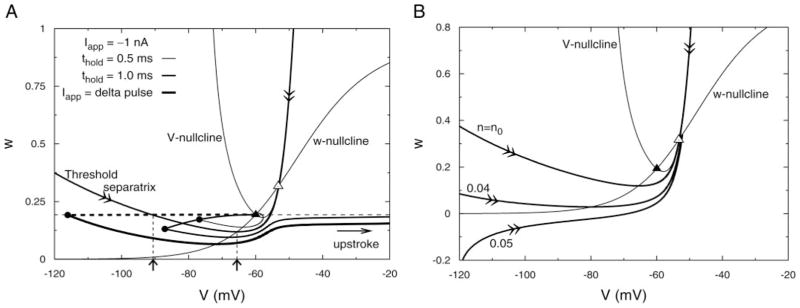
Reduced V–w model showing postinhibitory rebound after brief inhibition. A: phase plane (magnified) of the V–w model is shown along with its nullclines and the threshold separatrix. With n frozen at its resting value (same for h) the trajectory along the threshold separatrix is not monotonic in w. It crosses the w-nullcline when its w value is a minimum and it crosses the line w = wrest (see 2 up-arrows below horizontal axis). Therefore a strong hyperpolarizing delta pulse of negative current that instantaneously hyperpolarizes the membrane (thick dashes) leftward beyond the threshold separatrix gives rise to a postinhibitory rebound upstroke. Other 2 trajectories show responses for −1 nA when the current is briefly held steady for 1.0 ms or 0.5 ms, the latter being insufficient to induce a rebound upstroke. B: threshold separatrix is sensitive to the frozen value of n. Here, it is shown when n is set at its rest value of 0.0194 (as in A) and when n is held at 2 other small values: 0.04 and 0.05. With n frozen at the higher value, the separatrix is monotone in w, demonstrating that an elevated value of n suppresses the postinhibitory rebound (PIR) effect seen in A. Top branches of the separatrices and the corresponding nullclines for these 3 frozen values of n do not differ much, so they are omitted for clarity.
The V–w model is quite responsive to such strong hyperpolarizing inputs, even if they are very brief. For example, a 1-ms (1-nA) anodal current of a given amplitude is adequate to cause a rebound upstroke (Fig. 5A), although a briefer input of 0.5 ms is not. However, a briefer hyperpolarizing current step if made very strong can lead to rebound. In the extreme case of a delta-function of Iapp the membrane is instantaneously hyperpolarized and if this V-displacement below rest is large enough [here, ≲ −90.8 mV (see arrow), just leftward of where the threshold separatrix crosses upward through w = wrest] then rebound occurs (Fig. 5A). In this case of such a U-turning separatrix, the cell model behaves as if it had two thresholds for brief Iapp inputs: one for depolarizing pulses and one for hyperpolarizing pulses. The observation that a strong instantaneous hyperpolarizing current pulse can evoke a rebound spike was reported by FitzHugh for the classical HH model (FitzHugh 1976); here, by showing it in a two-variable model, we provide a geometric phase-plane interpretation (see also Izhikevich 2001).
Integrate-and-fire model with dynamic accommodating threshold
Until now we have focused on a biophysical mechanism for PIF and hyperexcitability, transient deactivation of a voltage-gated potassium current mediated by brief inhibition. This is a particular instantiation of the general mechanism that underlies PIF, a transient decrease in effective threshold by hyperpolarization. Next we implement this idea explicitly in a bare-bones model, an enhanced leaky integrate-and-fire (LIF) model.
Here, PIF does not depend on a conductance mechanism per se. In this minimal model the voltage threshold is a dynamic variable θ(t), which increases with depolarization and decreases with hyperpolarization with a time constant, and which can be chosen to be faster or slower than the membrane time constant. The dynamic behavior of θ represents an idealized form of accommodation [in the spirit of Hill (1936) and others (see Rashevsky 1960)]. Transient, even brief, synaptic inhibition and hyperpolarization causes θ(t) to decrease, inducing hyperexcitability. The model’s equations in dimensionless form are
| (6) |
| (7) |
Voltagelike quantities (v and θ) are expressed relative to rest and scaled by a reference voltage. Timelike quantities (e.g., t and δ) are scaled by the membrane time constant; i0 sets the resting or holding voltage and θ0 determines the resting level of threshold. The synaptic current is given by isyn = gex(t)(v − 2)+ ginh(t)v, where the synaptic conductances have the same functional form as in Eqs. 2 and 3; here, inhibition is pure shunting, although this aspect is not crucial. As in standard LIF models, v is reset to some subthreshold level (say, v = 0) when v reaches θ and a spike event is recorded. Note, this LIF-θ model is distinct from most other LIF models with variable threshold (or processes that affect threshold) that are meant to describe refractoriness and spike-frequency adaptation. In the latter, threshold depends on spiking but not typically on sub-threshold V(t) (see, e.g., Dayan and Abbott 2001; Liu and Wang 2001; but also Perkel et al. 1981).
Our idealized LIF-θ model indeed shows the PIF effect (Fig. 6, A and B). If excitation occurs too soon after inhibition the subthreshold EPSG is disadvantaged rather than facilitated. However, if the inhibition is delivered within a proper preceding time window then facilitation and a spike occurs. As in the previous models the PIF window’s position slides to greater δ as τinh increases (Fig. 6C). As we did for the V–w model we can analyze this two-variable LIF model in the phase plane (Fig. 6D). The nullclines and all behavior for v < θ are linear. The trajectories for two cases, analogous to those in Fig. 6, A and B, show the expected counterclockwise flow with the threshold being reduced, and reaching a minimum as the θ-nullcline is crossed. When δ is too small the state point is still “below” (to the left of) the “firing line” just after the excitatory input, so no spike occurs. Waiting a bit longer (δ somewhat larger but not by too much) means that the excitatory event pushes the system rightward over the firing line.
FIG. 6.

Leaky integrate-and-fire model (Eqs. 6 and 7) with an accommodating threshold shows PIF. A: time courses of voltage and of the voltage-dependent threshold θ plotted when an excitatory synaptic conductance (Gex = 0.05, τex = 0.1) is activated at t = 8, and an inhibitory conductance (Ginh = 5, τinh = 0.3) is activated at t = 5 (i.e., for δ = 3). Threshold is well above the evoked depolarization, and the cell does not fire. All variables are dimensionless. B: same as in A but with δ = 5. Hyperpolarization caused by the inhibition lowers the threshold that helped the well-timed excitation to push the voltage beyond the threshold, thus evoking a spike that is equivalent to the PIF effect shown by the full and reduced models illustrated in the previous figures. Dashed portions are afterspike time evolutions of V and θ. C: PIF window as a function of τinh (α = 0.3, θ0 = 0.09, i0 = 0.1, and τθ = 2). D: orbits of the nonfiring and firing cases seen in A and B plotted in the V–θ phase plane. Dashed portion is the afterspike evolution of the trajectory. A spike is evoked when the trajectory crosses the voltage-dependent threshold.
We can say more about this idealized two-variable model. Its eigenvalues are: −1 and −1/τθ; here, the rest or holding state does not have spiral structure. If θ lags behind v (τθ > 1) then the decay back toward the holding state from hyperpolarizing input ultimately will have its trajectory in the phase plane becoming tangent to the v-nullcline. That is, the eigenvector associated with the slower decay exp(−t/τθ) is vertical; consequently, there can be no overshoot of V in this model after inhibition. From the geometrical perspective we can also see how the competing factors of hyperpolarization and hyperexitability determine where along the return-to-rest trajectory the maximal facilitation occurs. Suppose we ask: At each position along the trajectory after a priming inhibitory input what is the just-adequate value of a brief (delta-function) pulse of depolarizing Iapp (delivering charge Qex) that would displace the membrane potential across the firing line? The answer, for Qex at time δ, is given by the horizontal distance from the trajectory to the firing line (Fig. 6D). Because the firing line is sloped positively (slope = 1) and the ultimate approach to rest is vertical we can see that as we back away from the rest point (δ decreasing from large values) Qex decreases then reaches a minimum and increases again. The plot of Qex versus δ has the same shape as the plots in Figs. 3B and 4C.
This LIF-θ model shows PIR behavior and this may be seen as follows. Because the firing line has slope of 1, it will intersect the v-nullcline at a low value of θ. If a steady hyperpolarizing Iapp is strong enough, the prerelease steady state will lie at an even lower θ-level, down on the lower left of the θ-nullcline. Then, if τθ is large, the system on release will reach the firing line (a rebound spike) before θ has time to recover very much; in fact, there could be several rebound spikes before θ adequately recovers. One can easily identify the least negative steady Iapp that results in rebound on release, i.e., by finding which starting point on the θ-nullcline is closest to rest but still leads to PIR. Having identified this threshold for PIR from steady hyperpolarization we can conclude that the LIF-θ model also gives a rebound spike for a strong enough delta pulse of hyperpolarizing Iapp. By following backward in time along the threshold PIR trajectory we see that it will ultimately cross the horizontal line that passes through the rest state. The v-coordinate of this crossing point defines the hyperpolarization threshold for the delta pulse that could produce a rebound spike, analogous to what we saw previously with the V–w model. Finally, we note that the LIF-θ model can fire phasically. If α > 1, then the v- and θ-nullclines will intersect only to the left of the firing line for any level of steady depolarizing Iapp. Thus after the step is applied, the system’s trajectory will go to this target, maybe hitting the firing line a few times beforehand (phasic firing); the larger the value of τθ, the more spikes will occur during this transient phase.
PIF for periodic inputs
Until this point we have considered PIF as it occurs for an IPSG–EPSG input pair. The essential mechanism that we have identified is also observable in the responses to longer input trains. Here we illustrate the PIF phenomenon for periodic trains of synaptic inputs, EPSG trains and IPSG trains of the same period but phase-shifted. The in vitro recording of an MSO neuron (Fig. 7A) shows facilitation when a phase-locked train of IPSGs is presented with a periodic train of subthreshold EPSGs and the phase difference is in an appropriate range. In the absence of inhibition, the pure EPSG train elicited no spikes (Fig. 7A, bottom trace). The spiking, arising from PIF, occurred with multiple ratios of frequency locking, but predominantly 1:1. Computations with the full model show PIF for phase-locked periodic inputs for a range of δ/T values and for various frequencies (Fig. 7, B and C). For any periodic train of combined inputs, IPSG–EPSG pairs occur automatically with the same frequency as that of the input. If a single pair results in a spike by PIF, the combined input will now result in 1:1 firing as long as the input period is sufficiently longer than the refractory period. As the input frequency increases, the refractory period begins to overlap with the time window necessary for PIF spike production. This prevents some IPSG–EPSG pairs from producing a spike. Thus for increased input rate, the firing ratio falls below 1:1. In Fig. 7C the dominant spike mode is 1:1 for 100-Hz input, but for a 200-Hz input the ratio is almost totally 1:2.
FIG. 7.

PIF occurs for periodic inputs in experiments and simulations; in the model, for extended parameter regimes: τinh slower (≤3 ms, from previously <1 ms) and weaker inhibitory strengths. A: recordings of an in vitro MSO cell for periodic trains of EPSGs and phase-shifted IPSGs for different phase shifts measured with respect to the input period at 200 Hz; the relative phase shift is δ/T. Bottom trace: response, nonspiking, for pure subthreshold periodic excitation. For a particular range of δ/T inhibition facilitates firing. Inputs (delivered with the dynamic-clamp method) are pure exponential functions with Gex = 40 nS, Ginh = 100 nS. B: computed voltage responses of the complete model (Rothman et al. 1993) showing phase- and frequency-locked spiking for inputs similar to those in A. Inputs are modeled as alpha functions (τinh = 0.3 ms) with rate 150 Hz; all other parameters are the same as in Fig. 1A. C: computed PIF regions for input rates of 100 and 200 Hz for parameters as in Fig. 3A. Color coding in C–E indicates the firing rate of the membrane relative to the input rate. D and E: with enhanced leakage conductance (12.2 nS) and for inputs that are simple exponentials (not alpha functions) the model shows PIF for extended parameter ranges: longer inhibitory time constants and weaker synaptic strengths. In D the PIF region in the (δ/T, τinh) parameter plane extends up to τinh = 3 ms, for these frequencies, 100 and 200 Hz. Note, the relative phase shifts for the PIF range correspond to absolute time differences between inhibition and excitation, say for 100 Hz, of 0.5 to 2.5 ms, considerably less than those in Fig. 3A. Here, Gex (15.6 nS) is 20% below the threshold value for a single excitatory input to generate a spike. In E the PIF regions are shown in (Ginh, δ) space for τinh = 2 ms. Facilitation occurs for Ginh values as low as 15 nS (or smaller); in this regime an isolated inhibitory transient input hyperpolarizes the membrane only 1.6 mV (or less).
In the context of this periodic stimulation protocol we further explore some parameter dependencies. The PIF regions in Fig. 7C (and in Fig. 3A) are for τinh <1 ms, primarily because of the fact that the membrane time constant and τw are small, say ≤2 ms. Also, in the application of this model to MSO ITD tuning, Brand et al. (2002) used τinh = 0.1 ms. This value is extremely short even when compared to some of shortest inhibitory decay time constants reported for auditory brain stem (Awatramani et al. 2004). Recent estimates for the glycine-mediated inhibition in MSO place τinh around 2 ms (Magnusson et al. 2005). By making modest modifications to the model we have extended upward the range of τinh for PIF. For the results in Fig. 7, D and E we increased the leakage conductance and used a fast-rising ginh(t) (instantaneous) with a pure exponential decay rather than an alpha-function time course. The primary effect of using the exponential ginh(t) is that the absolute phase shift δ is smaller (Fig. 7D) than that in Fig. 7C: ≤3 ms for 100-Hz input and ≤4 ms for 200-Hz input. For this case, Gex is 20% below the threshold value for spike generation from a single EPSG, and Ginh is 25 nS. Figure 7E illustrates the PIF region in the (Ginh, δ) plane for τinh = 2 ms and two input frequencies, 100 and 200 Hz. The enhanced leakage conductance allows PIF to occur for Ginh values as low as 15 or 10 nS. This region is robust with respect to variations in Gex (data not shown).
DISCUSSION
Brief, well-timed inhibition can induce a spike-generating response to a subsequent, otherwise subthreshold, excitatory synaptic input. The brief inhibition leads to a transient phase of hyperexcitability. The trade-off between hyperpolarization and hyperexcitability leads to a specific time window for the postinhibitory facilitation, PIF. This window’s width (possibly quite narrow) and temporal position are determined by the membrane time constant and that of the subthreshold negative feedback that underlies PIF. The PIF window’s onset time increases with τinh and its width/size increases with the excitatory synaptic strength. The PIF phenomenon in its simplest form is for an inhibitory– excitatory pair but the effects are also seen in longer trains. Our findings suggest that patterns of inhibition–(subthreshold) excitation timing can increase firing probability beyond that from just temporal summation of subthreshold excitation.
We demonstrate PIF here with a case study: experimentally, in MSO neurons in vitro and in a conductance-based model (Rothman et al. 1993), dissecting the latter to analyze the mechanism. In this system brief inhibition transiently decreases a low-threshold potassium conductance, below its partially activated level at rest. The basic mechanism of fast inhibition leading to temporary reduction of a subthreshold negative feedback is quite general. We formulate two different simplified two-variable models and demonstrate, with simulation and phase plane analysis, the essential and qualitative features of PIF. Both of these reduced models also show PIR. Moreover, they can rebound with a spike for extremely brief hyperpolarizing current injection, suggesting that some neurons have two thresholds for input pulses, depolarizing and hyperpolarizing.
Biophysical factors that affect PIF
A number of factors influence the PIF effect and the window for facilitation, its width and position. We have shown (Figs. 3A, 4B, and 6C) that the window’s onset time increases with the IPSG’s time constant τinh. The onset time also depends on the time constant for the determining subthreshold negative feedback. This time constant (together with the membrane time constant) influences the membrane’s intrinsic dynamics during the recovery after synaptic inhibition, i.e., during the phase of hyperexcitability. In the five-variable model, and in our reduction of it, τKLT sets the scale of a few milliseconds for the window’s onset; τθ is the analogous factor in the LIF-θ model. More generally, other dynamic negative feedback processes could contribute to PIF. For example, if INa is partially inactivated at rest then reducing this inactivation by transient hyperpolarization could be a significant player in the integration of subthreshold inputs (Svirskis et al. 2004) and PIF, and then τh would influence the PIF timescales. In the full model (Rothman et al. 1993) INa inactivation (h) and IK activation (n) are secondary to IKLT gating for PIF. However if, say, IKLT were blocked or w were frozen in the full model then n-dynamics would play a dominant role (not shown here). The onset time of the PIF window would be reduced, down to a millisecond or so, because τn is much smaller than τw. As we have shown, the offset time of the PIF window increases with the EPSG strength, in each of the models that we have discussed.
PIF and subthreshold dynamics
If the time constants of the subthreshold negative feedback are too fast compared with the membrane time constant we would not observe PIF; the hyperexcitability phase would end too soon. If too slow then brief hyperpolarization will not enable hyperexcitability to appear. When, say, τKLT is not too different from the membrane time constant, however, then we find an opportunity for a PIF window for some IPSG and EPSG amplitudes. The important point is the dynamic interplay between V and the subthreshold process that induces hyperexcitability. This interplay is visualized as the counterclockwise flow in our phase-plane views (it would look clockwise in the V–h plane if INa inactivation were the dominant factor). Various transient inputs can push the system into this region of phase space and onto a trajectory that contains a PIF window. It would be an oversimplification to say that PIF occurs only if the subthreshold behavior involves a strictly spiraling-like behavior after transient perturbing inputs. Although subthreshold (damped) resonance is sufficient (see also Izhikevich 2001), and might even result in spike “probability oscillation” after an inhibitory input in a stochastic background (Luk and Aihara 2000), it is not necessary for PIF. Our LIF-θ model shows PIF behavior but the ultimate trajectory in returning toward rest is not spiral, and V does not overshoot Vrest.
Beyond specified pairings
In most of our illustrations of PIF the input was an IPSG-then-EPSG input pair with specified timing. However, the essential mechanism is general and also underlies enhancement effects of spiking for longer input trains and with temporal ordering unspecified. We illustrated (Fig. 7) the PIF phenomenon for periodic trains of synaptic inputs, EPSG trains and IPSG trains of the same period but phase-shifted. Although we understand the enhancement of firing by considering the effect of an IPSG priming the membrane for hyperexcitability for a succeeding EPSG the notion of which PSG leads is not obviously a priori meaningful for periodic inputs. More generally, for input trains with randomly arriving EPSGs and IPSGs some PIF-favorable timings will occur by chance. Indeed, our simulations with the classical HH model show that introducing random, fast IPSGs to a train of subthreshold EPSGs enhances the spontaneous firing rate. Identification of spike-triggered synaptic events reveals the enhancement in firing is attributed to timely IPSG–EPSG pairings (Dodla and Rinzel 2006).
Delivery and release rate of hyperpolarization
Even very, very fast hyperpolarizing input can induce PIF. For our V–w and LIF-θ models we saw that, in the extreme case of a delta-pulse input, we get essentially instantaneous hyperpolarization and the subsequent recovery trajectory not only contains a PIF window but, on its own, may lead to a rebound spike (Fig. 5). The geometrical (phase-plane) view enables us to see that for such a case of rebound spiking after a delta pulse that classical PIR (a rebound spike after release from adequate and steady Iapp < 0) was also guaranteed to occur. This is an interesting connection between the effect of long duration and very briefly applied hyperpolarization.
In either of these cases the hyperpolarizing stimulus is instantaneously terminated. This feature of classical PIR is sometimes overlooked. One should think more generally that a fast enough return to zero stimulus (Iapp = 0) is required to induce rebound (Ferragamo and Oertel 2002; Gutierrez et al. 2001). This necessity is consistent with our observations on PIF that ginh(t) must be fast enough (Figs. 3 and 7) and underscores, in particular, that the decay must be fast enough. If the stimulus relaxes too slowly the system would merely track the slowly recovering hyperpolarized state back to rest. The opportunity would be lost for exploiting the hyperexcitability and have V outrace the slightly lagging recovery of the negative feedback.
For the brain stem model we found PIF for τinh in the submillisecond (Fig. 3A) to millisecond (Fig. 7D) ranges. In the experimental/computational study of gerbil MSO ITD tuning (Brand et al. 2002) the modeling results were based on τinh = 0.1 ms. Recent patch-clamp data are finding in these neurons that τinh is closer to 2-ms (Magnusson et al. 2005). Such brief inhibition is not unique to the auditory system. In hippocampal slices τinh values of 2 ms or so have been reported (Bartos et al. 2002).
The reduced V–w model
The saddle-point threshold behavior visualized in the phase plane of Figs. 4D and 5, A and B is not necessary for PIF behavior, but this instantiation of excitability enables a clear understanding. Moreover, similar geometry is common to a class of neuronal models and therefore supports the generality of our findings for the illustrative case study from the auditory brain stem. This same geometry and similar behaviors are obtained for a two-dimensional reduction of the classical HH model with m = m∞(V) and h frozen at its rest value (Dodla and Rinzel 2006).
We note here that our formulation of the reduced V–w model was not based on a mathematical derivation from the full model of Rothman et al. (1993). Usually such reductions lean on timescale differences in dynamic processes: e.g., allowing fast variables to track instantaneously quasi-steady-state values [as we did, by setting m = m∞(V)] or by fixing slow variables to their values at a rest or holding state. In our case, we ignored the dynamics of h and n by noting that they were not significant players as dynamic negative feedback in the subthreshold voltage range; this simplification proved reasonably successful for addressing some issues, such as responses to IPSGs and EPSGs. Interestingly, in this model n is noticeably faster than w for V < Vrest; it is just very small. This leads us to caution that assessing the contribution of various gating factors to subthreshold integration depends not only on their V-dependent gating amplitudes but on the V dependency of their time constants. In some cases the tail-end values of the typically bell-shaped V dependency of τ (or the atypically shaped profiles of τh and τn in this model) may be near zero and so the identification of fast/slow timescales requires careful consideration.
Timed inhibition and coding
In considering a system’s temporal coding properties one often asks about the precision in detecting nearly coincident subthreshold excitatory inputs. Interestingly, as we have shown here, the same intrinsic biophysical factors that contribute to high-fidelity coincidence detection in the auditory brain stem case endow the neurons with enhanced firing probability for precise and preferred timing between subthreshold excitation and preceding brief inhibition. Although timed and fast inhibition plays a role in temporal processing and ITD tuning in the gerbil MSO (Brand et al. 2002; Grothe and Sanes 1994) the evidence at this point suggests that the contribution there is to reduce firing to deselect some ITDs and create asymmetry in the tuning curve. Whether PIF plays a role in ITD sensing by MSO or in other signal processing by auditory brain stem remains to be seen. Nevertheless, other timing computations in the auditory system involve transient inhibition that precedes excitation. In the bat auditory system delay sensitivity (for outgoing and incoming sonar signals) is seen in some neurons in the cortex and inferior colliculus. Localized pharmacological blocking of transient inhibition onto these cells degrades or eliminates the delay-sensitive firings (Wenstrup and Leroy 2001). Bat IC neurons that show sensitivity to sound duration are also seen to fire for appropriately timed (otherwise subthreshold) excitation after offset of inhibition (Casseday et al. 1994; Covey and Casseday 1999; Covey et al. 1996). Although the absolute timescales of biophysical mechanisms are longer in higher structures such as IC than in MSO, it is the relative values that determine whether PIF might occur. The mechanism that we describe here is a viable candidate for such phenomena. Our modeling results, especially for the reduced models, suggest that postinhibitory facilitation is a quite general feature. Even for random inputs one can expect favorable timings for PIF to occur by chance, thereby providing a contribution to spontaneous activity (Dodla and Rinzel 2006). Surely many neural systems for implementing computations can take advantage of the synergy between transient subthreshold excitation that is primed by relatively brief or rapidly decaying timed inhibition.
Acknowledgments
The authors are grateful to the Mathematical Biosciences Institute at Ohio State University (http://mbi.osu.edu/) for providing support and a stimulating environment during and following a workshop on the Auditory System (May 2003) when many of the ideas and results presented here were developed.
GRANTS
This research was supported by funding from National Institute of Mental Health Grant MH-62595.
APPENDIX
The voltage dependencies of the rate constants αx and βx of the full model described in the paper, identical to those used by Rothman et al. (1993), are listed below:
The conductances are given by GNa = 325 × Tf (2), GK = 40 × Tf (2.5), GKLT = 20 × Tf (2.5), and GL = 1.7 × Tf (2). The temperature factor is , where T = 38°C. Integration of the equations was done using a fourth-order Runge–Kutta method with a fixed time step of ≤0.01 ms. All the nullclines and separatrices in the phaseplanes were obtained using the software package XPPAUT (Ermentrout 2002).
References
- Awatramani GB, Turecek R, Trussell LO. Inhibitory control at a synaptic relay. J Neurosci. 2004;24:2643–2647. doi: 10.1523/JNEUROSCI.5144-03.2004. [DOI] [PMC free article] [PubMed] [Google Scholar]
- Bartos M, Vida I, Frotscher M, Meyer A, Monyer H, Geiger JRP, Jonas P. Fast synaptic inhibition promotes synchronized gamma oscillations in hippocampal interneuron networks. Proc Natl Acad Sci USA. 2002;99:13222–13227. doi: 10.1073/pnas.192233099. [DOI] [PMC free article] [PubMed] [Google Scholar]
- Brand A, Behrend O, Marquardt T, McAlpine D, Grothe B. Precise inhibition is essential for microsecond interaural time difference coding. Nature. 2002;417:543–547. doi: 10.1038/417543a. [DOI] [PubMed] [Google Scholar]
- Casseday JH, Ehrlich D, Covey E. Neural tuning for sound duration—role of inhibitory mechanisms in the inferior colliculus. Science. 1994;264:847– 850. doi: 10.1126/science.8171341. [DOI] [PubMed] [Google Scholar]
- Covey E, Casseday JH. Timing in the auditory system of the bat. Annu Rev Physiol. 1999;61:457– 476. doi: 10.1146/annurev.physiol.61.1.457. [DOI] [PubMed] [Google Scholar]
- Covey E, Kauer JA, Casseday JH. Whole-cell patch-clamp recording reveals subthreshold sound-evoked postsynaptic currents in the inferior colliculus of awake bats. J Neurosci. 1996;16:3009–3018. doi: 10.1523/JNEUROSCI.16-09-03009.1996. [DOI] [PMC free article] [PubMed] [Google Scholar]
- Dayan P, Abbott L. Theoretical Neuroscience. Cambridge, MA: MIT Press; 2001. p. 165. [Google Scholar]
- Dodla R, Rinzel J. Enhanced neuronal response induced by fast inhibition. Phys Rev E. 2006;73:010903 (R). doi: 10.1103/PhysRevE.73.010903. [DOI] [PMC free article] [PubMed] [Google Scholar]
- Ermentrout B. Simulating, Analyzing, and Animating Dynamical Systems: A Guide to XPPAUT for Researchers and Students. Philadelphia, PA: Society for Industrial and Applied Mathematics; 2002. [Google Scholar]
- Ferragamo MJ, Oertel D. Octopus cells of the mammalian ventral cochlear nucleus sense the rate of depolarization. J Neurophysiol. 2002;87:2262–2270. doi: 10.1152/jn.00587.2001. [DOI] [PubMed] [Google Scholar]
- FitzHugh R. Mathematical models of threshold phenomena in the nerve membrane. Bull Math Biophys. 1955;17:257–278. [Google Scholar]
- FitzHugh R. Anodal excitation in the Hodgkin–Huxley nerve model. Biophys J. 1976;16:209–226. doi: 10.1016/S0006-3495(76)85682-2. [DOI] [PMC free article] [PubMed] [Google Scholar]
- Gardner SM, Trussell LO, Oertel D. Time course and permeation of synaptic AMPA receptors in cochlear nuclear neurons correlate with input. J Neurosci. 1999;19:8721– 8729. doi: 10.1523/JNEUROSCI.19-20-08721.1999. [DOI] [PMC free article] [PubMed] [Google Scholar]
- Gauck V, Jaeger D. The control of rate and timing of spikes in the deep cerebellar nuclei by inhibition. J Neurosci. 2000;20:3006–3016. doi: 10.1523/JNEUROSCI.20-08-03006.2000. [DOI] [PMC free article] [PubMed] [Google Scholar]
- Goldberg JM, Brown PB. Response of binaural neurons of dog superior olivary complex to dichotic tonal stimuli: some physiological mechanisms of sound localization. J Neurophysiol. 1969;32:613– 636. doi: 10.1152/jn.1969.32.4.613. [DOI] [PubMed] [Google Scholar]
- Granit R. Reflex rebound by post-tetanic potentiation: temporal summation—spasticity. J Physiol. 1956;131:32–51. doi: 10.1113/jphysiol.1956.sp005442. [DOI] [PMC free article] [PubMed] [Google Scholar]
- Grothe B. New roles for synaptic inhibition in sound localization. Nat Rev Neurosci. 2003;4:1–11. doi: 10.1038/nrn1136. [DOI] [PubMed] [Google Scholar]
- Grothe B, Sanes DH. Synaptic inhibition influences the temporal coding properties of medial superior olivary neurons: an in vitro study. J Neurosci. 1994;14:1701–1709. doi: 10.1523/JNEUROSCI.14-03-01701.1994. [DOI] [PMC free article] [PubMed] [Google Scholar]
- Gutierrez C, Cox CL, Rinzel J, Sherman SM. Dynamics of low threshold spike activation in relay neurons of the cat lateral geniculate nucleus. J Neurosci. 2001;21:1022–1032. doi: 10.1523/JNEUROSCI.21-03-01022.2001. [DOI] [PMC free article] [PubMed] [Google Scholar]
- Hill AV. Excitation and accommodation in nerve. Proc R Soc Lond B Biol Sci. 1936;119:305–355. [Google Scholar]
- Izhikevich EM. Resonate-and-fire neurons. Neural Networks. 2001;14:883–894. doi: 10.1016/s0893-6080(01)00078-8. [DOI] [PubMed] [Google Scholar]
- Koch C. Biophysics of Computation. New York: Oxford Univ. Press; 1999. [Google Scholar]
- Koch U, Grothe B. Hyperpolarization-activated current (Ih) in the inferior colliculus: distribution and contribution to temporal processing. J Neurophysiol. 2003;90:3679–3687. doi: 10.1152/jn.00375.2003. [DOI] [PubMed] [Google Scholar]
- Kuffler SW, Eyzaguirre C. Synaptic inhibition in an isolated nerve cell. J Gen Physiol. 1955;39:155–184. doi: 10.1085/jgp.39.1.155. [DOI] [PMC free article] [PubMed] [Google Scholar]
- Liu Y-H, Wang X-J. Spike-frequency adaptation of a generalized leaky integrate-and-fire model neuron. J Comp Neurosci. 2001;10:25– 45. doi: 10.1023/a:1008916026143. [DOI] [PubMed] [Google Scholar]
- Luk WK, Aihara K. Synchronization and sensitivity enhancement of the Hodgkin–Huxley neurons due to inhibitory inputs. Biol Cybern. 2000;82:455–467. doi: 10.1007/s004220050598. [DOI] [PubMed] [Google Scholar]
- Lytton WW, Sejnowski TJ. Simulations of cortical pyramidal neurons synchronized by inhibitory interneurons. J Neurophysiol. 1991;66:1059–1079. doi: 10.1152/jn.1991.66.3.1059. [DOI] [PubMed] [Google Scholar]
- Magnusson AK, Kapfer C, Grothe B, Koch U. Maturation of glycinergic inhibition in the gerbil medial superior olive after hearing onset. J Physiol. 2005;568:497–512. doi: 10.1113/jphysiol.2005.094763. [DOI] [PMC free article] [PubMed] [Google Scholar]
- Manis PB, Marx SO. Outward currents in isolated ventral cochlear nucleus neurons. J Neurosci. 1991;11:2865–2880. doi: 10.1523/JNEUROSCI.11-09-02865.1991. [DOI] [PMC free article] [PubMed] [Google Scholar]
- Perkel DH, Mulloney B, Budelli RW. Quantitative methods for predicting neuronal behavior. Neuroscience. 1981;6:823– 837. doi: 10.1016/0306-4522(81)90165-2. [DOI] [PubMed] [Google Scholar]
- Perkel DH, Schulman JH, Bullock TH, Moore GP, Segundo JP. Pacemaker neurons: effects of regularly spaced synaptic input. Science. 1964;145:61– 63. doi: 10.1126/science.145.3627.61. [DOI] [PubMed] [Google Scholar]
- Rashevsky N. Physico-Mathematical Foundations of Biology. Vol. 1. New York: Dover; 1960. Mathematical biophysics. [Google Scholar]
- Rathouz M, Trussell LO. Characterization of outward currents in neurons of the avian nucleus magnocellularis. J Neurophysiol. 1998;80:2824–2835. doi: 10.1152/jn.1998.80.6.2824. [DOI] [PubMed] [Google Scholar]
- Reyes A, Rubel EW, Spain WJ. In vitro analysis of optimal stimuli for phase-locking and time-delayed modulation of firing in avian nucleus laminaris neuron. J Neurosci. 1996;16:993–1007. doi: 10.1523/JNEUROSCI.16-03-00993.1996. [DOI] [PMC free article] [PubMed] [Google Scholar]
- Rinzel J, Ermentrout GB. Analysis of neuronal excitability and oscillations. In: Koch C, Segev I, editors. Methods in Neuronal Modeling: From Ions to Networks. 2. Cambridge, MA: MIT Press; 1998. [Google Scholar]
- Rothman JS, Manis PB. The roles potassium currents play in regulating the electrical activity of ventral cochlear nucleus neurons. J Neurophysiol. 2003;89:3097–3113. doi: 10.1152/jn.00127.2002. [DOI] [PubMed] [Google Scholar]
- Rothman JS, Young ED, Manis PB. Convergence of auditory nerve fibers onto bushy cells in the ventral cochlear nucleus: implications of a compartmental model. J Neurophysiol. 1993;70:2562–2583. doi: 10.1152/jn.1993.70.6.2562. [DOI] [PubMed] [Google Scholar]
- Segev I, Rall W. Computational study of an excitable dendritic spine. J Neurophysiol. 1988;60:499–523. doi: 10.1152/jn.1988.60.2.499. [DOI] [PubMed] [Google Scholar]
- Sharp AA, O’Neil MB, Abbott LF, Marder E. The dynamic clamp: artificial conductances in biological neurons. Trends Neurosci. 1993;16:389–394. doi: 10.1016/0166-2236(93)90004-6. [DOI] [PubMed] [Google Scholar]
- Spitzer MW, Semple MN. Neurons sensitive to interaural phase disparity in gerbil superior olive: diverse monaural and temporal response properties. J Neurophysiol. 1995;73:1668–1690. doi: 10.1152/jn.1995.73.4.1668. [DOI] [PubMed] [Google Scholar]
- Svirskis G, Dodla R, Rinzel J. Subthreshold outward currents enhance temporal integration in auditory neurons. Biol Cybern. 2003;89:333–340. doi: 10.1007/s00422-003-0438-2. [DOI] [PMC free article] [PubMed] [Google Scholar]
- Svirskis G, Kotak V, Sanes DH, Rinzel J. Enhancement of signal-to-noise ratio and phase locking for small inputs by a low-threshold outward current in auditory neurons. J Neurosci. 2002;22:11019–11025. doi: 10.1523/JNEUROSCI.22-24-11019.2002. [DOI] [PMC free article] [PubMed] [Google Scholar]
- Svirskis G, Kotak V, Sanes DH, Rinzel J. Sodium along with low threshold potassium currents enhance coincidence detection of subthreshold noisy signals in MSO neurons. J Neurophysiol. 2004;91:2465–2473. doi: 10.1152/jn.00717.2003. [DOI] [PMC free article] [PubMed] [Google Scholar]
- Svirskis G, Rinzel J. Influence of subthreshold nonlinearities on signal-to-noise ratio and timing precision for small signals in neurons: minimal model analysis. Network Comput Neural Syst. 2003;14:137–150. [PMC free article] [PubMed] [Google Scholar]
- Trussell LO. Synaptic mechanisms for coding timing in auditory neurons. Annu Rev Physiol. 1999;61:477– 496. doi: 10.1146/annurev.physiol.61.1.477. [DOI] [PubMed] [Google Scholar]
- Wang XJ, Buzsáki G. Gamma oscillation by synaptic inhibition in a hippocampal interneuronal network model. J Neurosci. 1996;16:6402– 6413. doi: 10.1523/JNEUROSCI.16-20-06402.1996. [DOI] [PMC free article] [PubMed] [Google Scholar]
- Wenstrup JJ, Leroy SA. Spectral integration in the inferior colliculus: role of glycinergic inhibition in response facilitation. J Neurosci. 2001;21:RC124, 1–6. doi: 10.1523/JNEUROSCI.21-03-j0002.2001. [DOI] [PMC free article] [PubMed] [Google Scholar]
- Whittington MA, Traub RD, Jefferys JGR. Synchronized oscillations in interneuron networks driven by metabotropic glutamate-receptor activation. Nature. 1995;373:612– 615. doi: 10.1038/373612a0. [DOI] [PubMed] [Google Scholar]
- Yin TC, Chan JCK. Interaural time sensitivity in medial superior olive of cat. J Neurophysiol. 1990;64:465– 488. doi: 10.1152/jn.1990.64.2.465. [DOI] [PubMed] [Google Scholar]