An Approach for Identifiability of Population Pharmacokinetic–Pharmacodynamic Models

Abstract

Mathematical models are routinely used in clinical pharmacology to study the pharmacokinetic and pharmacodynamic properties of a drug in the body. Identifiability of these models is an important requirement for the success of these clinical studies. Identifiability is classified into two types, structural identifiability related to the structure of the mathematical model and deterministic identifiability which is related to the study design. There are existing approaches for assessment of structural identifiability of fixed-effects models, although their use appears uncommon in the literature. In this study, we develop an informal unified approach for simultaneous assessment of structural and deterministic identifiability for fixed and mixed-effects pharmacokinetic or pharmacokinetic–pharmacodynamic models. This approach uses an information theoretic framework. The method is applied both to simple examples to explore known identifiability properties and to a more complex example to illustrate its utility.

Models are frequently used to study, understand, and quantify the relationship between the components of a biological system.¹ Mathematical models play an important role in systems biology to understand the underlying mechanisms such as physiological, pathological, and pharmacological responses. Examples of system models include the blood glucose model by Cobelli et al.,² the tumor growth model by Adam,³ and the humoral coagulation network model by Wajima et al.⁴ Identifiability of these models or reduced versions of these models is an important component in their application to modeling experimental results.

Application of mathematical models is routine in pharmacokinetics (PK) and in pharmacokinetic–pharmacodynamic (PKPD) studies. Estimation of unknown parameters in the model is a critical step in understanding the underlying exposure–response relationship and has an important role in decision making. A unique solution for the unknown parameters that links any set of inputs to a set of outputs is a critical requirement for any model-based analysis. Although this may be relaxed to a finite set of solutions in the special case of “flip–flop” PK.⁵ the process of assessing for a unique solution for the parameters is encompassed within the framework of identifiability analysis. Parameters in the model that are not identifiable, i.e., not able to be estimated, pose challenges during the estimation step, leading to both imprecise parameter estimation and misleading conclusions or failure of the modeling process. Issues with identifiability are often intuitive for simple models (e.g., attempting to estimate the bioavailable fraction for an orally administered drug when data are only available after oral administration) but not so obvious in the case of more complex models (see the work on ivabradine by Evans et al.⁶). Recent developments in PK, PKPD, and systems pharmacology have centered on the development of more mechanistic (and hence complicated) models, and it is likely that identifiability of these models may not be intuitive.

Various methods are available in the literature for assessment of identifiability of linear and nonlinear PK models.^7,8,9,10 Assessment of identifiability based on evaluation of the Jacobian matrix was investigated by Jacquez¹¹ and Jacquez and Perry¹² for fixed-effects models. Although these are a very important aspect of model validation as illustrated by Cobelli and DiStefano¹³ and Yates et al.,¹⁴ identifiability analyses are often not practiced routinely, which may be due to the complexity of the mathematical computation involved in its execution or ease of availability and use of software. Bortz and Nelson¹⁵ briefly mentioned the importance of identifiability analysis in their work on mixed-effects modeling of and model selection for HIV infection dynamics.

Clinical studies are now more often analyzed using a population analysis approach.¹⁶ Population models are encompassed within the framework of nonlinear mixed-effects models that have natural hierarchies. It is desired in a population-based approach that all of the underlying parameters (fixed and random-effects parameters) are identifiable and should have an expected reasonable precision in their estimates. Currently, existing approaches to identifiability focus on identifiability of the fixed-effects parameters, and no specific approaches have been proposed to formally study the identifiability of random-effects parameters in population models. An exploration of this area in PK was recently proposed by Knutsson and Aarons.¹⁷

Identifiability of models is classified into two types: structural and deterministic identifiability. Structural identifiability, also termed a priori identifiability, is related to the structure of the underlying mathematical model and reflects whether the parameters in the assumed model have a unique solution given perfect input–output data. Structural identifiability classifies a model into any one of the three following subtypes:

1. Structurally globally identifiable: All parameters in the model have unique solutions.

2. Structurally locally identifiable: One or more parameters in the model have a finite number of alternate solutions.

3. Structurally unidentifiable: One or more parameters in the model have an infinite number of alternate solutions.

Deterministic identifiability, also termed a posteriori identifiability or practical identifiability¹⁸ or numerical identifiability,¹⁹ relates to the informativeness of the data and is influenced by the study design and its execution. Deterministic identifiability deals with assessment of whether the parameters in a model can be estimated precisely given imperfect input–output data. In its most basic form, deterministic identifiability requires that the number of observations (n) is greater than or equal to the number of unknown parameters (p). Of note, all structurally unidentifiable models are deterministically unidentifiable, whereas a structurally identifiable model need not be deterministically identifiable. Although few software tools^20,21 were designed to assess the structural identifiability, no dedicated software is available to assess deterministic identifiability. However, any software that has been developed for an optimal design of experiments^22,23 can be used to explore the deterministic identifiability.

The purpose of this paper is to develop and evaluate a unified approach for identifiability analysis of both fixed and mixed-effects PKPD models that encompasses both structural and deterministic identifiability. Note here we only consider PK models, but the methods are also applicable to PKPD models. The proposed approach is described in the following theory section. Furthermore, we provide the results for three specific objectives and a general discussion. The specific objectives are (i) to evaluate the method for assessing identifiability for simple fixed-effects PK models; (ii) to explore the method for testing identifiability of random-effects parameters in simple population PK models; and (iii) to apply the method for identifiability analysis of a more complicated parent-metabolite PK model. A description of the notation for nonlinear fixed- and mixed-effect models in general, and the methods for evaluating the proposed approach based on the specific objectives is given in the methods section.

Theory

Criteria for identifiability analysis

In this work, assessment of both structural and deterministic identifiability is based on an information theoretic approach (see Mentré et al.²² for an introduction to this approach for nonlinear mixed-effects models) involving computation of the Fisher information matrix (M_F). In this approach, the sensitivity of the model-predicted response to changes in the parameter values is evaluated at each design point. Parameters are defined by Θ, a p × 1 vector (Θ = [Θ₁,…,Θ_p]^T), and the design points representing the time points of observation by ξ, a n × 1 vector (ξ = [ξ₁,…,ξ_n]^T). We use ^T to indicate the matrix transpose. In this manuscript, we use bold face notation to represent a vector or a matrix.

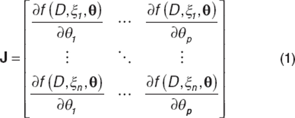The sensitivity of the system is defined by the Jacobian matrix (J), a n × p matrix of all first partial derivatives overall design points. D in the above expression represents the dose administered and f denotes the structural model.

Random noise in the observed response across the observation points is represented by the variance–covariance matrix (Σ);

Σ is a n × n square matrix and is computed from the product of the residual variance or random noise (σ²) and a n × n identity matrix (I_n). Equal variances across all observation points (σ₁² = σ₂² = … = σ_n²) are assumed. The assumption of equal variances can be relaxed without affecting the proposed identifiability method.

For a fixed-effects model, the M_F is constructed as

M_F in this instance represents the fixed-effects parameters and does not include the residual variance term.

The determinant is represented as .

Here, we propose a general and a revised criterion based on the |M_F| for the assessment of identifiability of models.

General criterion. Given a standard dose D, a specific design ξ, a parameter vector Θ, and a matrix showing an assumed random noise in the observed response Σ, the M_F of an identifiable model is invertible and its determinant is greater than zero. This general criterion is given as:

A singularity of the M_F with a determinant value of zero indicates that the model has one or more underlying parameters that are not identifiable. The M_F of a model that is not identifiable will be rank deficient and may contain a column and row of zeros. Although theoretically this criterion holds well, it may fall down on practical utility due to two reasons: (i) accuracy issues with matrix algebra operations can result in determinants for unidentifiable models to be represented as very small positive or negative values rather than zero and (ii) it requires a search across a large multidimensional design space to assess whether there exists a set of design variables that may satisfy the above criterion. In order to simplify the application of the criterion, we propose a second, revised criterion that is robust to the above shortfalls. It is based on the relation between the |M_F| and the random noise associated with the observed response.

Revised criterion: For all values of design variables (ξ), where n > p, and all design variables have a unique value (i.e., ξ_i ≠ ξ_j for all i ≠ j), the |M_F| approaches infinity as the associated noise approaches zero.

This criterion has greater practical utility than the general criterion as there are no limitations associated with its computation. As this criterion accounts for all designs, there is no necessity to search over the design space and an arbitrary set of values that fulfils the condition above in Eq. (5) can be chosen.

For fixed-effects models, the log of the determinant will be linearly related to the log of the random noise if the model is structurally identifiable. In the case of mixed-effects models, where M_F includes fixed-effects, random-effects, and the residual variance, we find

In the above expression, Ω is a vector of the variances of the random effects representing between the subject variability (BSV) in the population. V represents the first-order approximated likelihood of the variance. See Retout and Mentré for details relating to the expression for the population Fisher information matrix.²⁴ The asymptote of the log |M_F| in this case will not approach infinity. The numerical value to which Ψ asymptotes will have functional dependence on V. The relationship between the log of the determinant and the log of the random noise will be smooth and will asymptote to a constant Ψ in the space . We show this relationship graphically which for identifiable models shows the convergent nature, to the asymptote, of the relationship.

In the following sections, assessment of identifiability is based on the revised criterion across the models.

Results

Evaluation of the method for assessing identifiability of simple fixed-effects PK models

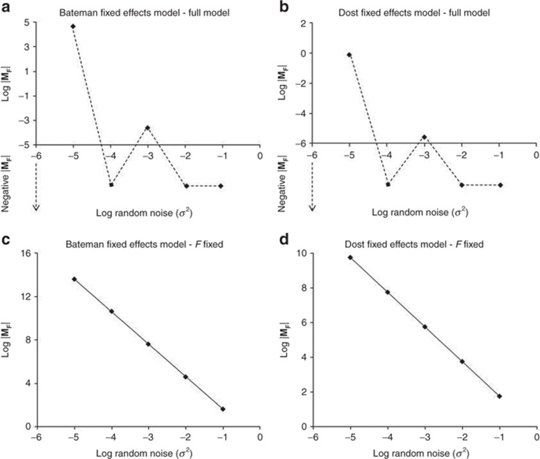
Assessment of the structural identifiability of the simple fixed-effects PK models indicated that both Bateman and Dost models were unidentifiable when all parameters (including F) were considered to be estimable. Both of these models were rendered identifiable by fixing F to a constant parameter value (Figure 1, see Supplementary Table S1 online). It is seen that unidentifiable models showed a discontinuous relationship for the log |M_F| vs. log random noise, whereas a continuous linear relationship was observed for identifiable models.

Figure 1.

Graphical representation of log |M_F| vs. log random noise (σ²) for simple fixed-effects pharmacokinetic models. In this graph, log |M_F| above the abscissa are as represented. Data below the abscissa represent the negative determinants that do not have log values and are shown for the purpose of displaying discontinuity of the line. (a,c) Bateman model, (b,d) Dost model; upper row: all parameters estimated, lower row: F fixed.

Identifying unidentifiable parameter(s) in the model: The results of the case deletion assessment for identifying the unidentifiable parameters in the Bateman fixed-effects model indicate that F is the unidentifiable parameter in the model (Supplementary Table S2 online).

Exploration of the method for testing the identifiability of random-effects parameters in simple population PK models

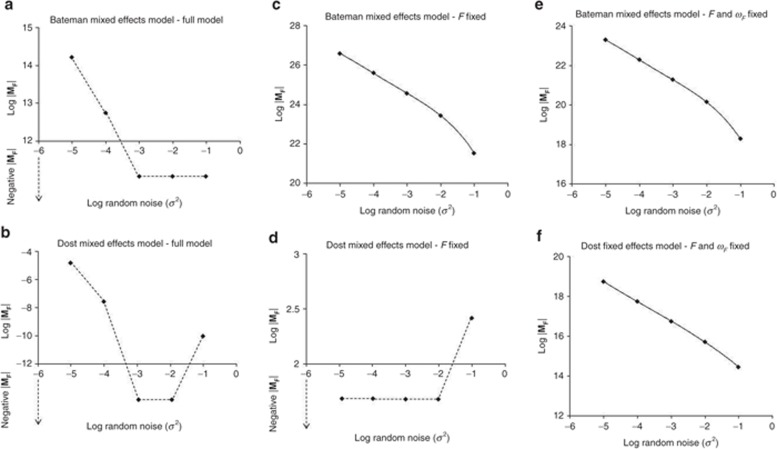
The criterion for assessment of identifiability of random-effects parameters was explored for the Bateman and Dost population PK models. The results for these mixed-effects models indicated that both the models were unidentifiable when all parameters were considered to be estimable. Fixing F alone rendered the Bateman model to become identifiable, whereas the Dost model was still unidentifiable. The Dost model was only identifiable when F and its BSV parameter ω_F were fixed (Figure 2, Supplementary Table S1 online).

Figure 2.

Graphical representation of log |M_F| vs. log random noise (σ²) for simple mixed-effects pharmacokinetic models. In this graph, log |M_F| above the abscissa are as represented. Data below the abscissa represent the negative determinants that do not have log values and are shown for the purpose of displaying discontinuity of the line. (a,c,e) Bateman model, (b,d,f) Dost model; left column: all parameters estimated, middle column: F fixed, right row: F and ω_F fixed.

Application of the method for identifiability analysis of a parent-metabolite PK model

Application of the criterion for assessment of identifiability of the motivating PK model was performed separately for models describing intravenous and oral administration. Both the models were considered for a fixed-effects analysis (as per the previous identifiability analysis reported by Evans et al.)⁶ and for a full mixed-effects analysis.

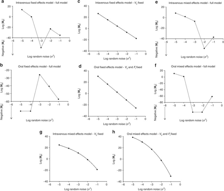
Assessment of the intravenous PK model: The intravenous fixed-effects model was unidentifiable when all parameters in the model were considered to be estimable. Fixing the value of V₃ (volume of distribution of metabolite in the central compartment) rendered the model structurally identifiable. The results of this analysis are in agreement with Evans et al.⁶ Results of the analysis of mixed-effects model revealed that all random-effects parameters were identifiable in the model. Although the fixed-effect parameter V₃ was unidentifiable, its corresponding random-effect parameter ω_V3 was identifiable (Figure 3, Supplementary Table S3 online). Note here that in the full mixed-effects model, the typical value of V₃ remained unidentifiable.

Figure 3.

Graphical representation of log |M_F| vs. log random noise (σ²) for parent-metabolite PK model of ivabradine. In this graph, log |M_F| above the abscissa are as represented. Data below the abscissa represent the negative determinants that do not have log values and are shown for the purpose of displaying discontinuity of the line. (a,c,e,g) Intravenous model, (b,d,f,h) oral model; (a,b): all parameters estimated (fixed-effects model), (c,d): V₃ ± F_I fixed (fixed-effects model), (e,f): all parameters estimated (mixed-effects model), (g,h): V₃ ± F_I fixed (mixed-effects model).

Assessment of the oral PK model: The oral fixed-effects model was unidentifiable when assessed with all parameters in the model. The model was still unidentifiable when v₃ was fixed. This was not unexpected as the model considered two additional parameters, namely, the fractions of parent and metabolite absorbed (F_I and F_S, respectively) following the oral administration of parent. Fixing one of these fractions (e.g., F_I) rendered the model identifiable, whereas F_S was identifiable as its corresponding volume term V₃ was already fixed in the model. Therefore, the oral fixed-effects model has two unidentifiable parameters. Assessment of the full mixed-effects model indicted that all of the random-effects parameters were identifiable. Random-effects parameters ω_V3 and ω_FI were still identifiable, although their corresponding fixed-effects parameters (V₃ and F_I, respectively) were unidentifiable (Figure 3, see Supplementary Table S3 online).

Discussion

Analysis of the results from both simple and a more complicated PK models have shown that the |M_F| shows a continuous linear log–log relationship with the associated random noise for structurally identifiable fixed-effects models. Similarly for structurally identifiable mixed-effects models, we also see a continuous relationship between log |M_F| and log residual variance, although the relationship is no longer linear on this scale due to the noninfinite asymptote.

An important feature of this analysis is that all identifiable models considered here yielded positive values of |M_F| for all values of the residual variance. This, however, is not in itself sufficient to confirm identifiability, as nonidentifiable models also yielded positive |M_F| values for some values of the residual variance. This emphasizes the need to show two necessary conditions for claiming identifiability for a model: (i) log |M_F| should have a continuous relationship with log residual variance and (ii) |M_F| should approach infinity (or a noninfinite asymptote for mixed-effects models) as residual variance approaches zero. The requirement to satisfy these two conditions requires|M_F| to be positive at varying random noise.

Evaluation of the results for the Bateman and Dost fixed- and mixed-effects models indicate that this method is capable of evaluating the structural identifiability of fixed- and random-effects parameters in population models. Analysis of the population models reveal that random-effects parameters may or may not follow the same rule as their corresponding fixed-effects parameters in regard to the identifiability. At this point, there does not appear to be a standard rule that could be applied to assess the identifiability of a random-effects parameter given known identifiability of a fixed-effects parameter. However, in the limited examples explored here, we see that in cases where the fixed-effects parameter is identifiable, the corresponding random-effects parameter is also always identifiable. However, other than for the Dost model, there appear to be circumstances when the random-effects parameters are identifiable despite the corresponding fixed-effects parameters being unidentifiable. This emphasizes the need to assess the identifiability of random-effects parameters in population models. Results from the assessment of the parent-metabolite PK model strengthen the ability of the current approach in assessing the identifiability of models with greater complexity and where identifiability may not be obvious. However, further investigations are needed to evaluate more precisely the identifiability of the random-effects parameters by assessing the M_F and to understand how they differ from their corresponding fixed-effects parameters in regard to identifiability.

Assessment of deterministic identifiability was not explicitly performed in this work. However, due to the known relationship between the information in a design and the standard error of the estimator (via Cramér-Rao inequality^25,26), it is straightforward from this analysis to choose a design that performs sufficiently well to meet the needs of deterministic identifiability. Once structural identifiability of the model is established, a formal assessment of the diagonal elements of the inverse of M_F can be made to assess the precision of parameter estimates for a candidate design at a value of residual variance of interest. It is noticed that highly constrained designs will impact the parameter estimation in the form of high SE values. These are consequences of deterministic identifiability issues that can be studied easily by the current approach before the study execution. Unlike other traditional available approaches for structural identifiability analysis that involve significant mathematical computation, our proposed approach is simple and any optimal design software (e.g., PFIM,²⁷ PopED,²⁸ and PopDes²⁹) can be used for assessing the identifiability of a model.

The proposed method, using an information theoretic approach, can be used to assess complete identifiability of population PK models. The criterion was able to evaluate the model in relation to indirectly assessing for a unique solution for individual parameters, a consequence of structural identifiability as shown in this study using simple and motivating PK models. The approach developed in this study can be used formally to assess the identifiability of proposed candidate models during study design. In the case of population models, the M_F can be studied separately, block wise to assess identifiability of the respective model parameters. The determinant of each submatrix can be studied to assess the identifiability of fixed effects, random effects, and error terms, respectively. We have not explored nonzero off-diagonal elements in the between subject variance–covariance matrix⁹; however, we believe that the techniques described here are likely to be generalizable to this and other circumstances. We also believe that the identifiability of random-effects parameters, such as the random effect on bioavailable fraction in the Bateman model, would be affected in presence of covariances (non-zero off diagonals), such as between clearance and volume of distribution, in the variance–covariance matrix, and further exploration is warranted.

In conclusion, we have developed an informal unified approach for the assessment of both structural and deterministic identifiability for both fixed- and random-effects parameters in population models. The approach was evaluated against both simple PK models with known identifiability issues and expanded to a more complicated parent-metabolite model. This approach is not limited to PK models and is extendable to identifiability analysis of population PKPD models.

Methods

Notation for nonlinear fixed- and mixed-effect models. We consider nonlinear models where the observed response is nonlinear in the parameter values. The notation for a nonlinear fixed-effects model is

y_j is the observed response at the j^th observation, and ε_j denotes the random error in the j^th observation. All other variables are defined as before, and we are using the same notation throughout the article.

Population models are encompassed within the framework of nonlinear mixed-effects models. Population models have two-stage hierarchy in describing the observed response across the individuals in a group of population.

Stage I constitutes the model for the data (structural model) representing the observed response in the population, which is given by

Here, y_ij represents j^th response in i^th individual.

Stage II constitutes the model for heterogeneity (covariate model) in the parameter values between individuals, which is given for any parameter Θ in the model by

Θ_i represents the parameter value in i^th individual (we have dropped the index specifying the parameter for simplicity but note that parameters may have covariance), g is the functional form of the covariate model, Z_i is a vector of covariates in i^th individual, is the population mean value of the parameter estimate, η_i is the random effect for the i^th individual, and ω is the variance of the random effect across the population. For the entire model, the BSV in all parameters with random effects is given by a q × q matrix ‘Ω', where q is the number of fixed-effect parameters that have a random effect (q ≤ p).

Diagonal elements represent the variances, and off-diagonal elements represent the covariances of the BSV.

Objective 1: Evaluation of the method for assessing identifiability of simple fixed-effects PK models. The criterion was explored by evaluating two simple PK models with known identifiability properties.

The first model considered was a one-compartment first-order input–output model (also known as “Bateman model”).^30,31 The model is given by:

The estimated parameters in the model are clearance (CL), volume of distribution (V), absorption rate constant (k_a), and bioavailable fraction (F), while k denotes the derived elimination rate constant.

The second model considered is the so-called “Dost model,”³² which is a simplification of the Bateman model.

The parameters in this model are similar to the parameters in the Bateman model, except k′ is a hybrid parameter that represents both the absorption and elimination rate constants (where k′ = k_a = k).

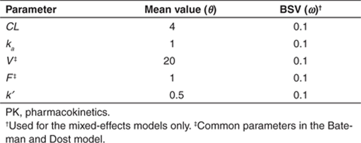
Identifiability analyses were performed using MATLAB 7.12 (version R2011a).³³ A constant dose of 100 mg and a generic study design for the sampling times (ξ = [0, 0.25, 0.5, 0.75, 1, 2, 4, 8, 12, 18, 24]^T) was assumed for both models. An arbitrary set of the parameter values was used (Table 1). The identifiability was assessed for both models based on two scenarios: (i) F was considered to be an unknown and estimable parameter and (ii) F was assumed to be known and fixed. Values for the random noise were log(σ²) = (−5, −4, −3, −2, and −1).

Table 1. Empirical set of parameter values used for the assessment of identifiability of simple PK models (fixed and mixed-effects models).

Identifying unidentifiable parameter(s) in the model. For unidentifiable models, the unidentifiable parameters were identified by a case deletion methodology. A specific column corresponding to a specific parameter was removed from the Jacobian matrix, and the subsequent effect on the determinant was evaluated. Cases (parameters) for which the deletion provided a linear relationship in log |M_F| vs. log random noise were taken as unidentifiable. The Bateman model was chosen as an illustrative example to show this method with two sets of parameterization (V, CL k_a, F and V, k_a, k, F).

Objective 2: Exploration of the method for testing identifiability of random-effects parameters in simple population PK models. The Bateman and Dost models were also used to explore the criterion for testing identifiability of random-effects parameters in a population analysis. The study design, dose, fixed-effects parameters and random noise in the observed response were the same as for Objective 1. The number of individuals in the population was set to 100. The parameter values, including the random-effects values, are presented in Table 1. Assessment of identifiability of the mixed-effects models was conducted using the POPT (Population OPTimal design) software tool,³⁴ a MATLAB application. Three scenarios were considered: (i) F and its corresponding random-effect BSV parameter ω_F were considered to be unknown and estimable parameters, (ii) F was assumed to be known and fixed, whereas ω_F was considered to be unknown and estimable, and (iii) F and ω_F were both assumed to be known and fixed.

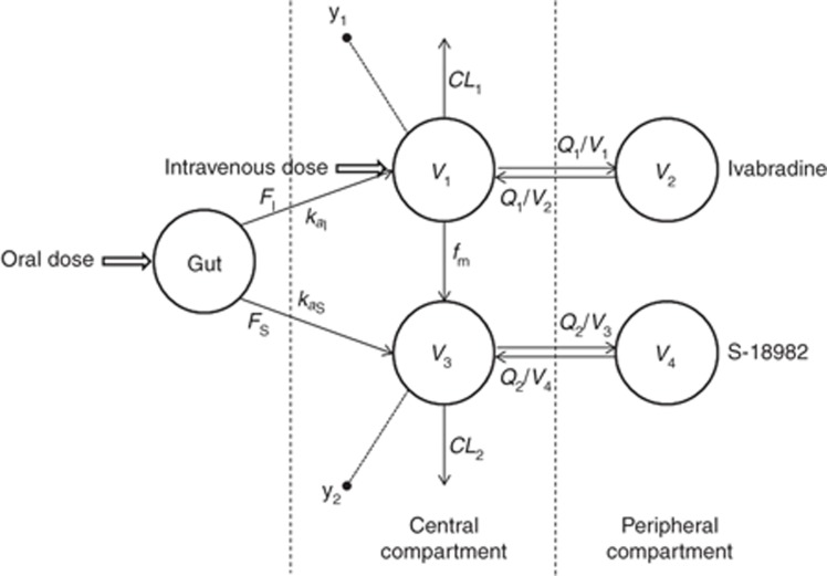
Objective 3: Application of the method for identifiability analysis of a parent-metabolite PK model. A combined parent-metabolite model describing the PK of ivabradine and its N-desmethylated metabolite (S-18982) was used as the motivating model (a schematic is provided in Figure 4). Ivabradine is a bradycardiac agent used in the treatment of angina pectoris and ischemic heart disorders. Probable identifiability issues associated with this model were first proposed by Duffull et al.³⁵ and a structural identifiability analysis based on a similarity transformation approach was reported by Evans et al.⁶ Ivabradine is administered either intravenously or as oral dose.

Figure 4.

Schematic representation of the combined parent-metabolite pharmacokinetic model of ivabradine. y₁ represents the observations corresponding to the parent (ivabradine) and y₂ represents the observations corresponding to the metabolite (S-18982).

In the case of intravenous administration, the drug is known to follow two-compartment pharmacokinetic behavior with first-order elimination. Metabolism of the parent produces S-18982, an active metabolite. The metabolite is also known to undergo two-compartment disposition similar to the parent.

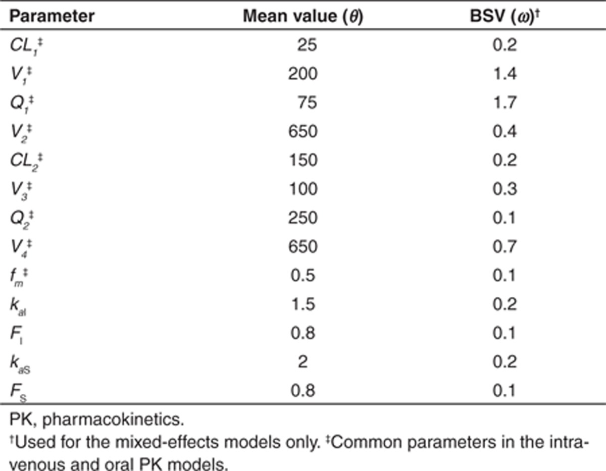
In the case of oral administration, a certain portion of the parent is known to undergo presystemic metabolism in the gut producing S-18982, which is then absorbed into the systemic circulation. There is also a possibility that a certain portion of the parent is neither absorbed into the systemic circulation nor undergoes presystemic metabolism. This portion of the parent can either convert into other, unknown metabolites, or may be eliminated from the gut. The parameters describing bioavailability for the parent and metabolite following oral administration of parent are denoted F_I and F_S, respectively. In the current study, identifiability analyses were performed separately for models describing intravenous and oral dose administration, each in two stages for fixed- and mixed-effects models, respectively, using POPT with an empirical set of parameter values (Table 2). All other study variables were similar as described for the simple example models. Algebraic equations used in the assessment of identifiability of intravenous and oral PK model are provided in the Supplementary Data online. The POPT code (p_model.m and popt_ini.m) of the oral mixed-effects PK model of ivabradine is available as Supplementary Data online.

Table 2. Empirical set of parameter values used for the assessment of identifiability of the fixed and mixed-effects parent-metabolite PK model for ivabradine.

Author contributions

V.S., J.K., I.G.T., and S.B.D.wrote the manuscript. V.S., J.K., I.G.T., and S.B.D. designed the research. V.S., J.K., I.G.T., and S.B.D. performed the research. V.S., J.K., I.G.T., and S.B.D. analyzed the data.

Conflict of interest

The authors declared no conflict of interest.

Study Highlights

References

- Haefner J.W. Modeling Biological Systems: Principles and Applications. Springer, New York; 2005. [Google Scholar]
- Cobelli C., Federspil G., Pacini G., Salvan A., Scandellari C. An integrated mathematical model of the dynamics of blood glucose and its hormonal control. Math. Biosci. 1982;58:27–60. [Google Scholar]
- Adam J.A. A simplified mathematical model of tumor growth. Math. Biosci. 1986;81:229–244. [Google Scholar]
- Wajima T., Isbister G.K., Duffull S.B. A comprehensive model for the humoral coagulation network in humans. Clin. Pharmacol. Ther. 2009;86:290–298. doi: 10.1038/clpt.2009.87. [DOI] [PubMed] [Google Scholar]
- Gibaldi M., Perrier D. Pharmacokinetics. M. Dekker, New York; 1975. [Google Scholar]
- Evans N.D., Godfrey K.R., Chapman M.J., Chappell M.J., Aarons L., Duffull S.B. An identifiability analysis of a parent-metabolite pharmacokinetic model for ivabradine. J. Pharmacokinet. Pharmacodyn. 2001;28:93–105. doi: 10.1023/a:1011521819898. [DOI] [PubMed] [Google Scholar]
- Bellman R., Åström K.J. On structural identifiability. Math. Biosci. 1970;7:329–339. [Google Scholar]
- Chappell M.J., Godfrey K.R., Vajda S. Global identifiability of the parameters of nonlinear systems with specified inputs: a comparison of methods. Math. Biosci. 1990;102:41–73. doi: 10.1016/0025-5564(90)90055-4. [DOI] [PubMed] [Google Scholar]
- Godfrey K.R., Chapman M.J., Vajda S. Identifiability and indistinguishability of nonlinear pharmacokinetic models. J. Pharmacokinet. Biopharm. 1994;22:229–251. doi: 10.1007/BF02353330. [DOI] [PubMed] [Google Scholar]
- Godfrey K.R., Jones R.P., Brown R.F. Identifiable pharmacokinetic models: the role of extra inputs and measurements. J. Pharmacokinet. Biopharm. 1980;8:633–648. doi: 10.1007/BF01060058. [DOI] [PubMed] [Google Scholar]
- Jacquez J.A. Identifiability: the first step in parameter estimation. Fed. Proc. 1987;46:2477–2480. [PubMed] [Google Scholar]
- Jacquez J.A., Perry T. Parameter estimation: local identifiability of parameters. Am. J. Physiol. 1990;258:E727–E736. doi: 10.1152/ajpendo.1990.258.4.E727. [DOI] [PubMed] [Google Scholar]
- Cobelli C., DiStefano J.J., 3rd Parameter and structural identifiability concepts and ambiguities: a critical review and analysis. Am. J. Physiol. 1980;239:R7–24. doi: 10.1152/ajpregu.1980.239.1.R7. [DOI] [PubMed] [Google Scholar]
- Yates J.W., Jones R.D., Walker M., Cheung S.Y. Structural identifiability and indistinguishability of compartmental models. Expert Opin. Drug Metab. Toxicol. 2009;5:295–302. doi: 10.1517/17425250902773426. [DOI] [PubMed] [Google Scholar]
- Bortz D.M., Nelson P.W. Model selection and mixed-effects modeling of HIV infection dynamics. Bull. Math. Biol. 2006;68:2005–2025. doi: 10.1007/s11538-006-9084-x. [DOI] [PubMed] [Google Scholar]
- Duffull S.B., Wright D.F., Winter H.R. Interpreting population pharmacokinetic-pharmacodynamic analyses - a clinical viewpoint. Br. J. Clin. Pharmacol. 2011;71:807–814. doi: 10.1111/j.1365-2125.2010.03891.x. [DOI] [PMC free article] [PubMed] [Google Scholar]
- Knutsson I.-S.N., Aarons L. 12th Annual Scientific Meeting, Population Approach Group in Australia and New Zealand. Adelaide, Australia; 2010. Identifiability of random effects parameters in mixed effects models. [Google Scholar]
- Guedj J., Thiébaut R., Commenges D. Practical identifiability of HIV dynamics models. Bull. Math. Biol. 2007;69:2493–2513. doi: 10.1007/s11538-007-9228-7. [DOI] [PubMed] [Google Scholar]
- Bonate P.L. The Art of Modeling. Springer US, Boston, MA; 2011. pp. 1–60. [Google Scholar]
- Bellu G., Saccomani M.P., Audoly S., D'Angiò L. DAISY: a new software tool to test global identifiability of biological and physiological systems. Comput. Methods Programs Biomed. 2007;88:52–61. doi: 10.1016/j.cmpb.2007.07.002. [DOI] [PMC free article] [PubMed] [Google Scholar]
- Chis O., Banga J.R., Balsa-Canto E. GenSSI: a software toolbox for structural identifiability analysis of biological models. Bioinformatics. 2011;27:2610–2611. doi: 10.1093/bioinformatics/btr431. [DOI] [PMC free article] [PubMed] [Google Scholar]
- Mentré F., Mallet A., Baccar D. Optimal design in random-effects regression models. Biometrika. 1997;84:429–442. [Google Scholar]
- Fedorov V.V., Leonov S.L. Optimal design of dose response experiments: a model-oriented approach. Drug. Inf. J. 2001;35:1373–1383. [Google Scholar]
- Retout S., Mentré F. Further developments of the Fisher information matrix in nonlinear mixed effects models with evaluation in population pharmacokinetics. J. Biopharm. Stat. 2003;13:209–227. doi: 10.1081/BIP-120019267. [DOI] [PubMed] [Google Scholar]
- Cramer H. Mathematical Methods of Statistics. Princeton University Press, Princeton, USA; 1946. [Google Scholar]
- Rao C.R. Information and the accuracy attainable in the estimation of statistical parameters. Bull. Calcutta Math. Soc. 1945;37:81–91. [Google Scholar]
- Bazzoli C., Retout S., Mentré F. Design evaluation and optimisation in multiple response nonlinear mixed effect models: PFIM 3.0. Comput. Methods Programs Biomed. 2010;98:55–65. doi: 10.1016/j.cmpb.2009.09.012. [DOI] [PubMed] [Google Scholar]
- Nyberg J., Ueckert S., Strömberg E.A., Hennig S., Karlsson M.O., Hooker A.C. PopED: an extended, parallelized, nonlinear mixed effects models optimal design tool. Comput. Methods Programs Biomed. 2012;108:789–805. doi: 10.1016/j.cmpb.2012.05.005. [DOI] [PubMed] [Google Scholar]
- Gueorguieva I., Ogungbenro K., Graham G., Glatt S., Aarons L. A program for individual and population optimal design for univariate and multivariate response pharmacokinetic-pharmacodynamic models. Comput. Methods Programs Biomed. 2007;86:51–61. doi: 10.1016/j.cmpb.2007.01.004. [DOI] [PubMed] [Google Scholar]
- Bateman H. Solution of a system of differential equations occurring in the theory of radioactive transformations. Proc. Camb. Philol. Soc. 1910;15:423–427. [Google Scholar]
- Garrett E.R. The Bateman function revisited: a critical reevaluation of the quantitative expressions to characterize concentrations in the one compartment body model as a function of time with first-order invasion and first-order elimination. J. Pharmacokinet. Biopharm. 1994;22:103–128. doi: 10.1007/BF02353538. [DOI] [PubMed] [Google Scholar]
- Dost F.H. Grundlagen der Pharmakokinetik. G. Thieme, Stuttgart: 2. Gufl. 1968;2:38–47. [Google Scholar]
- The MathWorks Inc. Getting Started with MATLAB®, Technical Computing Manual . < http://www.mathworks.com > ( The MathWorks Inc., MA, USA; 2006 [Google Scholar]
- Duffull S.B., Denman N., Kimko H., Eccleston J.Population OPTimal design. POPT - Installation and User Guide . < http://www.winpopt.com > ( Duffull, S.B., School of Pharmacy, University of Otago, Dunedin, New Zealand; 2012 [Google Scholar]
- Duffull S.B., Chabaud S., Nony P., Laveille C., Girard P., Aarons L. A pharmacokinetic simulation model for ivabradine in healthy volunteers. Eur. J. Pharm. Sci. 2000;10:285–294. doi: 10.1016/s0928-0987(00)00086-5. [DOI] [PubMed] [Google Scholar]
Associated Data
This section collects any data citations, data availability statements, or supplementary materials included in this article.