The Association Between Racial Disparity in Income and Reported Sexually Transmitted Infections

Abstract

Objectives. We examined the association between racial disparity in income and reported race-specific county-level bacterial sexually transmitted infections (STIs) in the United States focusing on disparities between Blacks and Whites.

Methods. Data are from the US 2000 decennial census. We defined 2 race–income county groups (high and low race–income disparity) on the basis of the difference between Black and White median household incomes. We used 2 approaches to examine disparities in STI rates across the groups. In the first approach, we computed and compared race-specific STI rates for the groups. In the second approach, we used spatial regression analyses to control for potential confounders.

Results. Consistent with the STI literature, chlamydia, gonorrhea, and syphilis rates for Blacks were substantially higher than were those for Whites. We also found that racial disparities in income were associated with racial disparities in chlamydia and gonorrhea rates and, to a lesser degree, syphilis rates.

Conclusions. Racial disparities in household income may be a more important determinant of racial disparities in reported STI morbidity than are absolute levels of household income.

Racial disparities in sexually transmitted infections (STIs) in the United States have been documented extensively.^1,2 In fact, racial disparities in STIs and HIV are ranked among the greatest racial disparities in health in the United States.³ For example, in 2009 the rates of chlamydia and syphilis among Blacks in the United States were more than 8-fold the rates among Whites, and the disparity was even more pronounced for gonorrhea (20-fold).¹ Effective STI control and prevention efforts should include strategies to reduce racial disparities,² which was one of the major objectives of Healthy People 2010.³ However, owing to the failure to meet the Healthy People 2010 goals, reducing or eliminating health disparity is one of the overarching goals of Healthy People 2020.⁴ Thus, examining the factors that cause (or are associated with) racial disparities in STI rates can inform strategies to reduce or eliminate these disparities.

When examining the aspects of social structure associated with endemically high rates of gonorrhea at the county level, Thomas and Gaffield⁵ found a positive association between gonorrhea rates and income dualism (i.e., the average income differences between Black and White families) after controlling for other county-level demographic characteristics. Thomas and Gaffield suggest that if other studies confirm this association, efforts to reduce the substantial racial disparities in gonorrhea rates should include strategies to improve the existing income inequalities between Blacks and Whites as well.

We examined the association between county-level racial disparity in income and reported bacterial STI rates. Our analysis adds to Thomas and Gaffield’s novel study⁵ in 2 main ways. First, we investigated county-level racial disparity in income and 3 reportable STIs (total rates and specific rates for race and gender of chlamydia, gonorrhea, and primary and secondary syphilis) using more recent data (2000) on all the counties in the 48 contiguous states, whereas Thomas and Gaffield focused on county-level gonorrhea rates in 14 Southern states using data from 1986 to 1995. Second, we used spatial regression analyses to control for spatial dependence in reported STIs across counties; “spatial dependence” refers to the fact that STI rates in a given county are usually correlated with STI rates in bordering counties.

Thus, our key contribution to the literature is to augment the work of Thomas and Gaffield by providing a comprehensive, updated analysis of county-level racial disparities in income and reported STIs (total rates and specific rates by race and gender). Studying the association of racial disparities in income with STI disparities by race can promote further examination of the mechanisms through which race–income disparities may be associated with or exacerbate disparities in STI rates between Blacks (or other racial minorities) and Whites in the United States. In addition, these studies may provide some insights into income distribution between racial groups as it relates to STI disparities and can inform decisions and strategies aimed at reducing or eliminating these disparities.

METHODS

We obtained race-specific county-level median household income data from the US 2000 decennial census. We then created a continuous variable (race–income disparity measure) as the difference between the median household income for Whites and the median household income for Blacks. Next, we defined 2 race–income county groups (high race–income disparity and low race–income disparity) on the basis of Black median household income and White median household income at the county level for all the counties in the 48 contiguous states in the United States. We used the median household income as the population-level measure of household income because outliers do not influence it. Of the 3107 counties in the 48 contiguous states eligible for our analysis, we excluded 383 (12.3%) from our analysis because either no Blacks resided in the counties or median household income data were missing.

We defined the high race–income disparity group as comprising those counties in which Black median household income was lower than the national average (i.e., $41 994⁶) and White median household income was above the national average. For the high race–income disparity group, the median household income was $46 046 for Whites and $29 919 for Blacks. The average difference between the median White household income and Black household income was $17 775 (n = 479). We defined the low race–income disparity group as comprising the remaining 2245 counties. For the low race–income disparity group, the median household income was $34 551 for Whites and $23 380 for Blacks, and the median of the difference in household income was $11 282.

Figure 1 shows the spatial distribution of the counties that make up each of the groups we have described. On the basis of rural–urban continuum codes,⁷ more than 80% (390/479) of the high race–income disparity counties were metropolitan counties (i.e., counties assigned rural–urban continuum codes 1–3⁷). However, approximately 30% of the low race–income disparity counties were metropolitan counties.

FIGURE 1—

County map of the 48 contiguous states showing the counties that constituted the race–income groups.

Next, we used 2 approaches to examine disparities in reported STI rates between the 2 race–income groups we have described (high race–income disparity vs low race–income disparity). In the first approach, we computed and compared race-specific STI rates for the 2 groups. In the second approach, we used regression analysis to control for county-level characteristics and spatial dependence (or spatial clustering).

Calculation of Infection Rates in the 2 County Groups

We obtained county-level race-specific morbidity data for chlamydia, gonorrhea, and primary and secondary syphilis from the National Electronic Telecommunications System for Surveillance for 1999–2001. For each of the 2 groups, we calculated temporally smoothed STI rates^8,9 (i.e., reported cases per 100 000 residents) using the total number of cases and population size for all 3 years as follows for Black (both genders), White (both genders), male (both races), female (both races), and total (both genders and races): (sum of cases for 1999, 2000, and 2001/sum of the population for 1999, 2000, and 2001) × 100 000.

Regression Analysis of County-Level Infection Rates

To explore reported STI rates across the high and low race–income disparity groups in more detail, we used spatial regression techniques that accounted for spatial dependence and controlled for county characteristics. We used 2 measures of income disparity in the regression analyses. First, we used the dichotomous measure we have described in which we classified counties as high race-income disparity or low race–income disparity. Second, we used a continuous measure of race-income disparity, which we calculated as the difference between White median household income and Black median household income. Specifically, we used 2 regression models for each STI. In model 1, we included the high race–income disparity group as a dichotomous explanatory variable in the regression analyses (1 if the county belonged to the high race–income disparity group, 0 otherwise). In model 2, we included both the continuous measure of race-income disparity and the log of median household income as continuous variables in place of the dichotomous variable for the high race–income disparity group. The dependent variables were the rates of each STI (i.e., Black [both genders], White [both genders], male [both races], female [both races], and total [both genders and races]). Thus, there were 10 sets of regression results for each STI (2 models, both of which we estimated using the 5 dependent variables).

We included control variables for demographic and socioeconomic factors as suggested by previous studies, using data from the US 2000 decennial census.^8–12 These county-level control variables included percentage Black, percentage White (referent race category), percentage Hispanic, percentage American Indian, percentage American Asian, percentage aged 18 to 24 years, percentage aged 25 to 44 years, log of male–female population ratio, log of population density, log of birth rate, log of death rate, log of crime rate (i.e., violent and property), and a suburban commute index (i.e., percentage commuting from other counties). Because the primary variables of interest were derived from median household incomes, we excluded control variables that were strongly correlated with median household income such as percentage below poverty line, percentage owner-occupied housing, and per capita income in models 1 and 2. However, median household income was included in model 2 because we determined that it was not correlated with the race–income disparity measure (correlation coefficient = 0.04; P = .21).

Technical Details of Regression Analysis

Following methodology used in previously published studies,^8,9 we used a spatial error model to account for spatial dependence (or spatial clustering). To account for variations in county-level rates in and across states, we used a state-specific fixed-effects model for each STI (i.e., chlamydia, gonorrhea, and primary and secondary syphilis). Because there were zero cases in some counties (especially for primary and secondary syphilis) and for the benefit of uniformity in result interpretation, we added 1 to the computed rates and converted the resulting number into the natural logarithm.¹³

We scaled the coefficients of the race–income disparity variable (a continuous variable) to reflect the approximate percentage change in STI rates associated with each $10 000 increase in the difference between White and Black median incomes. We transformed the coefficients of the high race–income disparity group variable (a dichotomous variable) as (exp^coefficient − 1) × 100 and interpreted them as the percentage difference in STI rates for counties in the high race–income disparity group compared with counties in the low race–income disparity group on average (the omitted group).

To account for differences in rural–urban county rates, we included the 2003 rural–urban continuum codes the US Department of Agriculture, Economic Research Services⁷ developed as dichotomous variables. We included regional dichotomous variables for preliminary analyses, but we dropped them for the state-specific fixed-effect model estimation because of high multicollinearity.

We checked for multicollinearity by computing the variance inflation factors using 10 as the cutoff point.¹⁴ We computed bootstrapped standard errors for coefficients from 50 replications. We used ArcGIS, version 9.3 (ESRI, Redland, CA) to obtain the polygons representing all the counties in the United States. We used GeoDa, version 0.9.5-I¹⁵ to create spatial lag variables and to perform preliminary spatial regression analyses. We used SAS, version 9.2 (SAS Institute, Cary, NC) and Stata, version 11.1 (StataCorp LP, College Station, TX) for result validation and regression diagnostics.

RESULTS

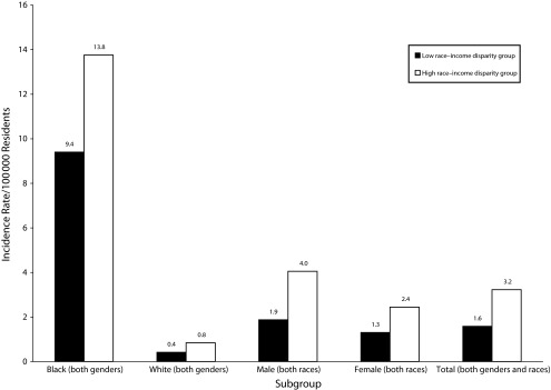
Reported STI rates (number of cases per 100 000 residents) for the 2 groups (i.e., high and low race–income disparity) by race and gender are presented in Figures 2, 3, and 4. For both groups, the STI rates for Blacks were at least 4 times higher than were those for Whites. Chlamydia rates were at least 2 times higher in women than in men in both groups. However, Black men had higher gonorrhea and syphilis rates than did Black women, whereas White men had higher syphilis rates than did White women (data not shown). Finally, almost all the STI rates were higher in the high race–income disparity group than were those in the low race–income disparity group, as depicted in the 3 figures. Chlamydia in White women was the only exception in which the incidence rate in the low race–income disparity group was higher than was the incidence rate among the high race–income disparity group (data not shown).

FIGURE 2—

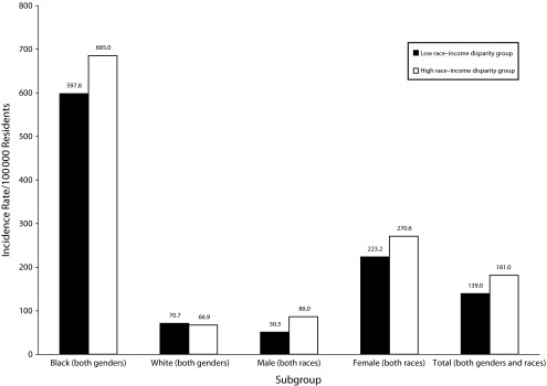
Chlamydia incidence rates (per 100 000 residents) for high and low race–income disparity groups by race and gender: United States, 1999–2001.

Note. Because the computed rates were for the entire population for each group, we did not perform significance tests.

FIGURE 3—

Gonorrhea incidence rates (per 100 000 residents) for high and low race–income disparity groups by race and gender: United States, 1999–2001.

Note. Because the computed rates were for the entire population for each group, we did not perform significance tests.

FIGURE 4—

Primary and secondary syphilis incidence rates (per 100 000 residents) for high and low race–income disparity groups by race and gender: United States, 1999–2001.

Note. Because the computed rates were for the entire population for each group, we did not perform significance tests.

Regression Analysis Results of County-Level Infection Rates

Table 1 summarizes the regression results. Because of the large number of regression analyses we conducted (a total of 30), we showed the results for the 2 independent variables of interest (i.e., high race–income disparity groups in model 1 and race–income disparity in model 2) for each of the 3 diseases we examined. Additionally, for ease of interpretation, we converted the results into percentages using the methods we have described. For example, the 16 in the first row of the third column of results indicates that male chlamydia rates were about 16% higher in the high race–income disparity counties than were those in the low race–income disparity counties on average. Furthermore, the 4 in the second row of the third column of results indicates that each $10 000 increase in race–income disparity (the difference between median household income for Whites and Blacks) was associated with a 4% increase in men’s chlamydia rates on average. We have provided more information on the 6 major regression results (2 models for each STI) in which the dependent variables were the total STI rates (data available as a supplement to the online version of this article at http://www.ajph.org). Detailed results from the race- and gender-specific regression analyses are available from the lead author on request.

TABLE 1—

Results of the Spatial Regression Analyses of the Transformed Chlamydia, Gonorrhea, and Primary and Secondary Syphilis Rates (n = 2724 Counties): United States, 2000

Variable	Black, %	White, %	Male, %	Female, %	Total, %
Chlamydia
Model 1a: High race–income disparity group	34**	−3	16**	8*	9*
Model 2b: race–income disparity (continuous)	13**	2*	4*	4**	4**
Gonorrhea
Model 1a: High race–income disparity group	28**	6	24**	17**	23**
Model 2b: race–income disparity (continuous)	11**	3*	5**	5**	5**
Primary and secondary syphilis
Model 1a: High race–income disparity group	12*	1	3	3	2
Model 2b: race–income disparity (continuous)	1	0	4	5	2

Note. Each model included all the control variables. More detailed information on the results for the control variables for each disease model using total rates as the dependent variable can be found in a supplement to the online version of this article at http://www.ajph.org.

^aResults for model 1 are interpreted as the percentage difference in the dependent variable between the high vs low race–income disparity counties on average.

^bResults for model 2 are interpreted as the change in the dependent variable associated with a $10 000 increase in the difference between White and Black median incomes on average.

*P < .05; **P < .01.

In model 1, high race–income disparity counties had significantly higher rates of chlamydia and gonorrhea than did low race–income disparity counties on average after controlling for other socioeconomic factors. The 1 exception was chlamydia rates in Whites, for which we did not observe any significant difference for high race–income disparity counties versus low race–income disparity counties. In model 2, in which race–income disparity was the independent variable of interest, chlamydia and gonorrhea rates were significantly and positively associated with the degree of income inequality.

We did not detect any significant associations between syphilis rates and race–income disparities, with 1 exception. In model 1, syphilis rates in Blacks were 12% higher (P < .05) in high race–income disparity counties than were those in low race–income disparity counties on average. The coefficients for other independent variables are not included in Table 1 but are available as a supplement to the online version of this article (http://www.ajph.org) for selected regressions for the 6 main regression analyses. The coefficients of the other independent variables were generally consistent with those in the existing literature. For example, for chlamydia and gonorrhea, the percentage aged 18 to 24 years was associated with higher STI rates (P < .01) than were all other age groups, consistent with the higher reported chlamydia and gonorrhea rates among adolescents and young adults relative to other age groups.¹ Furthermore, percentage Black and percentage American Indians were associated with higher STI rates for all 3 STIs (P < .05) than was percentage White, consistent with reported patterns. The coefficient of the ratio of the male–female population was consistently negative, implying that higher incidence of reported STIs were associated with counties with a lower male–female population ratio.

Technical Details of Regression Analysis

Our check for multicollinearity was in the recommended limit of 10; the highest variance inflation factor was 4.8 (mean = 2.3) for all the regression analyses. The error spatial lag was also significant (P < .01) for each disease model, implying that spatial dependence was fairly accounted for in the regression.^15,16 The variations in the independent variables included in the analyses explained at least 50% of the variations in the transformed total incidence rates for all 3 diseases, as the overall R²s indicate (data available as a supplement to the online version of this article at http://www.ajph.org). Additionally, the signs of the coefficients were consistent with previous studies.^8–12

DISCUSSION

We used 2 approaches to examine the association between county-level racial disparity in income and reportable bacterial STIs (total rates and specific rates by race and gender) using US 2000 decennial census data for all the counties in the 48 contiguous states in the United States, focusing on rates of the 3 common bacterial STIs (i.e., chlamydia, gonorrhea, and primary and secondary syphilis) among Blacks and Whites. In both approaches, we found that STI rates for Blacks were substantially higher than were STI rates for Whites. These results are consistent with findings from previous studies.^2,17–20 Additionally, we found that counties with greater racial disparities in income typically had higher STI rates than did counties with smaller racial disparities in income. These findings provide evidence of an association between racial disparity in income and racial disparities in STI rates at the county level and are consistent with findings from a previous study that found similar results for gonorrhea rates in 14 Southern states using earlier incidence data (1986–1995).⁵ Our results also imply that these associations persist at the county level in the year 2000 and extend to the national level.

Higher STI rates in the high race–income disparity group than in the low race–income disparity group cannot be explained by differences in overall (i.e., Black and White) income. Median household income for Blacks was about $23 000 in the low-income disparity counties and about $30 000 in the high-income disparity counties. If absolute levels of income (rather than income disparity) were the main determinant of STI morbidity, STI rates in Blacks would be expected to be lower in the high race–income disparity group than in the low race–income disparity group. The same was true for Whites: White STI rates in the low-income disparity counties (with a White median income of approximately $35 000) were lower than were White STI rates in the high-income disparity counties (with a White median income of approximately $46 000). Thus, race–income disparities were associated with higher STI rates for both races, although the degree of association was higher for Blacks than for Whites.

Several hypotheses have been suggested to explain differences between Black and White STI rates.²¹ Differential STI prevalence in racial subgroups combined with race-assortative sexual mixing (or sexual segregation) is perhaps the most powerful of these explanations.^5,22–24 Disparity in income across races is correlated with race-based residential segregation, which in turn could contribute to sexual segregation.⁵ Accordingly, it is conceivable that high levels of race–income disparity exacerbate race-based sexual segregation, thereby increasing racial difference in STI rates; whereas low levels of race–income disparity may have a damping effect on race-based sexual segregation. Another way that White–Black income disparity might contribute to higher STI rates would be if decisions regarding allocation of public STI prevention and treatment resources were made predominantly by Whites without awareness of or sensitivity to the issues of care provision to Blacks.⁵

More than 80% of the high race–income disparity counties were classified as metropolitan counties. Thus, an important potential confounding factor is that urban areas might be more likely than are nonurban areas to have racial disparities in income and to have sizeable populations of men who have sex with men (MSM).^25–27 However, because of lack of data on sexual orientation–specific rates at the county level, we were not able to control for this confounding factor. As a result, different STI dynamics in urban versus nonurban areas unrelated to income disparity (e.g., higher rates of STIs in urban MSM than in men overall) might contribute to the higher gonorrhea and primary and secondary syphilis rates we observed for the high versus low race–income disparity group in the first approach.

Additionally, the higher total gonorrhea and primary and secondary syphilis rates we found are mainly because of higher rates in men, suggesting that STIs in MSM may indeed have contributed to the disparities we observed in the first approach. However, it is unlikely that our results can be explained as an artifact of MSM in urban areas. This is because gonorrhea and primary and secondary syphilis rates in Black women are higher in the high race–income disparity group than in the low race–income disparity group, and MSM might not be expected to have this degree of impact on gonorrhea and syphilis rates in women.

This study is subject to several limitations, including the usual limitations associated with STI surveillance data.¹ Some cases were assigned to missing or unknown counties. We assembled the data from reported cases of infection that come from different sources with different testing and reporting practices. As a result, there may be varying levels of underreporting for some jurisdictions, and the degree of underreporting might vary by race. Owing to the comparatively high asymptomatic nature of chlamydia,²⁸ reported chlamydia rates may be more of an artifact of the existing screening patterns than of actual incidence rates.¹

Our choice of the national median household income as a cutoff in categorizing high versus low race–income disparity counties was arbitrary. However, our inclusion of the difference between White and Black median household income confirmed the robustness of our results. Because our findings are derived from population-level analyses, limitations associated with ecological analyses are applicable. Finally, we did not account for spatial heterogeneity (i.e., we did not allow parameter coefficients to vary by region^16,29) in our spatial regression analyses. However, our use of a state-specific fixed-effect estimation procedure, to some extent, reduced the impact of this limitation on our results.

Our race–income categorization adds several new insights to the existing literature regarding income, race, and reported STI rates. Most importantly, the grouping of counties that we developed allowed us to examine not only the association between STI rates and income but also the association between racial disparities in STI rates and racial disparities in income. Our findings show the need for further examination of the mechanisms through which race–income disparity may be associated with or exacerbate disparities in STI rates.

Future research is needed to quantify disparities in income more specifically and to explore alternate methods and cutoffs (such as different multiples of poverty) for examining the association between race–income disparities and disparities in other health outcomes as well as to use more recent data as they become available to examine trends in these associations.

References

- 1.Centers for Disease Control and Prevention Sexually Transmitted Disease Surveillance, 2009. Atlanta, GA: US Department of Health and Human Services; 2010 [Google Scholar]
- 2.Newman LM, Berman SM. Epidemiology of STD disparities in African American communities. Sex Transm Dis. 2008;35(12, suppl):S4–S12 [DOI] [PubMed] [Google Scholar]
- 3.Keppel KG. Ten largest racial and ethnic health disparities in the United States based on Healthy People 2010 objectives. Am J Epidemiol. 2007;166(1):97–103 [DOI] [PubMed] [Google Scholar]
- 4.US Department of Health and Human Services Healthy People 2020 Framework: The Vision, Mission and Goals of Healthy People 2020. Washington, DC: Office of Disease Prevention and Health Promotion; 2012 [Google Scholar]
- 5.Thomas JC, Gaffield ME. Social structure, race, and gonorrhea rates in the southeastern United States. Ethn Dis. 2003;13(3):362–368 [PubMed] [Google Scholar]
- 6.US Census Bureau Profile of Selected Economic Characteristics: 2000. Washington, DC; 2000 [Google Scholar]
- 7.US Department of Agriculture Rural Urban Continuum. Washington, DC: Economic Research Services; 2008 [Google Scholar]
- 8.Owusu-Edusei K, Jr, Chesson HW. Using spatial regression methods to examine the association between county-level racial/ethnic composition and reported cases of chlamydia and gonorrhea: an illustration with data from the state of Texas. Sex Transm Dis. 2009;36(10):657–664 [DOI] [PubMed] [Google Scholar]
- 9.Owusu-Edusei K, Jr, Doshi SR. County-level sexually transmitted disease detection and control in Texas: do sexually transmitted diseases and family planning clinics matter? Sex Transm Dis. 2011;38(10):970–975 [DOI] [PubMed] [Google Scholar]
- 10.Semaan S, Sternberg M, Zaidi A, Aral SO. Social capital and rates of gonorrhea and syphilis in the United States: spatial regression analyses of state-level associations. Soc Sci Med. 2007;64(11):2324–2341 [DOI] [PubMed] [Google Scholar]
- 11.Chesson H, Owusu-Edusei K., Jr Examining the impact of federally-funded syphilis elimination activities in the USA. Soc Sci Med. 2008;67(12):2059–2062 [DOI] [PubMed] [Google Scholar]
- 12.Kilmarx PH, Zaidi AA, Thomas JCet al. Sociodemographic factors and the variation in syphilis rates among US counties, 1984 through 1993: an ecological analysis. Am J Public Health. 1997;87(12):1937–1943 [DOI] [PMC free article] [PubMed] [Google Scholar]
- 13.van Belle G, Fisher LD, Heagerty PJ, Lumley TS. Biostatistics: A Methodology for the Health Sciences. New York, NY: John Wiley & Sons; 2004 [Google Scholar]
- 14.Belsley DA, Kuh E, Welsch RE. Regression Diagnostics. New York, NY: John Wiley & Sons; 1980 [Google Scholar]
- 15.Anselin L, Syabri I, Kho Y. GeoDa: an introduction to spatial data analysis. Geogr Anal. 2006;38(1):5–22 [Google Scholar]
- 16.LeSage JP. Econometric Toolbox. Available at: www.spatial-econometrics.com. Accessed December 15, 2011. [Google Scholar]
- 17.Adimora AA, Schoenbach VJ. Social context, sexual networks, and racial disparities in rates of sexually transmitted infections. J Infect Dis. 2005;191(suppl 1):S115–S122 [DOI] [PubMed] [Google Scholar]
- 18.Aral SO. Understanding racial–ethnic and societal differentials in STI. Sex Transm Infect. 2002;78(1):2–4 [DOI] [PMC free article] [PubMed] [Google Scholar]
- 19.Aral SO. Social and behavioral determinants of sexually transmitted disease: scientific and technologic advances, demography, and the global political economy. Sex Transm Dis. 2006;33(12):698–702 [DOI] [PubMed] [Google Scholar]
- 20.Ellen JM, Kohn RP, Bolan GA, Shiboski S, Krieger N. Socioeconomic differences in sexually transmitted disease rates among Black and White adolescents, San Francisco, 1990 to 1992. Am J Public Health. 1995;85(11):1546–1548 [DOI] [PMC free article] [PubMed] [Google Scholar]
- 21.Kraut-Becher J, Eisenberg M, Aral SO. Racial and ethnic disparities in HIV infection in the United States. Focus. 2009;24(2):1–8 [Google Scholar]
- 22.Hallfors DD, Iritani BJ, Miller WC, Bauer DJ. Sexual and drug behavior patterns and HIV and STD racial disparities: the need for new directions. Am J Public Health. 2007;97(1):125–132 [DOI] [PMC free article] [PubMed] [Google Scholar]
- 23.Laumann EO, Youm Y. Racial/ethnic group differences in the prevalence of sexually transmitted diseases in the United States: a network explanation. Sex Transm Dis. 1999;26(5):250–261 [DOI] [PubMed] [Google Scholar]
- 24.Aral SO. Sexual network patterns as determinants of STD rates: paradigm shift in the behavioral epidemiology of STDs made visible. Sex Transm Dis. 1999;26(5):262–264 [DOI] [PubMed] [Google Scholar]
- 25.Catania JA, Osmond D, Stall RDet al. The continuing HIV epidemic among men who have sex with men. Am J Public Health. 2001;91(6):907–914 [DOI] [PMC free article] [PubMed] [Google Scholar]
- 26.Peterman TA, Heffelfinger JD, Swint EB, Groseclose SL. The changing epidemiology of syphilis. Sex Transm Dis. 2005;32(10 suppl):S4–S10 [DOI] [PubMed] [Google Scholar]
- 27.Squires GD, Kubrin CE. Privileged places: race, uneven development and the geography of opportunity in urban America. Urban Stud. 2005;42(1):47–68 [Google Scholar]
- 28.Stamm WE. Chlamydia trachomatis infections in the adult. : Holmes KK, Sparling PF, Stamm WEet al. Sexually Transmitted Diseases. New York, NY: McGraw Hill; 2008:575–593 [Google Scholar]
- 29.Anselin L, Bera S. Spatial dependence in linear regression models with an introduction to spatial econometrics. : Ullah A, Giles DA, Handbook of Applied Economic Statistics. New York, NY: Marcel Dekker; 1998: 237–289 [Google Scholar]