

Abstract
We show that, in the presence of uncontrolled environmental confounding, joint tests for the presence of a main genetic effect and gene-environment interaction will be biased if the genetic and environmental factors are correlated, even if there is no effect of either the genetic factor or the environmental factor on the disease. When environmental confounding is ignored, such tests will in fact reject the joint null of no genetic effect with a probability that tends to 1 as the sample size increases. This problem with the joint test vanishes under gene-environment independence, but it still persists if estimating the gene-environment interaction parameter itself is of interest. Uncontrolled environmental confounding will bias estimates of gene-environment interaction parameters even under gene-environment independence, but it will not do so if the unmeasured confounding variable itself does not interact with the genetic factor. Under gene-environment independence, if the interaction parameter without controlling for the environmental confounder is nonzero, then there is gene-environment interaction either between the genetic factor and the environmental factor of interest or between the genetic factor and the unmeasured environmental confounder. We evaluate several recently proposed joint tests in a simulation study and discuss the implications of these results for the conduct of gene-environment interaction studies.
Keywords: case-control, case-only, confounding, gene-environment, interaction, joint tests, marginal genetic association
The interest in examining gene-environment interaction has steadily increased over the last several years (1–6). In some studies, the gene-environment interaction itself is of intrinsic interest. In other studies, potential gene-environment interaction is used to attempt to boost the power of tests to detect genetic variants that are themselves associated with disease (7–9). The latter typically involves testing jointly for the presence of a genetic main effect and a gene-environment interaction or a test of marginal association combined with a test for gene-environment interaction. In gene-environment interaction studies, effort is often made to control for population stratification so that associations between genetic variants and disease are not due to confounding by race/ethnicity (10–16). Less attention, however, is generally given to the possibility of environmental confounding in these studies of gene-environment interaction. In this paper, we show that when the genetic variants and the environmental factors are themselves correlated, then ignoring environmental confounding can give rise to severely misleading conclusions in both gene-environment interaction analyses and tests for joint gene or gene-environment interaction effects. We show also that when the genetic and environmental factors are marginally independent, these problems are mitigated but do not always disappear.
MATERIALS AND METHODS
Joint tests under environmental confounding
We begin by considering the consequence of environmental confounding for joint tests of genetic main effects and gene-environment interactions. These tests typically proceed by specifying a model for the association between the disease outcome and the genetic and environmental factors allowing for gene-environment interaction. For example, if logistic regression is used, this model may take the form:
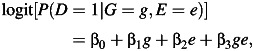 |
(1) |
where D is the disease outcome variable, G is the genetic factor, and E is the environmental factor. The joint test would then be a test of the joint null hypothesis that both the genetic main effect and the gene-environment interaction effect are zero (i.e., that β1 = β3 = 0). This null hypothesis might then be tested by using a likelihood ratio test. It has been shown that such a joint test has more power to detect genetic effects than does a marginal test of association between disease and the genetic variant, over a broad range of—though not all—scenarios (8).
What happens to this joint test under environmental confounding? Let us first suppose that the genetic variant affects the environmental factor itself and that there is an unmeasured confounding variable of the relationship between the environmental factor and the disease outcome, as in Figure 1A. Suppose that neither the genetic variant nor the environmental factor has any effect on the disease itself. In this case, the genetic variant and the disease outcome will be unassociated marginally. A test for marginal association between the genetic factor and the disease will have valid type I error. What happens to the joint test in this case? Unfortunately, under environmental confounding, the joint test at significance level α will in general reject the null with far greater frequency than the nominal significance level. We demonstrate this below through simulations but we can also see why this might be so analytically.
Figure 1.

Causal diagrams (A–D) illustrating when environmental confounding will bias joint tests and interaction tests but not marginal tests of genetic association. D, outcome; E, environmental factor; G, genetic variant; U, unmeasured environmental confounder.
In the setting of Figure 1A, G and D are unassociated marginally but both are also associated with E marginally. If 2 binary variables are unassociated marginally, and both are marginally associated with a third binary variable, then the 2 binary variables will be conditionally associated with each other within at least 1 stratum of the third variable; thus, in Figure 1A, G and D will be associated conditionally within at least 1 stratum of E. The phenomenon is sometimes described in the graphical modeling literature as one of “collider stratification” or “conditioning on a common effect” (17–20): Two variables, even if marginally uncorrelated, will in general be correlated conditional on the common effect. Suppose, for instance, that the mechanism for E in Figure 1A is that E occurs if at least 1 of U (unmeasured environmental confounder) or G is present. Although U and G may be uncorrelated in the population, conditioning on E = 1, for example, will induce correlation because if for a particular subject we had that E = 1 and U = 0, then we would know that G must be 1 for that subject since E occurs only if at least one of U and G is 1. Likewise, for a subject E = 1 and G = 0, we would know that U = 1. The variables U and G will thus be correlated conditional on E.
The implication of this for the logistic regression model 1 is that, under Figure 1A, without controlling for U, at least one of β1 or β3 will be nonzero. In other words, in large samples, the joint test will reject the null hypothesis β1 = β3 = 0 even though neither G nor E has any effect on D. This occurs because of the environmental confounder U for which control has not been made. Unfortunately, this problem gets worse as the sample size increases. Because the value of either β1 or β3 is nonzero (having not controlled for U), the joint test will reject the null β1 = β3 = 0 with a probability tending toward 1 as the sample size increases. We also illustrate this below through simulations. In Figure 1A, the marginal test for G would be valid, but the joint test will be biased. If we could control for the environmental confounder U in the analysis, our joint test would be valid for detecting genetic effects; without such control, we get an inconsistent test.
Joint tests under environmental confounding with gene-environment independence
Consider now Figure 1B in which the genetic and environmental factors are marginally independent in the population. In this case, under the null hypothesis that G has no effect on D, the joint test is protected against unmeasured environmental confounding under the null. The variable U may induce correlation between E and D, even if E itself has no effect on D. However, conditional on E, if G has no effect on E and no effect on D, then G will remain uncorrelated with D within all strata of E. Thus, under logistic regression model 1, if G has no effect on E and no effect on D, then both β1 and β3 will be zero. The joint test of a main genetic effect and a gene-environment interaction (e.g., the likelihood ratio test that β1 = β3 = 0) will maintain valid type I error under the null that there is no effect of the genetic variant on the disease, even in the presence of unmeasured environmental confounding, provided we have marginal gene-environment independence. Thus far, we have been considering joint tests for main genetic effects and gene-environment interaction, but similar principles in fact apply if the gene-environment interactions themselves are of intrinsic interest, rather than just being used to boost the power of tests to detect gene-disease associations.
Gene-environment interactions under environmental confounding
Suppose now that the genetic and environmental factors did in fact have effects on the disease outcome, as in Figure 1C, and that we were interested in assessing the extent to which the effect of the environmental factors varied according to the level of the genetic factor. That is, on the multiplicative scale of the logistic regression model in 1, we were interested in estimating the gene-environment interaction parameter β3. The interaction parameter β3 measures the ratio between 1) the odds ratio for disease when both the genetic and environmental factors are present and 2) the product of the odds ratios for disease when just the environmental or just the genetic factor is present. In general, if the environmental confounder U is not controlled for, this will bias estimates of the effect of E on D, and this will in turn also bias estimates of the gene-environment interaction parameter.
However, as before, some important exceptions occur in the presence of gene-environment independence. The results that follow assume a rare outcome as in most case-control studies. Suppose we have gene-environment independence in the population, as in Figure 1D, in the sense that G is independent of E and U marginally. Suppose further that the environmental confounder U does not interact with G on the multiplicative scale in its effects on D. It then follows that the interaction parameter estimate of β3 in logistic regression 1, ignoring the environmental confounder U, will be consistent for the true multiplicative interaction between G and E, controlling for U (21). The main effects for G and for E (β1 and β2) may still be biased, but the interaction parameter will be valid. This result holds even if U and E interact in their effects on D. The result, however, does depend on U and G not interacting in their effects on D. Because of gene-environment independence, this may be a reasonable assumption since U itself is assumed to be an environmental factor, but it certainly is not guaranteed to hold. The result does, however, again depend also on the assumption of gene-environment independence.
There is another interesting implication of this result. Under gene-environment independence, the estimate β3 in logistic regression 1 will be consistent (even ignoring U) if U and G do not interact on the multiplicative scale in their effects on D. Suppose then that we had an estimate of β3 that was nonzero; then, subject to sampling variability, it would follow that we must have gene-environment interaction either between G and E or between G and U (21). Essentially under gene-environment independence, the only way to have a nonzero interaction parameter is for some form of gene-environment interaction to be present, either with the environmental factor of interest or with some confounder of it. Similar results hold for measures of additive gene-environment interaction, further discussion of which is given elsewhere (21).
Similar principles also apply to case-only estimators of gene-environment interaction (22–25). These estimators assume that the genetic and environmental factors are independent. If, in addition, G is assumed to be independent of U, then first, if G does not interact with U on the multiplicative scale, the case-only estimator of the multiplicative interaction between G and E will be consistent even if we do not control for U (21); and second, if we do have a nonzero case-only gene-environment interaction parameter, then, even without assuming no interaction between G and U, we would be able to conclude some form of gene-environment interaction, either between G and E or between G and U. Again, these results depend on the assumption of gene-environment independence, but, with the case-only estimator, the performance of the estimator itself depends critically on the assumption of gene-environment independence even in the absence of environmental confounding (26).
Simultaneous testing for marginal genetic association and gene-environment interaction under environmental confounding
Alternatives to the joint test have been proposed to detect the involvement of a genetic factor in terms of its marginal association with disease and/or involvement in gene-environment interaction. In recent studies (9), proposals have been made to consider the 2 logistic regression models. The first uses a model for D-G association:
| (2) |
to test the marginal genetic effect, α1 = 0. The second uses model 1 above to test for the gene-environment interaction, β3 = 0. We denote the estimator of β3 as  to indicate fitting model 1 by using case-control data. Because the Wald χ2 test statistic for testing marginal genetic effect and the gene-environment interaction are independent (9), they can be combined to propose a χ22df test of the following form:
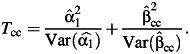 |
(3) |
Furthermore, modifications of this test were proposed by Dai et al. (9) by using alternative estimators for the gene-environment interaction parameter β3 that make use of the assumption of gene-environment independence. Several of these alternatives including the classic case-control, the case-only, and the empirical Bayes method were compared in a simulation study by Mukherjee et al. (27, 28), and we will consider these methods again here both in terms of the implications of environmental confounding and as alternatives for joint tests in the simulation study. The case-control method is robust but lacks power for testing G-E interaction. On the other hand, the case-only method provides substantial power gain over the case-control method under the gene-environment independence assumption but incurs severe type 1 error under violations of this assumption. The empirical Bayes method is a hybrid compromise that combines the case-control and case-only estimators with data-adaptive weights that optimally tradeoff between bias and efficiency under departures from the independence assumption. The empirical Bayes approach provides substantial power advantages compared with the case-control method and has far superior control of type I error compared with the case-only method under several scenarios of gene-environment association and moderate study sizes (27). The empirical Bayes estimator converges to the case-control estimator for large sample sizes.
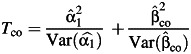
In constructing these various combined tests for marginal genetic association and gene-environment interaction (9), we found that the standard case-control estimator of gene-environment interaction,  in equation 3, can be replaced by these alternative estimators like the case-only estimator (denoted by
  ) or the empirical Bayes estimator (denoted by
  ) of the interaction parameter. The independence of the 2 test statistics still holds (9), and the marginal test and different gene-environment tests can be combined to give rise to 2 modifications of the 2-df tests:
 |
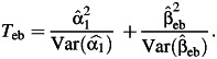 |
We refer to the 3 procedures mentioned above as the marginal genetic association + case-control, marginal genetic association + case-only, and marginal genetic association + empirical Bayes, respectively. Since environmental confounding affects the estimation of the gene-environment interaction parameter, we expect these combined tests also to behave similarly to the joint test. Moreover, the marginal genetic association + case-only procedure and, to a lesser extent, the marginal genetic association + empirical Bayes procedure will be affected by violation of the gene-environment independence assumption, as has been well characterized in the literature (26–28).
SIMULATION STUDY AND RESULTS
We carry out a simulation study to illustrate the type 1 error properties of the different tests under the global null hypotheses of H0: β1 = β2 = β3 = 0, in the presence of environmental confounding and under different scenarios of gene-environment association. We then consider estimation properties of the different approaches, namely, case-control, case-only, and empirical Bayes estimators of the gene-environment interaction parameter, β3, when there is nonnull interaction present. We report bias and empirical coverage properties of the estimated 95% confidence intervals with respect to the true parameter value (i.e., the proportion of times that the confidence intervals contains the true parameter) under varying scenarios of environmental confounding and gene-environment association.
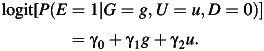
To numerically illustrate our results, we consider the setting of a case-control study with disease status D, binary G, E, and unmeasured environmental confounder U. We assume the disease to be rare. We first generate independent binary genetic factor G and unmeasured environmental confounder U with given prevalence. Given G and U, we generate the observed environmental factor E in the controls following a logistic model:
 |
(4) |
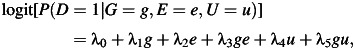
The parameters γ0, γ1, γ2 are chosen to maintain the desired values of P(E = 1), the G-E association as measured by the odds ratio of genetic factor, G, and environmental factor, E (ORGE), in controls, and the strength of the E and U association. Data are simulated in this manner so that the G-E association measure is among the controls; the assumption that G and E are independent among the controls is the exact assumption needed for the case-only estimator in logistic regression (22); with a rare disease, this assumption is approximately equivalent to G-E independence in the population. Given the cell probability configuration of (G,E,U|D = 0) and a disease risk model of the form
 |
(5) |
the distribution (G,E,U|D = 1) is generated as described (29). Note that in model 5, in order to generate environmental confounding of different forms, we include the terms involving D-U association and the possibility of G × U interaction by setting the values of the λ4 and λ5 parameters to nonzero value.
Type 1 error rates are estimated by empirical proportion of rejection of null hypotheses in 5,000 simulated data sets. Bias and empirical coverage probabilities are empirically estimated for the nonnull case based on 5,000 simulated data sets as well.
Inflation of type I errors under environmental confounding
Table 1 shows the type I error rates corresponding to the 4 joint tests (joint likelihood ratio test for β1 = β3 = 0 in model 1, denoted by G-GE, along with marginal genetic association + case-control, marginal genetic association + case-only, and marginal genetic association + empirical Bayes); the likelihood ratio test for β3 = 0 in model 1 (denoted by GE); and the marginal test of α1 = 0 in model 2 (denoted by G). In this setting, there is no G × U interaction or λ5 = 0 in model 5. We consider different degrees of environmental confounding (γ2 = λ4 = 0, log(2), log(5)) and different gene-environment association (ORGE = 1.0, 1.5, 2.0). Data were simulated under the global null hypothesis H0: λ1 = λ2 = λ3 = 0, that ensures a valid null for the marginal association tests in model 2. Under G-E independence, or ORGE = 1, type I errors for all tests maintain the nominal level (α = 0.05) even when the environmental confounder is ignored in the analysis. When G and E are associated with ORGE = 1.5 or 2.0 and when there is no unmeasured environmental confounding (γ2 = λ4 = 0), all tests maintain valid type I error rates except marginal genetic association + case-only and marginal genetic association + empirical Bayes. However, in the presence of G-E association, the joint test G-GE has inflated type I error when environmental confounding is present (γ2 = λ4 > 0). The test of no gene-environment interaction effect (GE) and the simultaneous test of marginal genetic effect and case-control interaction (marginal genetic association + case-control) also exhibit significant inflation of type I errors when the confounder effect is large. In this setting, marginal genetic association + case-control and marginal genetic association + empirical Bayes have less inflated type I error rates than G-GE or marginal genetic association + case-only. Moreover, the joint tests incorrectly reject the null more often as the sample size increases, confirming numerically that these tests reject the null with a probability that tends to 1 as the sample size increases. The marginal test of association remains valid (Table 1).
Table 1.
Type I Errors for 5 Association/Interaction Tests Across a Range of Environmental Confounder Effects and Sample Sizesa
| ORGE | γ2 = λ4b | No. of Cases and Controls | Test for Both G and G × E Effectsc |
GEd | Ge | |||
|---|---|---|---|---|---|---|---|---|
| G-GE | MA + CC | MA + CO | MA + EB | |||||
| 1.0 | 0 | 1,000 | 0.055 | 0.053 | 0.055 | 0.051 | 0.050 | 0.050 |
| 5,000 | 0.050 | 0.049 | 0.055 | 0.053 | 0.056 | 0.052 | ||
| 10,000 | 0.051 | 0.051 | 0.048 | 0.043 | 0.051 | 0.049 | ||
| log(2) | 1,000 | 0.054 | 0.054 | 0.052 | 0.042 | 0.067 | 0.048 | |
| 5,000 | 0.054 | 0.049 | 0.053 | 0.053 | 0.051 | 0.045 | ||
| 10,000 | 0.056 | 0.059 | 0.046 | 0.043 | 0.064 | 0.051 | ||
| log(5) | 1,000 | 0.047 | 0.048 | 0.055 | 0.047 | 0.031 | 0.048 | |
| 5,000 | 0.053 | 0.057 | 0.060 | 0.058 | 0.052 | 0.051 | ||
| 10,000 | 0.048 | 0.048 | 0.041 | 0.040 | 0.049 | 0.050 | ||
| 1.5 | 0 | 1,000 | 0.048 | 0.046 | 0.749 | 0.067 | 0.046 | 0.054 |
| 5,000 | 0.055 | 0.048 | 1.000 | 0.044 | 0.047 | 0.053 | ||
| 10,000 | 0.045 | 0.044 | 1.000 | 0.042 | 0.052 | 0.045 | ||
| log(2) | 1,000 | 0.063 | 0.058 | 0.749 | 0.082 | 0.055 | 0.052 | |
| 5,000 | 0.046 | 0.045 | 1.000 | 0.050 | 0.041 | 0.053 | ||
| 10,000 | 0.071 | 0.059 | 1.000 | 0.060 | 0.057 | 0.050 | ||
| log(5) | 1,000 | 0.067 | 0.049 | 0.807 | 0.073 | 0.048 | 0.048 | |
| 5,000 | 0.175 | 0.058 | 1.000 | 0.075 | 0.070 | 0.059 | ||
| 10,000 | 0.286 | 0.076 | 1.000 | 0.091 | 0.077 | 0.045 | ||
| 2.0 | 0 | 1,000 | 0.052 | 0.046 | 0.995 | 0.052 | 0.043 | 0.050 |
| 5,000 | 0.046 | 0.042 | 1.000 | 0.043 | 0.047 | 0.048 | ||
| 10,000 | 0.049 | 0.042 | 1.000 | 0.043 | 0.049 | 0.049 | ||
| log(2) | 1,000 | 0.047 | 0.044 | 0.997 | 0.050 | 0.056 | 0.048 | |
| 5,000 | 0.072 | 0.048 | 1.000 | 0.051 | 0.063 | 0.051 | ||
| 10,000 | 0.089 | 0.056 | 1.000 | 0.059 | 0.045 | 0.050 | ||
| log(5) | 1,000 | 0.117 | 0.051 | 0.999 | 0.066 | 0.057 | 0.045 | |
| 5,000 | 0.440 | 0.086 | 1.000 | 0.096 | 0.103 | 0.045 | ||
| 10,000 | 0.728 | 0.114 | 1.000 | 0.129 | 0.129 | 0.052 | ||
Abbreviation: ORGE, odds ratio of genetic factor, G, and environmental factor, E.
a We consider P(G = 1) = 0.3, P(E = 1) = 0.4, and P(U = 1) = 0.5 and generate data with λ1 = λ2 = λ3 = λ5 = 0 in disease risk model 5 for all settings. The nominal type 1 error level is set at α = 0.05. Results are based on 5,000 simulated data sets.
b γ2, the environmental confounder effect parameter in model 4; λ4, the environmental confounder effect parameter in disease risk model 5.
c G-GE, the joint likelihood ratio test for H0: β1 = β3 = 0 in model 1; marginal association test (MA) + case-control (CC), MA + case-only (CO), and MA + empirical Bayes (EB), the simultaneous 2-df tests for marginal genetic effect and gene-environment interaction, with the interaction test using the case-control, case-only, or empirical Bayes method.
d GE, the likelihood ratio test for H0: β3 = 0 in model 1.
e G, the likelihood ratio test for H0: α1 = 0 in model 2.
Bias in estimation of gene-environment interaction under environmental confounding but with no G × U interaction
Table 2 displays the bias in the parameter estimates for nonnull gene-environment interaction (β3) and the corresponding empirical coverage probability of the 95% Wald-type confidence interval using standard case-control  , case-only
  , or empirical Bayes
  estimator of the gene-environment interaction parameter under settings with uncontrolled environmental confounding with γ2 = λ4 = log(5) but no interaction between the environmental confounder and the gene. As expected, the interaction effect estimate is consistent, and the empirical coverage probability is maintained at the nominal level for all 3 estimators when the assumption of gene-environment independence holds (ORGE = 1), even in the presence of environmental confounding. Bias starts to increase and the empirical coverage probability starts to decrease for all 3 estimators when the independence assumption is not satisfied (ORGE > 1), though this occurs for case-only and empirical Bayes even in absence of environmental confounding (26–28). The standard case-control estimate is least affected, while the empirical Bayes estimator performs similarly in larger sample sizes.
Table 2.
Bias With Environmental Confounding but Without G × U Interactiona
| ORGE |  |
No. of Cases and Controls |
|
 |
 |
|||
|---|---|---|---|---|---|---|---|---|
| Bias | Coverage | Bias | Coverage | Bias | Coverage | |||
| 1.0 | log(1.2) | 1,000 | −0.001 | 0.946 | −0.004 | 0.958 | −0.004 | 0.965 |
| 5,000 | 0.000 | 0.963 | 0.001 | 0.958 | 0.000 | 0.967 | ||
| 10,000 | −0.003 | 0.948 | −0.003 | 0.945 | −0.003 | 0.967 | ||
| log(1.5) | 1,000 | 0.008 | 0.937 | 0.004 | 0.946 | 0.006 | 0.961 | |
| 5,000 | 0.004 | 0.957 | 0.004 | 0.947 | 0.004 | 0.966 | ||
| 10,000 | 0.000 | 0.958 | 0.000 | 0.961 | 0.000 | 0.968 | ||
| log(2.0) | 1,000 | 0.006 | 0.946 | −0.001 | 0.933 | 0.003 | 0.951 | |
| 5,000 | 0.000 | 0.959 | 0.001 | 0.940 | 0.001 | 0.959 | ||
| 10,000 | 0.001 | 0.938 | 0.000 | 0.943 | 0.000 | 0.956 | ||
| 1.5 | log(1.2) | 1,000 | 0.033 | 0.947 | 0.438 | 0.075 | 0.107 | 0.903 |
| 5,000 | 0.028 | 0.943 | 0.436 | 0.000 | 0.046 | 0.925 | ||
| 10,000 | 0.032 | 0.907 | 0.435 | 0.000 | 0.041 | 0.894 | ||
| log(1.5) | 1,000 | 0.036 | 0.938 | 0.442 | 0.084 | 0.110 | 0.899 | |
| 5,000 | 0.028 | 0.944 | 0.435 | 0.000 | 0.045 | 0.929 | ||
| 10,000 | 0.028 | 0.935 | 0.434 | 0.000 | 0.037 | 0.919 | ||
| log(2.0) | 1,000 | 0.029 | 0.952 | 0.432 | 0.116 | 0.105 | 0.909 | |
| 5,000 | 0.031 | 0.947 | 0.438 | 0.000 | 0.049 | 0.926 | ||
| 10,000 | 0.031 | 0.915 | 0.436 | 0.000 | 0.040 | 0.895 | ||
| 2.0 | log(1.2) | 1,000 | 0.053 | 0.932 | 0.747 | 0.000 | 0.105 | 0.907 |
| 5,000 | 0.052 | 0.910 | 0.746 | 0.000 | 0.063 | 0.893 | ||
| 10,000 | 0.055 | 0.851 | 0.745 | 0.000 | 0.060 | 0.834 | ||
| log(1.5) | 1,000 | 0.056 | 0.953 | 0.752 | 0.000 | 0.108 | 0.927 | |
| 5,000 | 0.049 | 0.930 | 0.741 | 0.000 | 0.060 | 0.904 | ||
| 10,000 | 0.050 | 0.862 | 0.743 | 0.000 | 0.056 | 0.844 | ||
| log(2.0) | 1,000 | 0.058 | 0.954 | 0.753 | 0.000 | 0.112 | 0.929 | |
| 5,000 | 0.051 | 0.901 | 0.742 | 0.000 | 0.062 | 0.887 | ||
| 10,000 | 0.049 | 0.878 | 0.741 | 0.000 | 0.054 | 0.862 | ||
Abbreviation: ORGE, odds ratio of genetic factor, G, and environmental factor, E.
a Bias and empirical coverage probability of the 95% confidence interval corresponding to the gene-environment interaction parameter, β3, using standard case-control  , case-only
  , and empirical Bayes
  estimator in the presence of environmental confounding with no interaction between the unmeasured confounder and gene. We generate data under P(G = 1) = 0.3, P(E = 1) = 0.4, and P(U = 1) = 0.5 and λ1 = log(1.2), λ2 = λ5 = 0, and λ4 = log(5) in disease risk model 5 for all settings. The effect of U on E or γ2 in model 3 is also set at log(5). Results are based on 5,000 simulated data sets.
b λ3, the gene-environment interaction parameter in disease risk model 5.
Bias in estimation of gene-environment interaction under environmental confounding and with G × U interaction
Table 3 shows the same results when there are environmental confounding and a G × U interaction, namely, λ5 = log(2) in model 5. In contrast to Table 2, the interaction effect estimate is biased, and the empirical coverage probability is reduced substantially for  ,
,  , and
, and  even under gene-environment independence (ORGE = 1). Among the 3 estimators, the undercoverage of the confidence interval for β3 using the case-only study design
  is the most serious, even under the independence of G and E. The standard case-control and empirical Bayes estimators perform similarly, especially at larger sample sizes.
Table 3.
Bias With Environmental Confounding and G × U Interactiona
| ORGE | |
No. of Cases and Controls |
 |
 |
 |
|||
|---|---|---|---|---|---|---|---|---|
| Bias | Coverage | Bias | Coverage | Bias | Coverage | |||
| 1.0 | log(1.2) | 1,000 | 0.111 | 0.915 | 0.112 | 0.856 | 0.112 | 0.894 |
| 5,000 | 0.112 | 0.724 | 0.113 | 0.503 | 0.112 | 0.636 | ||
| 10,000 | 0.111 | 0.552 | 0.110 | 0.233 | 0.110 | 0.376 | ||
| log(1.5) | 1,000 | 0.121 | 0.888 | 0.110 | 0.863 | 0.115 | 0.883 | |
| 5,000 | 0.117 | 0.732 | 0.114 | 0.502 | 0.115 | 0.604 | ||
| 10,000 | 0.113 | 0.541 | 0.111 | 0.249 | 0.112 | 0.368 | ||
| log(2.0) | 1,000 | 0.107 | 0.905 | 0.111 | 0.851 | 0.109 | 0.880 | |
| 5,000 | 0.112 | 0.765 | 0.111 | 0.557 | 0.112 | 0.647 | ||
| 10,000 | 0.112 | 0.563 | 0.110 | 0.295 | 0.111 | 0.415 | ||
| 1.5 | log(1.2) | 1,000 | 0.150 | 0.884 | 0.558 | 0.010 | 0.223 | 0.800 |
| 5,000 | 0.150 | 0.587 | 0.556 | 0.000 | 0.168 | 0.519 | ||
| 10,000 | 0.155 | 0.283 | 0.559 | 0.000 | 0.164 | 0.239 | ||
| log(1.5) | 1,000 | 0.149 | 0.869 | 0.559 | 0.013 | 0.224 | 0.797 | |
| 5,000 | 0.150 | 0.581 | 0.555 | 0.000 | 0.168 | 0.522 | ||
| 10,000 | 0.153 | 0.306 | 0.558 | 0.000 | 0.162 | 0.267 | ||
| log(2.0) | 1,000 | 0.156 | 0.877 | 0.569 | 0.026 | 0.233 | 0.788 | |
| 5,000 | 0.156 | 0.593 | 0.557 | 0.000 | 0.175 | 0.520 | ||
| 10,000 | 0.147 | 0.345 | 0.556 | 0.000 | 0.157 | 0.306 | ||
| 2.0 | log(1.2) | 1,000 | 0.188 | 0.840 | 0.873 | 0.000 | 0.240 | 0.776 |
| 5,000 | 0.179 | 0.464 | 0.875 | 0.000 | 0.190 | 0.419 | ||
| 10,000 | 0.181 | 0.169 | 0.874 | 0.000 | 0.186 | 0.145 | ||
| log(1.5) | 1,000 | 0.168 | 0.866 | 0.871 | 0.000 | 0.221 | 0.813 | |
| 5,000 | 0.179 | 0.471 | 0.874 | 0.000 | 0.190 | 0.430 | ||
| 10,000 | 0.183 | 0.166 | 0.875 | 0.000 | 0.188 | 0.148 | ||
| log(2.0) | 1,000 | 0.180 | 0.860 | 0.875 | 0.000 | 0.236 | 0.806 | |
| 5,000 | 0.176 | 0.505 | 0.873 | 0.000 | 0.188 | 0.459 | ||
| 10,000 | 0.177 | 0.227 | 0.872 | 0.000 | 0.183 | 0.203 | ||
Abbreviation: ORGE, odds ratio of genetic factor, G, and environmental factor, E.
a Bias of the parameter estimate for gene-environment effect, β3, and the corresponding empirical coverage probability of the 95% confidence interval using the case-control  , case-only
  , or empirical Bayes
  interaction estimator when environmental confounder and its multiplicative interaction with gene are not controlled. We consider P(G = 1) = 0.3, P(E = 1) = 0.4, and P(U = 1) = 0.5 and λ1 = log(1.2), λ2 = 0, λ4 = log(5), and λ5 = log(2) in disease risk model 5 for all settings. Thus, this simulation setting allows for the G × U interaction. The effect of U on E or γ2 in model 3 is also set at log(5). Results are based on 5,000 simulated data sets.
b λ3, the gene-environment interaction parameter in disease risk model 5.
DISCUSSION
In this paper, we have presented a number of different results concerning the implications of environmental confounding for gene-environment interaction studies. We have shown that, if such confounding is left uncontrolled, joint tests for a genetic main effect are biased, but this problem dissolves under gene-environment independence, and the joint tests are again valid, even if the environmental confounding is left uncontrolled. Even under gene-environment independence, uncontrolled environmental confounding can bias estimates of gene-environment interaction parameters, unless the unmeasured environmental confounder does not itself interact with the genetic factor.
The results of this paper have several implications for the conduct of gene-environment interaction studies. Perhaps the most important is that environmental confounding should be taken seriously in studies of gene-environment interaction. Careful control is often made for genetic confounding by population stratification using principal components analysis or other methods (10–16). However, environmental confounding is frequently ignored in gene-environment interaction studies. Because of the severe nature of the biases that can arise from such environmental confounding, more careful thought should be given to what factors may be common causes of the environmental factor of interest and the disease under study. Efforts should be made at the data collection stage to measure such variables, and they should then be controlled for in the analysis in order to avoid the biases described in this paper.
Another important implication of the results here is that the extent of the bias that arises when environmental confounding is present and not controlled for depends critically on whether or not the genetic and environmental factors are marginally independent. Gene-environment independence does not completely alleviate bias due to environmental confounding in estimates of gene-environment interaction parameters, but it does mitigate considerably the settings in which such biases can arise. As seen above, with joint tests, violation of gene-environment independence can severely bias these tests. Unless a researcher is very sure that the gene-environment independence assumption holds, joint tests (leveraging an environmental factor for discovering new loci) should perhaps be avoided as they can be severely biased in the presence of environmental confounding. When they are used, the simultaneous tests (9) that combine a marginal test and a test using either a case-control estimator (marginal genetic association + case-control) or an empirical Bayes estimator (marginal genetic association + empirical Bayes) of the interaction parameter seemed least susceptible to the biases documented. The marginal genetic association + case-only approach suffers the most from violation of gene-environment independence and should be avoided if the researcher is uncertain of this assumption.
Gene-environment independence is commonly assumed in the literature and, in many cases, it is a reasonable assumption. However, when the tests are used for the purposes of detection, there may be insufficient knowledge to evaluate the assumption. Moreover, there are documented settings in which the genetic variants are related to both the environmental factor under study and also the disease outcome as, for example, was recently shown to be the case with the effect of variants on 15q25 on smoking and lung cancer (30–33). At this point, such settings are probably more the exception than the rule, and researchers are at least partially protected from environmental confounding by gene-environment independence. However, as personal knowledge of one's own genetic risk factors increases, if such knowledge leads to changes in behavior and environmental exposures, this gene-environment independence may no longer be preserved (34). The biases described in this paper will then also be more prominent.
Furthermore, even under gene-environment independence, environmental confounding can still give rise to bias in gene-environment interaction parameter estimates. Effort should be made to control for environmental confounding. When this is not possible, sensitivity analysis techniques for gene-environment interaction have been developed (21) to help assess the extent to which an unmeasured environmental confounder would have to be related to both the environmental factor of interest and the disease outcome to substantially change qualitative and quantitative inferences. We would recommend the use of these methods when it is not possible to control for environmental confounding. In the genome-wide association study and the post–genome-wide association study age, extraordinary technological development and advances in measurement have increased our capacity to evaluate and control for genetic factors and confounding that might be associated with them. Amidst this extraordinary progress, it is important not to lose sight of the other side to the story—the environment. Efforts should likewise be directed at the measurement of environmental factors and potential confounders, as well as at the analytical control for these confounders, when necessary, to eliminate bias and to help ensure accurate inferences.
ACKNOWLEDGMENTS
Author affiliations: Departments of Epidemiology and Biostatistics, Harvard School of Public Health, Boston, Massachusetts (Tyler J. VanderWeele); and Department of Biostatistics, University of Michigan School of Public Health, Ann Arbor, Michigan (Yi-An Ko, Bhramar Mukherjee).
The research was supported by grant ES017876 from the National Institutes of Health.
Conflict of interest: none declared.
REFERENCES
- 1.Hunter DJ. Gene-environment interactions in human diseases. Nat Rev Genet. 2005;6(4):287–298. doi: 10.1038/nrg1578. [DOI] [PubMed] [Google Scholar]
- 2.Chatterjee N, Mukherjee B, editors. Statistical Approaches to Studies of Gene-Gene and Gene-Environment Interaction. New York, NY: Informa HealthCare; 2008. [Google Scholar]
- 3.Murcray CE, Lewinger JP, Gauderman WJ. Gene-environment interaction in genome-wide association studies. Am J Epidemiol. 2009;169(2):219–226. doi: 10.1093/aje/kwn353. [DOI] [PMC free article] [PubMed] [Google Scholar]
- 4.Kraft P, Hunter DJ. The Challenge of Assessing Complex Gene-Gene and Gene-Environment Interactions. 2nd ed. New York, NY: Oxford University Press; 2009. [Google Scholar]
- 5.Thomas D. Gene-environment-wide association studies: emerging approaches. Nat Rev Genet. 2010;11(4):259–272. doi: 10.1038/nrg2764. [DOI] [PMC free article] [PubMed] [Google Scholar]
- 6.Garcia-Closas M, Jacobs K, Kraft P, et al. Analysis of epidemiologic studies of genetic effects and gene-environment interactions. IARC Sci Publ. 2011;(163):281–301. [PubMed] [Google Scholar]
- 7.Chatterjee N, Kalaylioglu Z, Moslehi R, et al. Powerful multilocus tests of genetic association in the presence of gene-gene and gene-environment interactions. Am J Hum Genet. 2006;79(6):1002–1016. doi: 10.1086/509704. [DOI] [PMC free article] [PubMed] [Google Scholar]
- 8.Kraft P, Yen YC, Stram DO, et al. Exploiting gene-environment interaction to detect genetic associations. Hum Hered. 2007;63(2):111–119. doi: 10.1159/000099183. [DOI] [PubMed] [Google Scholar]
- 9.Dai J, Logsdon B, Huang Y, et al. Simultaneous testing for marginal genetic association and gene-environment interaction in genome-wide association studies. Am J Epidemiol. 2012;176(2):164–173. doi: 10.1093/aje/kwr521. [DOI] [PMC free article] [PubMed] [Google Scholar]
- 10.Pritchard JK, Rosenberg NA. Use of unlinked genetic markers to detect population stratification in association studies. Am J Hum Genet. 1999;65(1):220–228. doi: 10.1086/302449. [DOI] [PMC free article] [PubMed] [Google Scholar]
- 11.Pritchard JK, Stephens M, Rosenberg NA, et al. Association mapping in structured populations. Am J Hum Genet. 2000;67(1):170–181. doi: 10.1086/302959. [DOI] [PMC free article] [PubMed] [Google Scholar]
- 12.Satten GA, Flanders WD, Yang QH. Accounting for unmeasured population substructure in case-control studies of genetic association using a novel latent-class model. Am J Hum Genet. 2001;68(2):466–477. doi: 10.1086/318195. [DOI] [PMC free article] [PubMed] [Google Scholar]
- 13.Hoggart CJ, Parra EJ, Shriver MD, et al. Control of confounding of genetic associations in stratified populations. Am J Hum Genet. 2003;72(6):1492–1504. doi: 10.1086/375613. [DOI] [PMC free article] [PubMed] [Google Scholar]
- 14.Price AL, Patterson NJ, Plenge RM, et al. Principal components analysis corrects for stratification in genome-wide association studies. Nat Genet. 2006;38(8):904–909. doi: 10.1038/ng1847. [DOI] [PubMed] [Google Scholar]
- 15.Bhattacharjee S, Wang Z, Ciampa J, et al. Using principal components of genetic variation for robust and powerful detection of gene-gene interactions in case-control and case-only studies. Am J Hum Genet. 2010;86(3):331–342. doi: 10.1016/j.ajhg.2010.01.026. [DOI] [PMC free article] [PubMed] [Google Scholar]
- 16.Price AL, Zaitlen NA, Reich D, et al. New approaches to population stratification in genome-wide association studies. Nat Rev Genet. 2010;11(7):459–463. doi: 10.1038/nrg2813. [DOI] [PMC free article] [PubMed] [Google Scholar]
- 17.Pearl J. Causality: Models, Reasoning, and Inference. 2nd ed. New York, NY: Cambridge University Press; 2009. [Google Scholar]
- 18.Cole SR, Platt RW, Schisterman EF, et al. Illustrating bias due to conditioning on a collider. Int J Epidemiol. 2010;39(2):417–420. doi: 10.1093/ije/dyp334. [DOI] [PMC free article] [PubMed] [Google Scholar]
- 19.VanderWeele TJ, Robins JM. Directed acyclic graphs, sufficient causes, and the properties of conditioning on a common effect. Am J Epidemiol. 2007;166(9):1096–1104. doi: 10.1093/aje/kwm179. [DOI] [PubMed] [Google Scholar]
- 20.Hernan MA, Hernandez-Diaz S, Robins JM. A structural approach to selection bias. Epidemiology. 2004;15(5):615–625. doi: 10.1097/01.ede.0000135174.63482.43. [DOI] [PubMed] [Google Scholar]
- 21.VanderWeele TJ, Mukherjee B, Chen J. Sensitivity analysis for interactions under unmeasured confounding. Stat Med. 2012;31(22):2552–2564. doi: 10.1002/sim.4354. [DOI] [PMC free article] [PubMed] [Google Scholar]
- 22.Piegorsch WW, Weinberg CR, Taylor JA. Non-hierarchical logistic-models and case-only designs for assessing susceptibility in population-based case-control studies. Stat Med. 1994;13(2):153–162. doi: 10.1002/sim.4780130206. [DOI] [PubMed] [Google Scholar]
- 23.Khoury MJ, Flanders WD. Nontraditional epidemiologic approaches in the analysis of gene-environment interaction: case-control studies with no controls! Am J Epidemiol. 1996;144(3):207–213. doi: 10.1093/oxfordjournals.aje.a008915. [DOI] [PubMed] [Google Scholar]
- 24.Schmidt S, Schaid DJ. Potential misinterpretation of the case-only study to assess gene-environment interaction. Am J Epidemiol. 1999;150(8):878–885. doi: 10.1093/oxfordjournals.aje.a010093. [DOI] [PubMed] [Google Scholar]
- 25.Yang Q, Khoury MJ, Sun F, et al. Case-only design to measure gene-gene interaction. Epidemiology. 1999;10(2):167–170. [PubMed] [Google Scholar]
- 26.Albert PS, Ratnasinghe D, Tangrea J, et al. Limitations of the case-only design for identifying gene-environment interactions. Am J Epidemiol. 2001;154(8):687–693. doi: 10.1093/aje/154.8.687. [DOI] [PubMed] [Google Scholar]
- 27.Mukherjee B, Ahn J, Gruber SB, et al. Tests for gene-environment interaction from case-control data: a novel study of type I error, power and designs. Genet Epidemiol. 2008;32(7):615–626. doi: 10.1002/gepi.20337. [DOI] [PubMed] [Google Scholar]
- 28.Mukherjee B, Ahn J, Gruber SB, et al. Testing gene-environment interaction in large-scale case-control association studies: possible choices and comparisons. Am J Epidemiol. 2012;175(3):177–190. doi: 10.1093/aje/kwr367. [DOI] [PMC free article] [PubMed] [Google Scholar]
- 29.Satten GA, Kupper LL. Inferences about exposure-disease associations using probability-of-exposure information. JASA. 1993;88(421):200–208. [Google Scholar]
- 30.Amos CI, Wu X, Broderick P, et al. Genome-wide association scan of tag SNPs identifies a susceptibility locus for lung cancer at 15q25.1. Nat Genet. 2008;40(5):616–622. doi: 10.1038/ng.109. [DOI] [PMC free article] [PubMed] [Google Scholar]
- 31.Hung RJ, McKay JD, Gaborieau V, et al. A susceptibility locus for lung cancer maps to nicotinic acetylcholine receptor subunit genes on 15q25. Nature. 2008;452(7187):633–637. doi: 10.1038/nature06885. [DOI] [PubMed] [Google Scholar]
- 32.Thorgeirsson TE, Geller F, Sulem P, et al. A variant associated with nicotine dependence, lung cancer and peripheral arterial disease. Nature. 2008;452(7187):638–642. doi: 10.1038/nature06846. [DOI] [PMC free article] [PubMed] [Google Scholar]
- 33.VanderWeele TJ, Asomaning K, Tchetgen Tchetgen EJ, et al. Genetic variants on 15q25.1, smoking, and lung cancer: an assessment of mediation and interaction. Am J Epidemiol. 2012;175(10):1013–1020. doi: 10.1093/aje/kwr467. [DOI] [PMC free article] [PubMed] [Google Scholar]
- 34.VanderWeele TJ. Genetic self knowledge and the future of epidemiologic confounding. Am J Hum Genet. 2010;87(2):168–172. doi: 10.1016/j.ajhg.2010.07.006. [DOI] [PMC free article] [PubMed] [Google Scholar]