A Mathematical Model on Water Redistribution Mechanism of the Seismonastic Movement of Mimosa Pudica

Abstract

A theoretical model based on the water redistribution mechanism is proposed to predict the volumetric strain of motor cells in Mimosa pudica during the seismonastic movement. The model describes the water and ion movements following the opening of ion channels triggered by stimulation. The cellular strain is related to the angular velocity of the plant movement, and both their predictions are in good agreement with experimental data, thus validating the water redistribution mechanism. The results reveal that an increase in ion diffusivity across the cell membrane of <15-fold is sufficient to produce the observed seismonastic movement.

Introduction

The quick reaction of Mimosa pudica to mechanical stimuli is referred to as seismonastic movement. Upon various stimuli, such as touching, heating, shaking, and electrical voltage, the plant can move rapidly via motor organs (1). These motor organs, termed pulvini, consist of the swollen joints found at three levels—a primary pulvinus at the joint between a petiole and the stem, the secondary pulvinus that joins a pinna with a petiole, and the tertiary pulvinus that joins a pinnule and a pinna (2). When the plant is stimulated, the straight pulvini would bend up or down, leading to three types of movement—the bending of the petioles, pinnae, and pinnules. In particular, the bending of its petioles and pinnules can reach 90° within a few seconds.

Compared to skeletal muscle which has a complicated structure and requires nerve and circulation systems to function, the motor organs responsible for rapid movement of M. pudica appear to be significantly simpler and standalone. This has aroused the attention of biological science researchers (3–5) as well as biophysicists and engineers because the movements can be inspiring in the design of actuators (6–8).

To mimic the plant, the possible mechanisms behind the seismonastic movement have to be investigated. One popular mechanism that explains this movement is related to the water redistribution mechanism in the motor organs: after the plant is stimulated, water in the pulvinar cells on one side (named extensor) will flux out, causing a loss in turgor that results in the bending of the pulvinus (2).

The mechanism is worthy of investigation not only because its fast movement and rapid response resemble artificial muscles such as conducting polymers (9,10), but also from a number of other reasons:

• 1.The movement is fast and yet observable by the eye, and greatly reduces the difficulty in measuring the speed of the movement.
• 2.The size of the motor organs is large enough for measurements and experiments using simple apparatus.
• 3.The geometry of the motor organs is simple and the movement is approximately in a single direction, thus reducing the complexity of mathematical modeling.

In this article, the cellular response in the largest motor organ—the primary pulvinus—is investigated through experiments and mathematical modeling. The experimental results and the model prediction will be compared to validate the mechanism.

Materials and Methods

Plants

Potted M. pudica L. used in these experiments were purchased from the market. Plants used for paraffin sections were incubated in a plant growth chamber under 23°C/21°C (day/night) cycles, and were watered daily. The plants for measurement of bending movement were grown indoors. All experiments were performed on ∼2-month-old healthy adult specimens.

Measurements on velocity of the seismonastic movement in M. pudica

In the seismonastic movements of M. pudica, the primary pulvinus deforms by downward bending (Fig. 1). The angles swept by the petiole were measured. The highest angle measured was 90 ± 2°, which is comparable to the measurement of 100° by Volkov et al. (11). Also, the angular velocity of the movement was estimated from the data obtained from the first measurement on three different days (M1–M3), and was plotted against time in Fig. 2. Although the peak values vary, it is clear that all curves show a similar trend.

Figure 1.

The deformation of the primary pulvinus and the bending of the petiole. (a) Original position. (b) Final position.

Figure 2.

The angular velocity versus time obtained from the experiment (M1–M3) with the prediction from the mathematical model. M1–M3 are the measurements from three different days and the prediction includes the upper and lower bound for the measurements. The values of constants and variables are L_w = 2.5 × 10⁻¹¹ ms⁻¹ Pa⁻¹; $c_{K_i}=250$ mM; $c_{C{l}_i}=100$ mM; θ₀ = 45°; d₀ = 4 mm; ϕ_i = 11 and 13 m s⁻¹; E = 3.5; and 7.0 MPa for upper and lower bound, respectively. The remaining constants are given in the last column of Tables 1 and 2.

To measure the angles swept by the petiole of M. pudica, the plant was stimulated and the movements were video-recorded. The movement was triggered by direct touching on the pulvinus by a needle and the angle swept by the petiole was measured by a protractor placed behind the plant.

From the video recording, the angular velocity of the bending was calculated by recording the time for the petiole to sweep through every 10°. The measurement was done on Windows Live Movie Maker (Microsoft, Redmond, WA), which has an accuracy of 0.01 s,. Taking into account the frame per second of the video (29 fps), the combined measurement error on time was 0.02 s. Considering further the measurement error on angles from the protractor, the total error is estimated to be 10–25%, the smaller error for the lower velocity, except for the every first measurement as the angle between the initial position and the first major marking being <10°.

Measurements on the volumetric strain of the cells in the primary pulvinus

In addition to the angular velocity of the petiole, the volumetric strains of the motor cells before and after deformation were measured using paraffin longitudinal sections of the pulvinus. Figs. 3 and 4 show representative slides of straight and curved sections, respectively. Evidently, the size of cells at the lower side of the curved section in Fig. 4 is the smallest in comparison to the upper side and at both sides of the straight pulvinus in Fig. 3, consistent with previous results (2,12,22). The measured percentage change on the areas between the straight (initial) and the curved (final) pulvinus reveals that the upper side (flexor) had increased by 7–17% and the lower side (extensor) had decreased by 20–38%. The large range in measurements for the extensor arose from errors in locating the cell walls.

Figure 3.

The microscopic pictures of a straight primary pulvinus. (a) Whole longitudinal section (bar, 200 μm). (b) Magnified upper part. (c) Magnified lower part of the pulvinus (bar, 50 μm).

Figure 4.

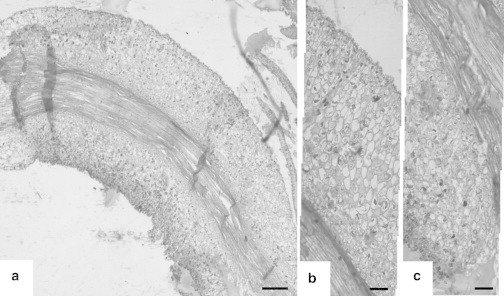
The microscopic pictures of a curved primary pulvinus. (a) Whole longitudinal section (bar, 200 μm). (b) Magnified upper part. (c) Magnified lower part of the pulvinus (bar, 50 μm).

To examine the motor cell size before bending movement, the plant was treated with ethyl ether vapor for 30 min (23). Paraffin sectioning was carried out according to the previous procedure described in Hong et al. (24) with some modifications. Pulvini of 0.4-cm lengths were cut and fixed with 4% paraformaldehyde in 0.1 M phosphate buffer (pH 7.2) for 16 h. The samples were then dehydrated by a series of increasing concentrations of ethanol solutions (30, 50, 70, and 85% for 2 h, followed by 95 and 100% for 2 h twice), ethanol-xylene mixture with the ratio of 2:1, 1:1, and 1:2 for 1 h each and pure xylene, twice, for 1 h each. The dehydrated samples were then infiltrated with paraffin twice, each for 1.5 h in a vacuum chamber at 62°C. The samples were then placed into embedding molds to which melted paraffin was poured. The paraffin blocks formed after cooling were then sectioned to a thickness of 7–10 μm using a microtome. The samples were laid on microscopic glass slides for dewaxing followed by staining.

Overview of the mathematical model

The objective of the mathematical model is to relate the deformation of the primary pulvinus to the opening of the ion channels in the cell membrane, to capture the essential features of the motor cell that include the zero net flux of water and ions at initial stationary state, the trigger of the ions and water fluxes, and the change in the volumetric strain of the cell.

The deformation of the primary pulvinus, as shown in Fig. 1, a and b, can be regarded as single degree-of-freedom involving the pure bending of the longitudinal section of the pulvinus. As a result, the movement of the primary pulvinus is approximated here as a transformation from a rectangular shape into a fan shape as shown in Fig. 5, which is directly related to the angle swept by the petiole in Fig. 1, a and b. Fig. 6 shows the cross section of an extensor cell which is assumed to be spherical. The cell contains the cell wall, the membrane, and the intracellular space (which is assumed to be homogeneous for simplicity). R and t are the radius of the cell and the cell wall thickness, respectively. P_i/o and Π_i/o are the water pressure and osmotic pressure in the intracellular or extracellular space of the cell, and both of the spaces contain K⁺, Cl⁻, water, and fixed charges. In a real cell, fixed charges reside on the solid network in the cytoplasm and cell wall, wheras in the model, the fixed charges are assumed to distribute evenly at both sides of the cell membrane. The fluxes of the two ions, K⁺ and Cl⁻, and that of water, are modeled, and the results of interest are the final volumetric strain of the cell and angular velocity of the petiole, because they can be compared with the experimental results.

Figure 5.

The approximated deformation of the longitudinal section of the primary pulvinus. The section deformed from rectangular into a fan-shaped plane with the neutral axis remaining in the middle.

Figure 6.

A single spherical extensor cell in the model. The cell contains the cell wall, membrane, and intracellular space. R and t are the radius of the cell and the cell wall thickness. P_i/o and Π_i/o are the water pressure and osmotic pressure in the intracellular or extracellular space, and both of the spaces contain K⁺, Cl⁻, water, and fixed charges.

Before the plant is stimulated, the membrane potential is known to be ∼−140 mV (−144 mV measured by Abe and Oda (25); −139 ± 12 mV by Fleurat-Lessard et al. (26)), which is more hyperpolarized (more negative) than that in the cortical parenchyma of the petiole (−52 mV by Sibaoka (27)) and in the stem (−61 ± 13 mV by Fleurat-Lessard et al. (26)). As for the ion concentration, Samejima and Sibaoka (18) and Kumon and Tsurumi (17) reported the extracellular concentration of K⁺ to increase from 27 to 200 mM, and that of Cl⁻ to increase from 10 to 80 mM, after the pulvinus has deformed. These results suggest that before the plant is stimulated, the intracellular concentrations of K⁺ and Cl⁻ are higher than the extracellular by possibly an order of magnitude of 100 mM.

The high intracellular concentrations of the ions in the extensor cells before the plant is triggered are maintained by trans-membrane active transport of ions, which balances the opposite passive transport through ion channels (see Eq. A8). The high intracellular ion concentrations lead to a high osmotic pressure inside the cell, and this is used to support the weight of the petiole. Thus, before the plant is stimulated, the transports are in a state of dynamic balance with no net flow of ions or water into the cell. Upon stimulation, as mentioned before, the ion channels in the cell membrane may be opened up, and the cell may also be depolarized. This would allow an instantaneous diffusional flux of ions outward of the cell under the high concentration and electric potential gradients across the cell membrane, thus causing the intracellular osmotic pressure to drop, and hence the weight of the petiole causes the pulvinus to bend downward. Such a movement is rapid (see Fig. 2) because this is the consequence of passive ion channels and transports. After the primary pulvinus has bent down fully, it will take a much longer time (∼1/2 h) to recover to its original erected position. The reason, in this picture, is that after the fast bending down, the ion concentrations and electric potential intra- and extracellular are more balanced and so the passive transports cease, and now the active trans-membrane transport mechanisms operate to pump ions back into the extensor cells, to erect the pulvinus again. The active transports are much slower and this explains the slow recovery.

In the following, the opening up of the ion channels upon stimulation is modeled by a step increase in the trans-membrane diffusive coefficient D_i of the ions, and the cell depolarization by a step drop in the trans-membrane electrical potential difference Δψ (Eq. A8). The direction of the active transport can be deduced from the difference between the membrane potential and the Nernst potential at the stationary state, and the magnitude of the active flux should be the negative of that of the passive flux.

Key assumptions of the model

• Assumption 1: The extensor cell is assumed to be spherical and contains a homogeneous and isotropic elastic cell wall, membrane, and intracellular space.

• Assumption 2: The fixed charges are assumed to distribute evenly at both sides of the cell membrane.

• Assumption 3: The cell considered is embedded in a large extracellular medium containing different ion concentrations compared to that in the intracellular space.

• Assumption 4: The volume contained by the cell membrane is equal to the water volume only, whereas the volume of ions and all the intracellular structures is neglected.

• Assumption 5: Intracellular and extracellular diffusion takes place over a timescale much faster than the ion flux across the cell membrane, so that the intracellular and extracellular ion concentrations become uniform quickly and only the ion flux across the cell membrane is modeled. The extracellular medium includes the cell wall.

• Assumption 6: As water flows across the membrane mainly through the water channels (aquaporins) while the ions pass through the membrane via ion channels, the coupling between the ion and water movements is neglected.

• Assumption 7: It is assumed that the cell is always spherical throughout the simulation.

Details of the model

The governing equations for the volume flow J_v [m s⁻¹] and the ion flows J_i[mol m⁻² s⁻¹] are given as Eqs. 39 and 41 from Kedem and Katchalsky (28), which were derived from an irreversible thermodynamic approach for a system with a solvent, a permeable solute, and impermeable solutes contained in two compartments separated by a semipermeable membrane:

$$J_v=L_p\left[\Delta p-\Delta {\Pi }_i-\sigma \left(\overline{R}T\Delta c_s+\phi \Delta {\Pi }_i\right)\right],$$ (1)

$$J_i=J_v\left(1-\sigma \right)c_s+\omega \left(\overline{R}T\Delta c_s+\phi \Delta {\Pi }_i\right).$$ (2)

Here J_v is the volume flow composed of the solvent and solute flow, L_p is the phenomenological coefficient relating the flow and the driving force, σ is the reflection coefficient, ω is the mobility of the solute, c_s is the mean of the concentrations of the solute in the two compartments, φ is the volume fraction of the solute, $\overline{R}T$ is the gas constant times the temperature in absolute scale, and Δp, ΔΠ_i, and Δc_s are the hydrostatic pressure difference, osmotic pressure difference induced by the impermeable solutes, and the concentration difference of the permeable solute across the membrane, respectively.

In our model, J_v would not be considered in Eq. 2 due to Assumption 6; and as the model only considers permeable solutes, ΔΠ_i in Eqs. 1 and 2 vanish. Moreover, as the solutes considered are charged, the driving force of their flow should also include the electrical potential difference across the membrane. As a result, the governing equation for the volume flow in the model is given by

$$J_w=L_w\left(\Delta \Pi -\Delta P\right),$$ (3)

where ΔΠ is the osmotic pressure difference and ΔP is the water pressure difference across the cell membrane. Because the dynamic pressure profile, derived from the inviscid Navier-Stokes equation in Appendix, is independent of r, ΔP equals the hydrostatic pressure difference. The time derivative of the cell radius $\dot{R}$ is equal to −J_w (see Appendix), therefore

$$\dot{R}=-L_w\left[\Delta \Pi -\Delta P\right].$$ (4)

With the governing equation for the ion flow across the cell membrane J_i[mol m⁻² s⁻¹], and the initial conditions of ion concentrations, the problem is closed. However, to validate the model by the experimental results, the volumetric strain rate of the cell predicted by the model needs to be related to the angular velocity of the petiole. As mentioned above, the deformation of the pulvinus is considered as a transformation of a rectangular longitudinal section into a fan-shape section with the neutral axis remaining in the middle (Fig. 2). Moreover, it is assumed that no deformation occurred in the transverse section. As a result, the angle swept by the petiole θ can be related to the change in length δd(y, t) of the section along the y direction by δd(y, t) = yθ(t). Also, the change in radius of the cell during the bending is proportional to δd. Therefore, the volumetric strain rate ${\dot{\Phi }}_V$ can be expressed in terms of the angular velocity $\dot{\theta }$ of the petiole as

$${\dot{\Phi }}_V=K\left(y,\theta \right)\dot{\theta }\left(t\right),$$ (5)

where K(y,θ) = 3(y/d₀)³θ² + 6(y/d₀)²θ + 3y/d₀. As stated above, y is taken as 1 mm, and the initial angle θ₀ = 45° and d₀ = 4 mm can be used, which are the measured values of the plant used for the experiments.

The governing equations were solved numerically (details given in Appendix). As mentioned beforehand, the cell is at a stationary state initially, at which there is no net flux of ions and water across the cell membrane. The fluxes of ions and water are triggered by replacing the ions’ diffusive coefficient D_i by a larger value D^′_i, which represents the opening of ion channels, and a decrease in the electrical potential difference across the cell membrane (Δψ), which represents the depolarization of the cell. These two processes are the possible causes of the water redistribution mechanism.

Moving mechanism

As reviewed by Volkov et al. (11), there are several hypothetical mechanisms suggested for the seismonastic movement of M. pudica, and a number of processes were found to be closely related to its movement. For the present study, the focus was on the water redistribution mechanism, which has been supported by the NMR results by Tamiya et al. (12), who showed that water would flux from the pulvinar cells on the lower side (extensor) to the upper (flexor) of the primary pulvinus.

Two possible causes of the water redistribution have been proposed. In one theory, certain chemical compounds (turgorins) open the ion channels on motor cells and hence alter the turgor pressure of the cells (13–15). In another hypothesis, K⁺ and Cl⁻ voltage-gated ion channels are activated by an action potential and the turgor of the cells would be altered due to the change in the concentration of ions across the cell membranes of the motor cells (3,11). More supportive evidence has been provided for the latter hypothesis, including the experimental results on the amount of ions efflux (16–18), the sensitivity of the plant to the chemicals that decrease K⁺ current (19) and the excitability of the extensor cells (20).

In the mathematical model proposed in this article, the opening of ion channels is represented by an initial increase in the ion permeability across the cell membrane. Such a condition can be the consequence of either of the above hypotheses for water redistribution and so the predicted results would not be able to test the correctness of both hypotheses. However, the model will be useful to prove the correctness of the water redistribution mechanism. Also, it can determine the contribution from an increase in the membrane potential, which is the electrical potential difference across the membrane of a biological cell, caused by the action potential. It should be noted that a previous hydroelastic curvature model also offers a quantitative picture for the movements of M. pudica (3) and Venus flytrap (Dionaea muscipula Ellis) (21) by focusing on the shape change of two layers of cells behaving like a bilayer couple. However, the present model aims at relating the bending of M. pudica with the flux of ions and water of single cells, thus serving as a test for the water redistribution mechanism.

Two unresolved issues concerning the water redistribution will be answered by the model, namely, whether the water flux is quick enough to cause the bending of the pulvinus, and whether the ion efflux is large enough to create a pressure gradient to cause the water flux. These questions not only provide the key in understanding the mechanism of seismonastic movements, but are also potentially important in shedding light on the design of novel types of artificial materials for intelligent robotics.

Results and Discussion

The objective of the mathematical model is to compute the volumetric strain of an extensor cell and the angular velocity of petiole for direct comparison with the experimental results. The volumetric strain and its rate were calculated from the radius R governed by Eq. 4, and the angular velocity $\dot{\theta }$ was obtained from the volumetric strain rate by Eq. 5. As the factor K in Eq. 5 is monotonically increasing with θ, the area under the curve of $\dot{\theta }\left(t\right)$ can serve as a quick indication of the final volumetric strain of the cell.

Effects of material constants

The prediction of the model depends on several material constants, including the elastic modulus E and the Poisson’s ratio v of the cell wall, the coefficient of hydraulic permeability for the water flow L_w, and the initial and triggered diffusive coefficients for ion flows D_i and D^′_i. As large ranges for these constants could be found in the literature, a discussion on their effects will be necessary for a better understanding on the results. The ranges of the constants used are given in Table 1, and the last column for each constant is the value used for the trials of other constants.

Table 1.

Range of constants used in the model

Symbol of the constant [unit]	Range of the magnitude	Value for the trials of other constants
E[Pa]a	1 × 104–1 × 108f	1 × 106
vb	0–0.5	0
Lw [m s−1 Pa−1]c	1 × 10−14–1 × 10−11g	1 × 10−11
LK, LCl [m s−1]d	1 × 10−7–1 × 10−9h	1 × 10−7
ϕK, ϕCle	1–100	10

The first and second columns are the symbol and the range of magnitude of the constant. The last column for each constant is the value used for the trials of other constants.

^aElastic modulus of cell wall.

^bPoisson’s ratio of cell wall.

^cPermeability for water.

^dInitial permeability for K⁺ and Cl⁻.

^eRatio of triggered to initial permeability of K⁺ and Cl⁻.

^fRanges obtained from Gibson (30).

^gRanges obtained from Maurel (31).

^hRanges obtained from Atwell et al. (32).

Fig. 7 shows five plots of the angular velocity of petiole predicted by the model with various values of the model parameters. Fig. 7 a shows the angular velocity under a 10-fold increase in the cell-wall elastic modulus E. The curve becomes flatter on increasing E, which means that the total volumetric strain is smaller. When the cell-wall Poisson ratio v is increased from 0 to 0.5, the effect, as shown in Fig. 7 b, is similar to the increasing E from 1 × 10⁴ to 1 × 10⁶ Pa. A stiffer or more incompressible cell wall evidently increases the resistance to the swelling of the cell. Fig. 7 c shows that a higher cell-membrane permeability for water L_w would lead to a higher peak in the pulvinus velocity at a shorter time, as the water flux and so the volumetric strain rate would become faster under the increase.

Figure 7.

Predicted angular velocity versus time with varying constants. (a) Elastic modulus E and (b) Poisson’s ratio v of cell wall; (c) hydraulic permeability L_w; (d) initial permeability of ions (K⁺ and Cl⁻) L_K, L_Cl; and (e) ratio between the triggered permeability to the initial permeability of ions ϕ_K, ϕ_Cl.

Fig. 7, d and e, shows the effects of the initial diffusive coefficients D_i and the ratio ϕ_i between the triggered coefficients to the initial values, i.e., D′_i = ϕ_iD_i. The curves show that their effects are similar to that of L_w at low values, i.e., the curves become higher and narrower as D_i or ϕ_i increases. However, the increase of the peak value reduces significantly when D_i and ϕ_i become larger than 5 × 10⁻⁷ m s⁻¹ and 50, respectively; both correspond to D′_i = 5 × 10⁻⁶ m s⁻¹. If the ratios ϕ_K and ϕ_Cl are not increased simultaneously, such that D′_K – D_K < D′_Cl – D_Cl or vice versa, the resulting curve would be generally flatter (results not shown).

The effects from L_w, D_i, and ϕ_i can be explained by Eq. A7. In the equation, $\dot{R}$ becomes nonzero when the three pressure terms do not balance each other, i.e.,

$$\overline{R}T\sum _i{\sigma }_i\Delta c_i+\frac{E^{\prime }\left(R^3-R^{\prime 3}\right)}{R}+\frac{My}{I}\ne 0,$$

and this is caused initially by a change in Δc_i through the increase of D_i to D^′_i (or a decrease in Δψ) in Eq. A8. However, Δc_i in turn depends on R as a change in water volume in the cell would alter the intracellular ion concentration. As a result, an increase in L_w, D_i, and ϕ_i would speed up the fluxes of the ions and water, causing a higher volumetric strain rate and hence a higher angular velocity. However, an increase in D_i or ϕ_i, or in the initial concentration difference as shown in Fig. 8, would change the upward sloping part of the $\dot{\theta }\left(t\right)$ curve from concave to convex, because the higher rate of change of ΔΠ in Eq. A7 due to the high initial value of D_i, D^′_i, or Δc_i in Eq. A8 would reduce the change in the peak value as compared to Fig. 7 c.

Figure 8.

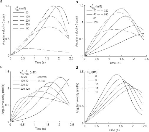
Predicted angular velocity versus time with different initial conditions. (a) Varying initial intracellular concentration of K⁺; (b) Cl⁻; (c) both K⁺ and Cl⁻; and (d) varying initial radius of the cell R₀.

Effects of initial conditions

The effects of initial conditions, including the ion concentrations c_i⁰, the electrical potential difference across the cell membrane Δψ⁰, and the initial radius of the cell R₀ were also studied within the ranges shown in Table 2. As shown in Fig. 8 a, a rise in the initial intracellular concentration $c_{K_i}^0$ of K⁺ from 50 to 100 mM, while keeping the concentration $c_{C{l}_i}^0$ of Cl⁻ constant, shifts the $\dot{\theta }\left(t\right)$ curve leftward and further rise causes flattening of the curve with a similar upward slope as in Fig. 7, a and b. The curve for $c_{K_i}^0=1000$ mM clearly shows that the peak value in $\dot{\theta }$ would be reached at shorter times for higher $c_{K_i}^0$. For the effects of $c_{C{l}_i}^0$ shown in Fig. 8 b, a rise in $c_{C{l}_i}^0$ would first make the curve sharper and narrower as is similar to Fig. 7, c–e, but further rise in $c_{C{l}_i}^0$ would flatten the curve as is similar to Fig. 8 a. In contrast, if $c_{K_i}^0$ and $c_{C{l}_i}^0$ are increased simultaneously by the same ratio (Fig. 8 c), the curve would have a steeper upward slope and a lower peak.

Table 2.

Range of initial variables used in the model

Symbol of the variables [unit]	Range	Value for the trials of other variables
$C_{K_{in}}^0$ [mol]a	50–1000	200
$C_{C{l}_{in}}^0$ [mol]b	80–640	80
Δψ0 [V]c	0.14–0.04	0.14
R0 [μm]d	8–12	1

The first and second columns are the symbol and the range of the variable. The last column for each variable is the value used for the trials of other variables.

^aInitial intracellular concentration of K⁺.

^bInitial intracellular concentration of Cl⁻.

^cInitial electrical potential difference across cell membrane.

^dInitial radius of the cell.

The flatter dashed curves in Fig. 8, a and b, are due to the coupled flow of K⁺ and Cl⁻. When this happens, the change of concentration of the ions is limited by the species with the lower initial concentration difference. Moreover, a higher initial ion concentration difference would lead to a higher initial rate of change of ΔΠ as implied by Eqs. A7 and A8. Therefore, the $\dot{\theta }\left(t\right)$ curve would have a similarly steep upward slope once $c_{K_i}^0$ or $c_{C{l}_i}^0$ exceeds a limit; and, although the initial osmotic and hydrostatic pressure difference would be higher, the change in ion concentration would always be similar due to the limitation. Therefore, the three pressure terms in Eq. A7 could balance each other more quickly, leading to the peak in a shorter time. In contrast to Fig. 8, a and b, the curves in Fig. 8 c do not have the limit and the curves become steeper initially under the increase.

Lastly, a higher initial cell radius R₀ as shown in Fig. 8 d would change the $\dot{\theta }\left(t\right)$ curve in the similar way as increasing L_w in Fig. 7 c, because a smaller R₀ would lead to a higher E′ and smaller R′ in Eqs. A4 and A7. This produces two effects, one similar to an increase in E or v, and another similar to an increase in ΔΠ₀. The first effect will shift the peak to the left and make the curve flatter, whereas the second effect will cause a higher initial slope and higher peak value as in the solid curves in Fig. 8 b. The combined effects lead to the curves in Fig. 8 d.

To summarize, the response of the angular velocity to variations of the material constants and initial conditions includes a change in the peak value and the upward and downward slopes. As R, θ, and Δc_i are coupled, the response is diverse but a general trend for the effects of different variables could be obtained, which is useful for the curve-fitting in the next section.

It is also worthwhile to point out that a decrease in Δψ₀ by 0.1–1.0 V was found to produce no apparent effect on the angular velocity. Such a decrease would represent the necessary change in the membrane potential to open the voltage-gated ion channels in the model, which is the difference between the threshold membrane potential for the activation of the outward K⁺ current (∼−0.050 V according to Stoeckel and Takeda (20)), and the reversal potential (∼−0.14 V). The change in Δψ₀, with or without increasing D_i to D^′_i, in Eq. A8, would only lead to a small difference in Δψ by ∼1 × 10⁻⁷ V within 1 ms and so it can only produce a very slight influence on the angular velocity. Therefore, of the two possible causes of the seismonastic stimulation discussed beforehand, the opening up of the ion channels (the ϕ_i effect) is much more important than the cell depolarization effect (the Δψ effect). Fig. 7 e in fact shows that the movement velocity of the pulvinus changes significantly with the value of ϕ_i.

Comparison of predicted angular velocity with experimental results

The above investigations show that a large range of angular velocity of petiole can be obtained depending on the choice of the material constants and initial conditions. When fitting the model predictions to the experimental results, the focus was put on L_w and ϕ_i for the following reasons. As shown in Figs. 7 b and 8 d, the effects of v and R₀ are smaller within their reasonable ranges. As for E, although its range is larger, its effect is not significant when it is small enough as shown in Fig. 7 a. Because the highest values of the experimentally measured angular velocity in Fig. 2 are ∼1 rad/s, E could not be much larger than 1 MPa for reasonable choice of other variables. Also, as D_i and ϕ_i produce similar results, D_i can be fixed and assigned the largest value found in the literature so as to find out the optimum ϕ_i from the curve-fitting.

In Fig. 2, an upper and lower bound are plotted on top of the experimental results. The values of the parameters are L_w = 2.5 × 10⁻¹¹ ms⁻¹ Pa⁻¹; $c_{K_i}^0=250$ mM; $c_{C{l}_i}^0=100$ mM; ϕ_i = 11 and 13 m s⁻¹; and E = 3.5 and 7.0 MPa for upper and lower bounds, respectively. The remaining constants are given in the last column of Tables 1 and 2. The results reveal that an increase of <15 times in D_i is sufficient to produce the observed movement. As mentioned above, an increase in D_i alone can produce the triggering effect, whereas depolarization, represented by a decrease in Δψ, would cause very minor effects in the prediction. Therefore, the major reason for the triggering of water and ion fluxes should be the opening of the ion channels.

Comparison of predicted volumetric strain of the cell with experimental results

The predicted volumetric strain corresponding to the model curves in Fig. 2 was calculated to be ∼−40 and −45% for the lower and upper bounds, corresponding to ∼−16 and ∼−18% strain in the radius, respectively, showing an agreeable order of magnitude albeit a small underestimation when compared to the −20 to −38% obtained in the experiment. The underestimation is possibly due to the approximations in the model. The most relevant one is that the cells may deform mainly in the longitudinal direction of the pulvinus in reality, whereas the cell in the model deforms uniformly, leading to an underestimation on the strain of the radius. Other factors such as the neglect of intracellular structure, impermeable ions, and the coupling effect of extensor and flexor cells may further lower the predicted results.

Despite the approximations, our model can successfully predict the general trend of angular velocity versus time within the correct order of magnitude as illustrated in Fig. 2. Because the main assumption involved in the model is the water redistribution mechanism, our results show that this mechanism is a possible mechanism for the seismonastic movement.

Conclusions

An ion-water transport model yields values of the angular velocity of petiole and volumetric strain of extensor cells, which are in good agreement with experimental measurements, thus validating the water redistribution mechanism of seismonastic movement. The water and ion fluxes in the mechanism are likely to be caused by the opening of ion channels in the motor cell membranes upon stimulation. The validation of the mechanism may shed light on the development of a new type of intelligent material that can respond to electrical or mechanical stimuli.

Appendix

In the governing equation (Eq. 3) for the volume flow of the model, ΔΠ is given by

$$\Delta \Pi =\overline{R}T\sum _i{\sigma }_i\Delta c_i,$$ (A1)

where ${\sigma }_i=1-\omega \overline{v_i}/L_w$ with $\overline{v_i}$ being the partial molar volume of the ion species i, which is very close to unity for both K⁺ and Cl⁻ and so taken as 1, and $\Delta c_i=c_{i_o}-c_{i_i}$ is the concentration difference of the ion. For ΔP, the dynamic pressure profile inside and outside the cell can be found by the Navier-Stokes equation for inviscid, incompressible flow with spherical symmetry,

$$-\frac{\partial P}{\partial r}=\rho \left(\frac{\partial u}{\partial t}+u\frac{\partial u}{\partial r}\right),$$ (A2)

where u(r, t) is the water velocity field and ρ is the water density. Continuity requires that

$$r\frac{\partial u}{\partial r}+2u=0,$$

which gives u(r, t) = A(t)/r². However, at r → 0 for the cell, u must be finite because there is no source or sink placed at the center of the cell, hence A(t) ≡ 0, and u(r, t) ≡ 0. As a result, from Eq. A2, P does not depend on r whether inside or outside the cell. Thus, ΔP becomes the hydrostatic pressure difference across the cell membrane, given by

$$\Delta P=\frac{-2\gamma }{R}-P_w,$$ (A3)

with γ being the line tension of the cell wall and P_w the pressure caused by the weight of the petiole that the cell is supporting.

The surface tension is related to the hoop stress of the cell wall by the assumption that the cell wall is a homogeneous and isotropic elastic material (Assumption 1; see main text). Using a plane stress stress-strain relation in a polar coordinate, 2γ/R can be expressed in terms of R by

$$\frac{2\gamma }{R}=\frac{E^{\prime }\left(R^3-R^{\prime 3}\right)}{R},$$ (A4)

where E′ = 2tE[3R′³(1 − v)]⁻¹ with t and R′ being the thickness of cell wall and a reference radius of the cell at zero surface tension, respectively, and E and v being the elastic modulus and the Poisson’s ratio of the cell wall, respectively. At the initial condition before the plant is triggered, the surface tension γ₀ is not zero due to the petiole’s weight and the initial osmotic pressure, and the reference radius R′ is determined by the condition that the initial pressure terms are balanced, i.e.,

$$\frac{2{\gamma }_0}{R_0}=\frac{E^{\prime }\left(R_0^3-R^{\prime 3}\right)}{R_0}=-P_{w_0}-\Delta {\Pi }_0,$$

in which rearranging gives

$$R^{\prime 3}=R_0^3{\left[1-\frac{3R_0\left(1-v\right)}{2tE}\left(P_{w_0}+\Delta {\Pi }_0\right)\right]}^{-1},$$ (A5)

where R₀ is the initial radius of the cell. As for P_w, the bending stress equation for simple bending gives

$$P_w=\frac{My}{I},$$ (A6)

with M = mgl_m being the moment exerted by the weight of the petiole on the pulvinus, y the distance of the cell from the neutral axis (see Fig. 5), and I the moment of area of the cylindrical pulvinus. The mass of the petiole m is ∼0.5 g and the moment arm l_m can be taken as the length of the petiole (5 cm) × sinθ, where θ is the angle of the petiole from the pulvinus as shown in Fig. 1. The variable y is chosen to be 1 mm, which is the radius of the cross section of the pulvinus and therefore I = π(0.001)⁴/4 m⁴.

Water flow J_w and the coefficient of hydraulic permeability L_w are used instead of J_v and L_p in Eq. 3 because the volume of the ions is small compared to water, and so the total flow is identified with the water flow. J_w is positive if water flows out of the cell. As stated in Assumption 4 (see main text), the volume of the cell is assumed to be equal to the water volume, and so for a spherical cell,

$$J_w=\frac{-\left(4\pi R^2\dot{R}\right)}{\left(4\pi R^2\right)}=-\dot{R}.$$

With Eqs. A1, A3, A4, and A6, Eq. 3 becomes

$$\dot{R}=-L_w\left[\overline{R}T\sum _i{\sigma }_i\Delta c_i+E^{\prime }\left(\frac{R^3-R^{\prime 3}}{R}\right)+\frac{My}{l}\right],$$ (A7)

which is an expanded version of Eq. 4.

Next, the governing equation for the ion flow across the cell membrane J_i [mol m⁻² s⁻¹] is given by a sum of the reduced form of the Nernst-Planck equation and a constant active flux J_i^A,

$$J_i=-D_i\left(\Delta c_i+\alpha \overline{c_i}\Delta \psi \right)+J_i^A,$$ (A8)

where D_i [m s⁻¹] is the diffusive coefficient of the ion across the cell membrane, which equals $\omega \overline{R}T$ when compared to Eq. 2, and $\alpha =z_{i}F/\left(\overline{R}T\right)$ with z_i being the valence of the ion species i, F being the Faraday constant (96,485 C mol⁻¹), $\overline{c_i}=\left(c_{i_o}+c_{i_i}\right)/2$ is the mean value of the ion concentration, and Δψ is the electrical potential difference across the membrane. The value Δψ is obtained by considering the cell membrane as a capacitor, namely,

$$\Delta \psi =\frac{zF}{3C^{\prime }}R\left(\sum _i{z}_i\Delta c_i+\Delta c_f\right),$$ (A9)

where C′ is the capacitance of the cell membrane, which has a typical value 0.01 Fm⁻² (29), z_iΔc_i is the valence (z_i) × difference of the concentration of the ion species (c_i) across the cell membrane, and Δc_f is the difference of the fixed charge concentration, which can be calculated by the initial conditions Δψ₀, $\Delta c_K^0$, and $\Delta c_{Cl}^0$. The active flux of ions J_i^A is assumed to be constant as not much information on the modeling of the active transport in M. pudica is available. J_i^A can be calculated using the initial condition that the net flux of each ion is zero, i.e., $J_i^A=D_i{\left(\Delta c_i+\alpha \overline{c_i}\Delta \psi \right)}_{t=0}$.

The last governing equation is for the mass conservation of the ions,

$$\begin{array}{c}{c}_{i_i}=\frac{3}{4\pi R^3}\left[\frac{4\pi R_0^3}{3}{c}_{i_i}^0-\underset{0}{\overset{t}{\int }}{J}_i\left(\tau \right)4\pi R^2\left(\tau \right)d\tau \right]\\ c_{i_o}=c_{i_o}^0\end{array},$$ (A10)

where R₀ is the initial radius of the cell and $c_{i_i}^0$ is the initial intracellular concentration of ion i. The extracellular ion concentration $c_{i_o}$ is assumed to be a constant (Assumption 3). The initial extracellular concentration of K⁺ $\left(c_{K_i}\right)$ and Cl⁻ $\left(c_{C{l}_i}\right)$ are chosen as 25 and 10 mM to match the reported values mentioned above.

Equations A8–A10, together with Eq. 5, were solved numerically using an explicit method. As the ions do not contribute to the total volume, the radius R was constant when computing $c_{i_i}$ in Eq. A10. Once $c_{i_i}$ was computed, Eq. A10 was solved by the explicit Euler’s method. The time step was chosen to be small (2 × 10⁻⁶ s) so as to improve the accuracy of the result, especially when the coupled Eqs. A8 and A9 were solved separately.

References

- 1.Sibaoka T. Rapid plant movements triggered by action potentials. Botan. M. 1991;104:73–95. [Google Scholar]
- 2.Weintraub M. Leaf movements in Mimosa pudica L. New Phytol. 1952;50:357–382. [Google Scholar]
- 3.Volkov A.G., Foster J.C., Markin V.S. Mimosa pudica: electrical and mechanical stimulation of plant movements. Plant Cell Environ. 2010;33:163–173. doi: 10.1111/j.1365-3040.2009.02066.x. [DOI] [PubMed] [Google Scholar]
- 4.Kanzawa N., Hoshino Y., Tsuchiya T. Change in the actin cytoskeleton during seismonastic movement of Mimosa pudica. Plant Cell Physiol. 2006;47:531–539. doi: 10.1093/pcp/pcj022. [DOI] [PubMed] [Google Scholar]
- 5.Ueda M., Yamamura S. The chemistry of leaf-movement in Mimosa pudica L. Tetrahedron. 1999;55:10937–10948. [Google Scholar]
- 6.Fratzl P., Barth F.G. Biomaterial systems for mechanosensing and actuation. Nature. 2009;462:442–448. doi: 10.1038/nature08603. [DOI] [PubMed] [Google Scholar]
- 7.Taya M. Bio-inspired design of intelligent materials, Smart Structures and Materials 2003: Electroactive Polymer Actuators and Devices. Proc. SPIE. 2003;5051:45–65. [Google Scholar]
- 8.Singh A.V., Rahman A., Parazzoli D. Bio-inspired approaches to design smart fabrics. Mater. Des. 2012;36:829–839. [Google Scholar]
- 9.Garcia-Cordova F., Valero L., Otero T.F. Biomimetic polypyrrole based all three-in-one triple layer sensing actuators exchanging cations. J. Mater. Chem. 2011;21:17265–17272. [Google Scholar]
- 10.Choe K., Kim K.J. Polyacrylonitrile linear actuators: chemomechanical and electro-chemomechanical properties. Sens. Actuators A Phys. 2006;126:165–172. [Google Scholar]
- 11.Volkov A.G., Foster J.C., Markin V.S. Mechanical and electrical anisotropy in Mimosa pudica pulvini. Plant Signal. Behav. 2010;5:1211–1221. doi: 10.4161/psb.5.10.12658. [DOI] [PMC free article] [PubMed] [Google Scholar]
- 12.Tamiya T., Miyazaki T., Tsuchiya T. Movement of water in conjunction with plant movement visualized by NMR imaging. J. Biochem. 1988;104:5–8. doi: 10.1093/oxfordjournals.jbchem.a122421. [DOI] [PubMed] [Google Scholar]
- 13.Pfeffer G.J. Pfeffer’s plant physiology. Am. Nat. 1905;39:53–55. [Google Scholar]
- 14.Ricca U. Solution of a problem of physiology: the propagation of stimulus in Mimosa [Soluzione d’un problema di fisiologia: la propagazione di stimolo nella Mimosa] Nuovo Giorn. Bot. Ital. 1916;23:51–170. [Google Scholar]
- 15.Schildknecht H., Bender W. A new phytohormone from Mimosa pudica L. Angew. Chem. Int. Ed. Engl. 1983;22:617. [Google Scholar]
- 16.Allen R.D. Mechanism of the seismonastic reaction in Mimosa pudica. Plant Physiol. 1969;44:1101–1107. doi: 10.1104/pp.44.8.1101. [DOI] [PMC free article] [PubMed] [Google Scholar]
- 17.Kumon K., Tsurumi S. Ion efflux from pulvinar cells during slow downward movement of the petiole of Mimosa pudica L. Induced by photostimulation. J. Plant Physiol. 1984;115:439–443. doi: 10.1016/S0176-1617(84)80043-7. [DOI] [PubMed] [Google Scholar]
- 18.Samejima M., Sibaoka T. Changes in the extracellular ion concentration in the main pulvinus of Mimosa pudica during rapid movement and recovery. Plant Cell Physiol. 1980;21:467–479. [Google Scholar]
- 19.Roblin G., Fleurat-Lessard P. Redistribution of potassium, chloride and calcium during the gravitropically induced movement of Mimosa pudica pulvinus. Planta. 1987;170:242–248. doi: 10.1007/BF00397894. [DOI] [PubMed] [Google Scholar]
- 20.Stoeckel H., Takeda K. Plasmalemmal, voltage-dependent ionic currents from excitable pulvinar motor cells of Mimosa pudica. J. Membr. Biol. 1993;131:179–192. doi: 10.1007/BF02260107. [DOI] [PubMed] [Google Scholar]
- 21.Markin V.S., Volkov A.G., Jovanov E. Active movements in plants: mechanism of trap closure by Dionaea muscipula Ellis. Plant Signal. Behav. 2008;3:778–783. doi: 10.4161/psb.3.10.6041. [DOI] [PMC free article] [PubMed] [Google Scholar]
- 22.Fleurat-Lessard P., Frangne N., Martinoia E. Increased expression of vacuolar aquaporin and H+-ATPase related to motor cell function in Mimosa pudica L. Plant Physiol. 1997;114:827–834. doi: 10.1104/pp.114.3.827. [DOI] [PMC free article] [PubMed] [Google Scholar]
- 23.Toriyama H., Jaffe M.J. Migration of calcium and its role in the regulation of seismonasticity in the motor cell of Mimosa pudica L. Plant Physiol. 1972;49:72–81. doi: 10.1104/pp.49.1.72. [DOI] [PMC free article] [PubMed] [Google Scholar]
- 24.Hong Y., Takano M., Chua N.-H. Expression of three members of the calcium-dependent protein kinase gene family in Arabidopsis thaliana. Plant Mol. Biol. 1996;30:1259–1275. doi: 10.1007/BF00019557. [DOI] [PubMed] [Google Scholar]
- 25.Abe T., Oda K. Resting and action potentials of excitable cells in the main pulvinus of Mimosa pudica. Plant Cell Physiol. 1976;17:1343–1350. [Google Scholar]
- 26.Fleurat-Lessard P., Bouche-Pillon S., Bonnemain J.L. Distribution and activity of the plasma membrane H+-ATPase in Mimosa pudica L. in relation to ionic fluxes and leaf movements. Plant Physiol. 1997;113:747–754. doi: 10.1104/pp.113.3.747. [DOI] [PMC free article] [PubMed] [Google Scholar]
- 27.Sibaoka T. Excitable cells in Mimosa. Science. 1962;137:226–227. doi: 10.1126/science.137.3525.226. [DOI] [PubMed] [Google Scholar]
- 28.Kedem O., Katchalsky A. Thermodynamic analysis of the permeability of biological membranes to non-electrolytes. Biochim. Biophys. Acta. 1958;27:229–246. doi: 10.1016/0006-3002(58)90330-5. [DOI] [PubMed] [Google Scholar]
- 29.Nobel P.S. Physicochemical and Environmental Plant Physiology, 4th Ed. Academic Press; San Diego, CA: 2009. Solutes. [Google Scholar]
- 30.Gibson L.J. The hierarchical structure and mechanics of plant materials. J. Roy. Soc. Interface. 2012;9:749–2766. doi: 10.1098/rsif.2012.0341. [DOI] [PMC free article] [PubMed] [Google Scholar]
- 31.Maurel C. Aquaporins and water permeability of plant membranes. Annu. Rev. Plant Physiol. Plant Mol. Biol. 1997;48:399–429. doi: 10.1146/annurev.arplant.48.1.399. [DOI] [PubMed] [Google Scholar]
- 32.Atwell B.J., Kriedemann P.E., Turnbull C.G.N. MacMillan Education Australia; South Melbourne, Australia: 1999. Plants in Action: Adaptation in Nature, Performance in Cultivation. [Google Scholar]