Image reconstruction for sparse-view CT and interior CT—introduction to compressed sensing and differentiated backprojection

Abstract

New designs of future computed tomography (CT) scanners called sparse-view CT and interior CT have been considered in the CT community. Since these CTs measure only incomplete projection data, a key to put these CT scanners to practical use is a development of advanced image reconstruction methods. After 2000, there was a large progress in this research area briefly summarized as follows. In the sparse-view CT, various image reconstruction methods using the compressed sensing (CS) framework have been developed towards reconstructing clinically feasible images from a reduced number of projection data. In the interior CT, several novel theoretical results on solution uniqueness and solution stability have been obtained thanks to the discovery of a new class of reconstruction methods called differentiated backprojection (DBP). In this paper, we mainly review this progress including mathematical principles of the CS image reconstruction and the DBP image reconstruction for readers unfamiliar with this area. We also show some experimental results from our past research to demonstrate that this progress is not only theoretically elegant but also works in practical imaging situations.

Introduction

Computed tomography (CT) is one of important imaging modalities for medical diagnosis. With respect to designs of CT scanners, there was a remarkable progress after 1990. In particular, 3D multi-detector CT scanners and 4D CT scanners have been developed, which dramatically changed the way of medical diagnosis. In this paper, we deal with an active direction of research in the CT community concerning three new designs of CT scanners called sparse-view CT, interior CT, and low-dose CT. The sparse-view CT refers to CT in which measured number of projection data is reduced to less than 100 determined by applications and required image quality. The reduction of projection data leads to benefits such as reducing patient dose, reducing scan time, and improving time-resolution in cardiac CT. The interior CT refers to CT in which X-ray beam is radiated only to a small region of interest (ROI) such as heart or breast determined from the disease to be diagnosed. It has been demonstrated that the interior CT leads to various benefits such as reducing patient dose outside the ROI and reducing necessary detector size. The low-dose CT refers to CT in which power of X-ray tube is decreased to reduce patient dose. Since it became apparent that the cancer risk increases by excessive CT examinations, the low-dose CT has been considered an important research topic in the CT community.

To put these new CT scanners to practical use for medical diagnosis, a development of advanced image reconstruction methods is required, because all of these CTs measure only incomplete projection data so that classical image reconstruction methods such as filtered backprojection (FBP) and algebraic reconstruction technique (ART) are not successful in producing clinically feasible images. Therefore, the development of image reconstruction methods for the sparse-view CT, the interior CT, and the low-dose CT is an area of active research since 2000 and a remarkable progress has been made. In this paper, we review the progress of such image reconstruction research for unfamiliar readers. Due to the lack of space, we limit the target to the sparse-view CT and the interior CT. A nice review of techniques for the low-dose CT can be found in (1,2). Also, a review covering wider topics on newest image reconstruction research was written by the experts in this field (3).

Sparse-view CT and image reconstruction

What is sparse-view CT?

The principle of sparse-view CT is shown in Figure 1. In the ordinary fan-beam CT, projection data is measured from 1,000-2,000 X-ray source positions uniformly distributed over the angular range 0≤θ<2π. In the sparse-view CT, the number of projection data is reduced to less than 100 determined by applications and required image quality. Below, we summarize major benefits obtained by reducing the number of projection data.

Figure 1.

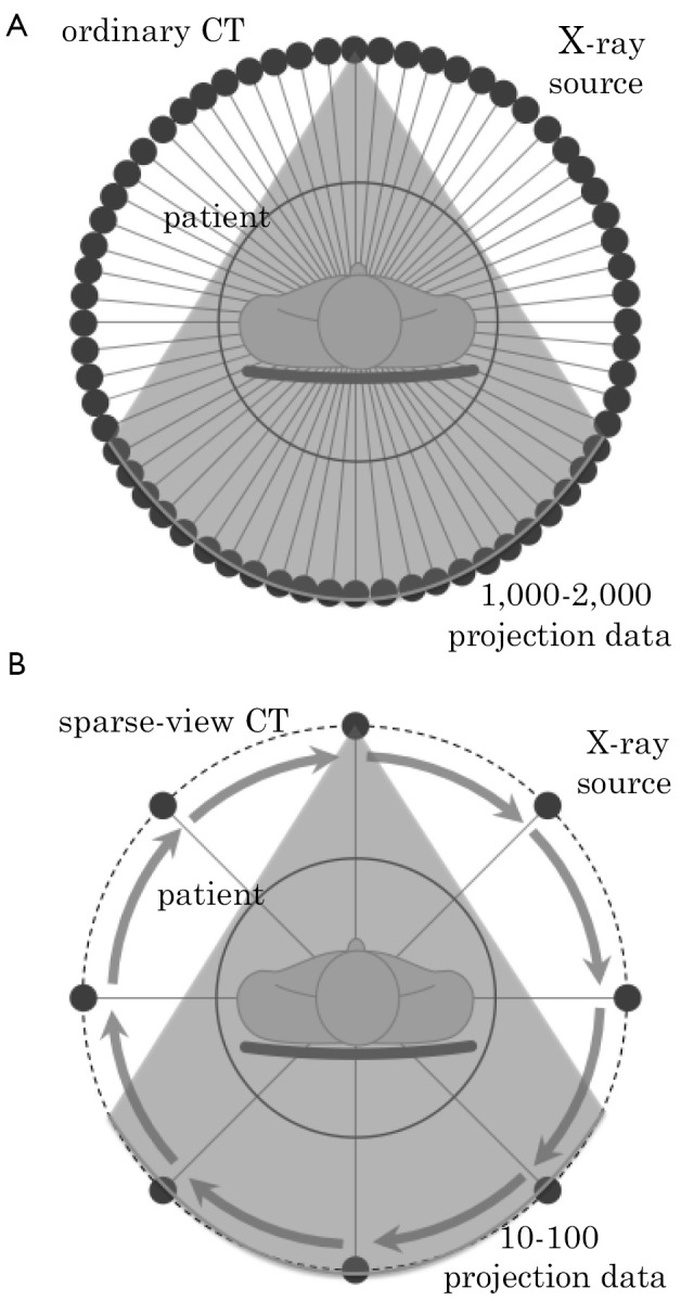
Schematic illustration of data acquisition in (A) the ordinary CT and (B) the sparse-view CT. In the sparse-view CT, the number of measured projection data is reduced to less than 100 determined by applications and required image quality

Micro CT, flat panel detector CT, and 3D angiography

In micro CT used for small animal imaging and non-destructive testing, X-ray exposure time per each projection data is longer compared to that in commercial medical CT scanners. Furthermore, time to transfer the measured projection data to a computer requires a large time. These situations are very similar in low-cost CT using a flat panel detector and 3D angiography. Therefore, reducing the number of projection data possesses a significant benefit in these equipments.

Reducing patient dose

In commercial CT scanners, reducing the number of projection data contributes to reducing patient dose. As an alternative strategy to reduce the patient dose, we can also consider to reduce X-ray tube power while measuring the sufficient number of projection data. At the current stage, it is not very clear which method outperforms the other.

Cardiac imaging

In cardiac CT, so-called cardiac gating is used to decrease motion artifacts. The principle is outlined as follows. The projection data is measured over many n heart beats by continuously rotating an X-ray source together with a measurement of electrocardiogram. To reconstruct an image at each time phase t, the projection data measured at similar time phase is picked up from all the projection data and is used for reconstruction. A comprehensive review of cardiac CT imaging can be found in (4,5). However, when the measurement time period n is not sufficiently large to reduce patient dose or to shorten examination time, we cannot pick up the large number of projection data anymore for each time phase t so that the image reconstruction must be performed from the small number of projection data.

Compressed sensing image reconstruction

Next, we explain image reconstruction methods from a small number of projection data. First, we explain solution uniqueness of this reconstruction problem. Old works in the mathematical literature demonstrate that the solution to image reconstruction from a finite number of projection data is not unique (6,7). Therefore, to achieve satisfactory reconstructions, some prior knowledge on the object to be imaged must be employed. Classically, many researchers investigated this problem with a variety of reconstruction methods and prior knowledge (8,9). A nice review concerning this research area before 1990 can be found in (10), but no one has found an excellent method which can be used in practice. The situation has changed dramatically during 2000’s thanks to the discovery of so-called compressed sensing (CS) as a new technique to solve inverse problems. The goal of CS is to reconstruct a signal or an image from measured sensor data undersampled below the Nyquist rate violating the conditions of Shannon sampling theorem. The pioneering papers of CS were written by Donoho (11) and by Candes et al. (12).

We introduce the mathematical principle of CS as comprehensive as possible. The problem treated in the CS is formulated as follows. We represent the original image to be reconstructed and the measured projection data by

[1]

where J is the number of pixels and I is the number of sampling points in the projection data. We represent the system matrix relating and by A={a_ij}. Using these definitions, we have the measurement equation

[2]

Then, our problem is to recover from when I<J. We note that equation [2] is an underdetermined linear equation having infinite solutions given . The principle of CS can be roughly described as follows. The key is a concept called “sparsity”. We assume that the vector obtained by applying some transform W, called sparsifying transform, to is sparse in the sense that most components of are close to zeros, i.e., negligibly small. By using this property, we can reduce the number of unknowns in equation [2] from J to I so that equation [2] is uniquely solvable achieving accurate image reconstruction. The selection of sparsifying transform W is important in the CS. For example, the identity operator can be used for blood-vessel images and star images obtained by a telescope, because these images themselves are sparse. For general images, we can use the gradient operator or the wavelet transform as a sparsifying transform, because derivative signals are expected to become sparse in most parts except for highly active parts such as edges and textures.

Next, we explain detailed methods of image recovery. In the CS, we are required to perform the following two tasks, i.e., (I) identifying negligible components of and (II) recovering by assuming that the negligible components of are zeros. Normally, the following clever framework using a nice property of L₁, L₀ norms is used to perform the two tasks simultaneously. We begin by defining the cost function of image reconstruction by

[3]

where W is the K×J matrix representing the sparsifying transform and is the reference image closer to the object , i.e., is sparse. The role of W and is to convert into a sparse vector as much as possible. Concrete choices of W and for a variety of imaging situations can be found in the literature (13-37). In equation [3], the parameter 0≤p≤2 is the order of norm. In classical solution techniques of inverse problems, p=2 is normally used. On the other hand, to evaluate the degree of sparsity in a more rigorous way, p=1 or 0 is used in the CS, where

[4]

The norm corresponding to p=1 (or 0) is called the L₁ (or L₀) norm. The L₀ norm can be interpreted as the number of non-zero components of a vector, and the L₁ norm is a convex function which approximates the L₀ norm well. In Figure 2, to understand why the L₁, L₀ norms pick up the sparse solutions better compared to the standard L₂ norm, we show equi-contour lines of the L₂, L₁, L₀ norms for the case where is a 2D vector. It is observed that the L₁, L₀ norms yield larger costs to non-sparse vectors, which are located far from the coordinate axes, compared to the L₂ norm. This property, often called “L₁, L₀ magic”, is the key, which explains why the L₁, L₀ norms possess a significantly stronger power in picking up the sparse solutions. Using equation [3] as the cost function to pick up a reasonable sparse solution, we formulate the image reconstruction problem as the following linearly constrained minimization.

Figure 2.

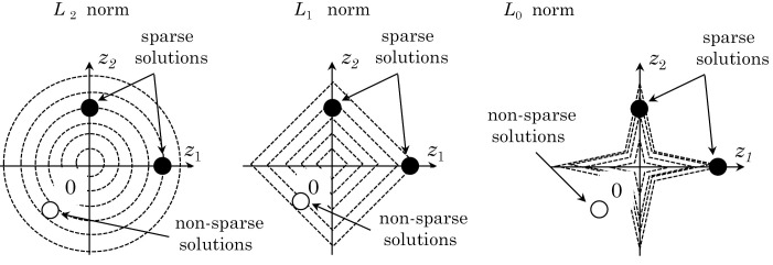
Equi-contour lines corresponding to the L₂, L₁, L₀ norm cost functions in the case where is a 2D vector. The L₁, L₀ norms have a property that they yield larger costs to non-sparse points located far from the coordinate axes, which leads to a strong power in picking up sparse solutions better than the L₂ norm

[5]

The CS was originally proposed to solve the signal reconstruction from the undersampled data. However, the same approach can be used to solve denoising problems and image reconstructions from noisy projection data. In these cases, under the assumption that the additive noise is Gaussian, the problem is formulated as the following unconstrained minimization.

[6]

As a special case of the CS, the total variation (TV) minimization is frequently used for image reconstruction in the sparse-view CT, which is also called “ROF model” because it was first proposed by Rudin, Osher, and Fatemi (14). In the TV minimization, the cost function is defined by

[7]

where i_mn is a gray-scale value of the image at the pixel (m,n). The meaning of equation [7] can be interpreted as the L₁ norm of the magnitude image of intensity gradient .

Next, we explain iterative methods to solve the problems formulated by equations [5] and [6]. First, the problems in equations [5] and [6] cannot be solved by using classical differentiable optimization techniques such as the gradient method, because the L₁, L₀ norms are neither strictly convex nor differentiable. Therefore, in the CS field, a development of valid iterative methods to solve the L₁, L₀ norm minimization is an area of active research. A nice review of this area can be found in (15-18). Among many famous methods, the iterative-thresholding (IT) method has been used in many cases (19). Since the constrained problem of equation [5] can be reformulated in the form of equation [6] using the penalty method, we describe the IT method to solve the unconstrained problem [6]. For simplicity, the explanation below assumes that the sparsifying transform W is the orthogonal J×J matrix and the reference image is zero. The IT method is derived based on the majorization-minimization (MM) technique, which is known to be a powerful and general tool to develop a wider class of iterative methods (20,21). Denoting the iteration number by k, the structure of algorithm construction in the MM technique is summarized as follows.

[Step 1] (Majorization) At the current iterate , construct a surrogate function satisfying the following conditions.

[8]

[Step 2] (Minimization) Minimize instead of to obtain the next iterate .

We note that the MM technique can be thought of as a method to replace the minimization of complex cost function into a sequence of tractable minimizations of . If is constructed such that equation [8] is satisfied, the iteration is convergent. Furthermore, if the original cost and the surrogate function satisfy some additional assumptions [such as the convexity of ] (20,21), the sequence converges to the solution to the original problem. In our current problem of the CS, can be constructed in the following way.

[9]

where α>||A^T A|| is a constant and we replaced A^T A by αI to derive the last inequality. Simplifying equation [9] by putting the terms independent of into the constant C yields

[10]

We note that can be considered an image obtained by applying one iteration of the gradient descent with the least-squares term to . This observation allows us to summarize the IT method as follows.

[Step 1] (Initialization) Set the initial image . Set the iteration number as k←0.

[Step 2] (Computation of intermediate image) Compute the intermediate image from the current iterate by second equation of [10].

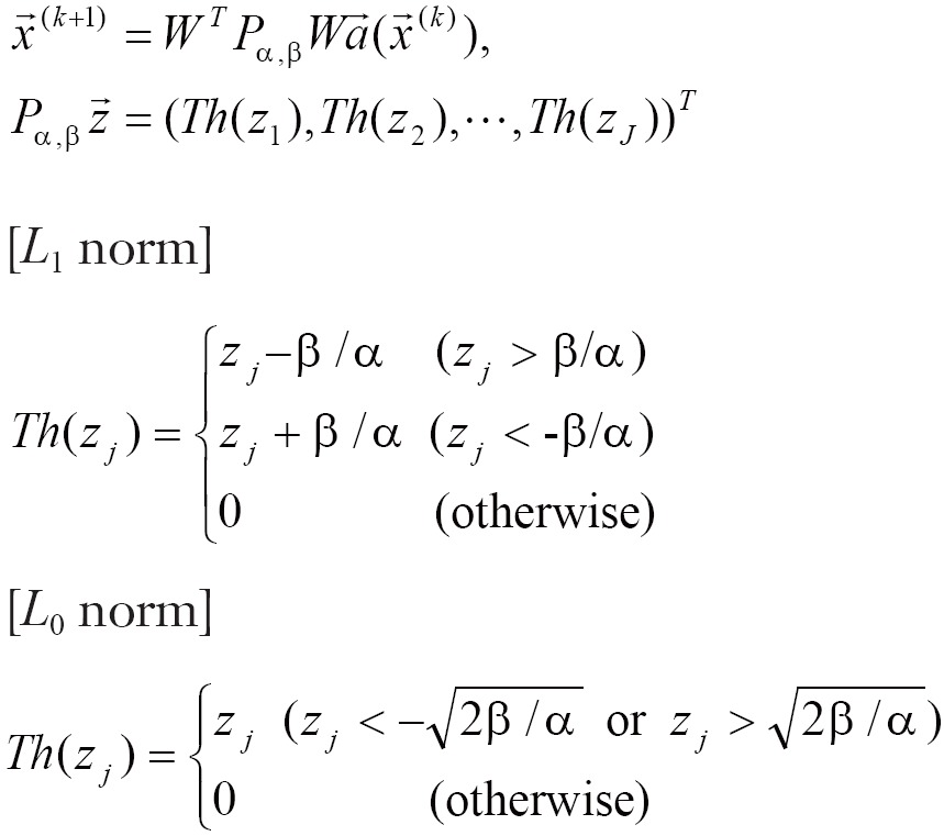
[Step 3] (Minimization of surrogate function) Minimize , i.e., first equation of [10], to obtain the next iterate . This minimization can be done in closed form when is the L₁ norm or the L₀ norm (19), the result of which is expressed as

[11]

[Step 4] Increase the iteration number as k←k+1. Go to [Step 2].

The operation appearing in [Step 3] can be interpreted as a kind of thresholding in the space of sparsified data as follows. First, we apply the forward transform W to to obtain the transformed vector . Next, we apply the thresholding operation expressed by Th(z_j) in equation [11] to each component z_j. Finally, we apply the inverse transform W^T to come back to the original space. In Figure 3, we show input-output functions corresponding to this thresholding operation for the L₁, L₀ norms. The left one corresponding to the L₁ norm is called “soft thresholding”, which cuts all small components to zeros and decrease large components towards zeros. On the other hand, the right one corresponding to the L₀ norm is called “hard thresholding”, which cuts all small components to zeros and keep large components with no change. Finally, we would like to strengthen that the above derivation leads to an algorithm which repeats (I) the gradient descent update using the least-squares term and (II) the thresholding operation in the transformed space alternately. The name “iterative thresholding” originates from this algorithmic structure. Its convergence to the solution to the problem [6] is proved for the case of L₁ norm. The convergence in the case of L₀ norm is unknown mainly due to the non-convex nature of the cost function. Finally, we would like to mention that the IT method can be also viewed as an application of the forward backward splitting method to solve the non-linear monotone equation, and, in this case, the thresholding operator P_α,β corresponds to the proximal operator (18).

Figure 3.

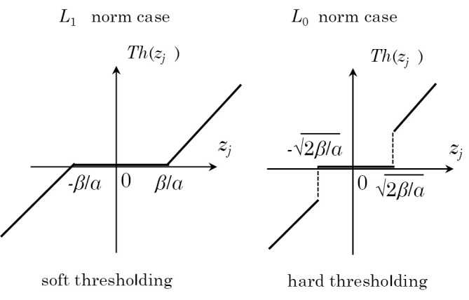
Thresholding operations in implementing the iterative—thresholding method corresponding to the L₁, L₀ norms

Overview of existing research

As we mentioned earlier, Donoho and Candes et al. proposed the concept of CS in the middle of 2000’s (11,12). Before and after these publications, too many authors have applied the CS to image reconstruction for the sparse-view CT. We cannot review all the activities due to the lack of space. Therefore, we mainly introduce works done in the early stage. To the best of our knowledge, the first paper which applied the CS to tomography was published by Li et al. (22). They applied the CS to reconstruct a sparse blood-vessel image from few projection data measured with contrast agent using the L₁ norm cost function. In Figure 4, we show their reconstructed images in comparison to those obtained by the classical ART method. It is known that the ART iteration converges to a solution minimizing the L₂ norm when applied to the underdetermined linear equation. Therefore, this result demonstrates that the difference between the L₁ norm and the L₂ norm in the task of recovering a sparse image is surprisingly larger than what we imagine intuitively. Another earlier work was done by Sidky et al. (23,24). They applied the TV minimization to a variety of image reconstruction problems with incomplete projection data. They also developed a number of different iterative methods for the TV minimization, in which the overall structure is to repeat one iteration of the ART method and updating the image towards the descent direction of TV alternately (they named “ART-TV”). Other works on the use of TV can be also found in (25,26). One more important work in the early stage was done by Chen et al. (27,28). They developed a reconstruction method called Prior Image Constrained Compressed Sensing (PICCS) for cardiac CT and other applications. The PICCS method uses the cost function similar to that in equation [3], i.e., a reference image together with the gradient operator as a sparsifying transform. In the case of cardiac CT, the reference image can be constructed from the other neighboring time frames or by averaging all the frames. We also mention that the CS has become popular in MRI reconstruction (29). Very Recently, Rashed and Kudo developed an alternative method called intensity MAP (I-MAP) reconstruction, in which only information of intensity histogram expressed in the form of Laplacian mixture model is used instead of the reference image as prior knowledge (30). All the above-mentioned papers showed surprising reconstructed images.

Figure 4.

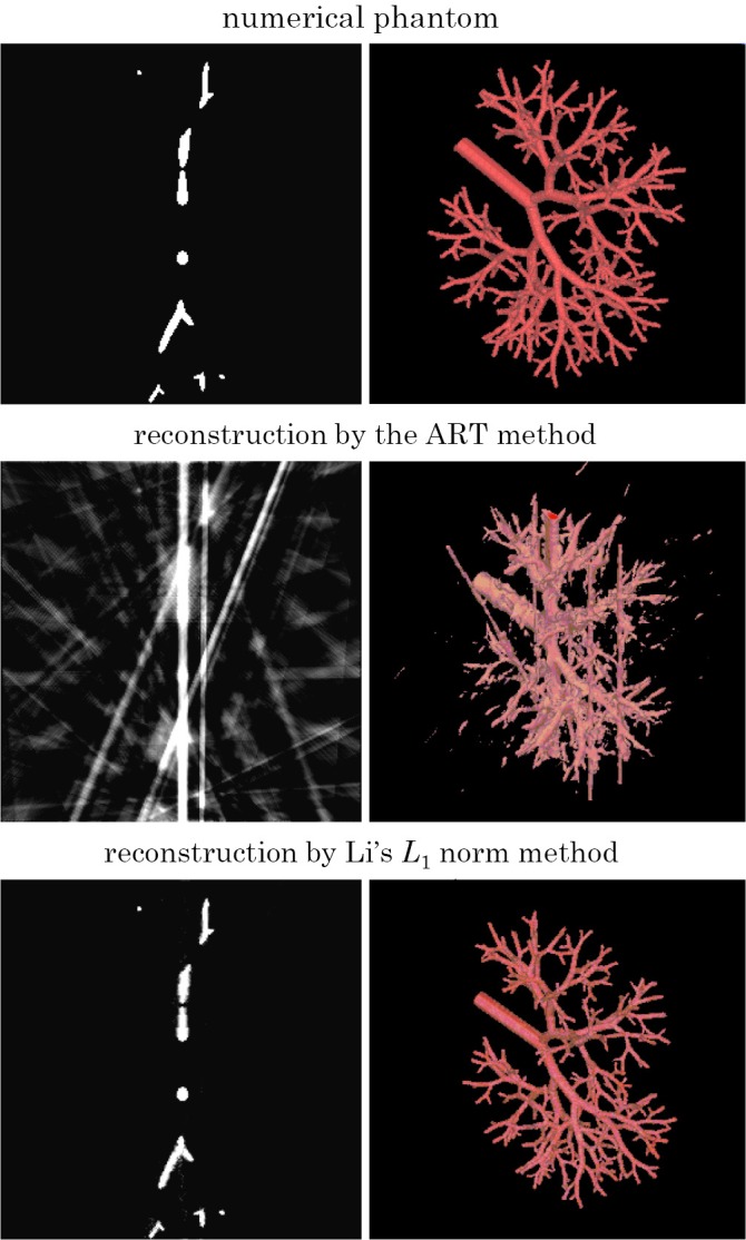
Reconstructions of sparse blood-vessel images by the ART method and Li’s L₁ norm method (22). We note that the ART method is an iterative method which uses the L₂ norm cost function. It is observed that the L₁ norm cost function has a strong power in picking up sparse solutions well

On the other hand, Herman and Davidi claimed that “exact” reconstructions from a small number of projection data are impossible due to the existence of null space of the operator, and “what we can do best” is to improve the degraded images (31). They showed an example in which the TV minimization fails. Similarly to their explanation, in Figure 5, we show a trivial example of the existence of null space. In this figure, we assume that projection data are measured from two directions, i.e., horizontal and vertical. Then, the projection data of the left image coincides with that of the right image. The TV minimization favors the left image than the right image, because the length of region boundaries for the left is shorter than the right. Therefore, the structure of central lesion part of the right image disappears by the TV minimization.

Figure 5.

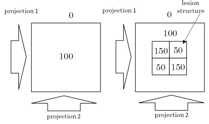
Illustration of the existence of null space for image reconstruction from two projections. Projection data are measured from two directions, i.e., horizontal and vertical. Since the projection data of the left image coincides with that of the right image, the TV minimization favors the left image having shorter region boundaries than the right image. Therefore, the central lesion structure in the right object disappears by the TV minimization

Some recent trend is to develop a class of iterative methods, which can treat the non-smoothness of TV in a rigorous way using techniques of convex optimization and non-linear variational analysis. We note that the IT method cannot be used for the TV minimization because the differentiation operator associated with the TV in equation [7] is not a pure orthogonal transform but a tight frame. For example, works along this direction were published by Defrise et al. (using the MM technique) (32), Ramani and Fessler (using the alternating direction method of multipliers, ADMM) (33), and Sidky and Pan (using the Chambolle-Pock primal-dual algorithm) (34). An alternative future direction would be to employ past CT images of the same or other persons in the form of prior knowledge to improve the reconstructions. For example, Xu et al. (35), Van de Sompel et al. (36), and Rashed and Kudo (37) investigated such approaches.

We show our non-published simulation results for chest CT imaging. In this study, a numerical phantom simulating a human chest slice was reconstructed from only 16 projection data. We developed a reconstruction method which uses the TV cost function combined with the constrained formulation of equation [5]. We show reconstructed images in Figure 6 together with reconstructions by the classical ART and FBP methods. As shown in many other papers too, it is observed that streak artifacts arising due the angular undersampling are almost perfectly eliminated while fine structures inside the lung are preserved well.

Figure 6.

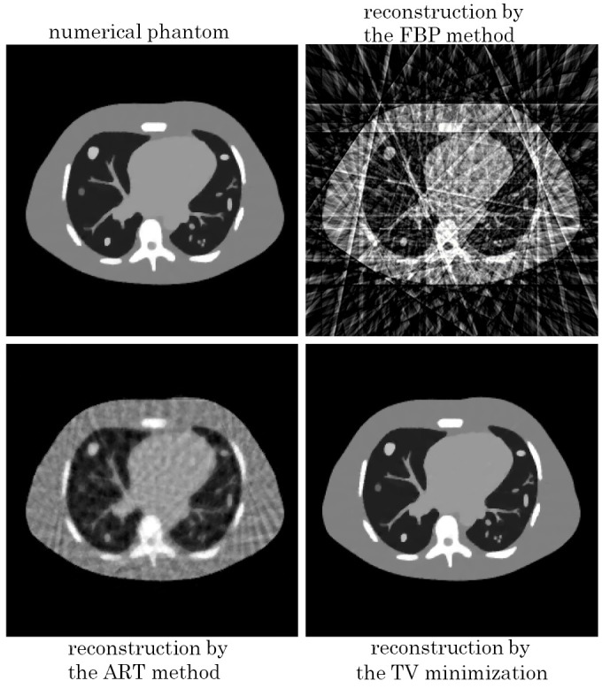
Reconstructions from 16 projection data of the chest numerical phantom by using the FBP method, the ART method, and the TV minimization. It is observed that the TV minimization eliminates streak artifacts almost perfectly while preserves fine structures inside the lung well

Interior CT and image reconstruction

What is interior CT?

The principle of interior CT is shown in Figure 7 in comparison to the geometry of ordinary CT. In many situations of medical diagnosis, physicians are interested in a relatively small ROI containing a target of diagnosis. For example, such situations occur in cardiac imaging, mammography, and abdominal imaging to examine some specific single organ. In these cases, current CT scanners still need to measure complete projection data covering the whole object which corresponds to all lines passing through the whole object (not only the ROI). However, it can be intuitively expected that the projection data passing through the ROI (red line in Figure 7B) cannot be reduced, but the projection data passing through only outside the ROI (blue line in Figure 7B) need not be measured because they do not bring information inside the ROI. Based on this observation, the interior CT refers to new CT in which only a set of projection data passing through the ROI is measured. Potential impacts of the interior CT in clinical diagnosis are not clear at the current stage, but we expect that it lead to the following advantages over the conventional CT.

Figure 7.

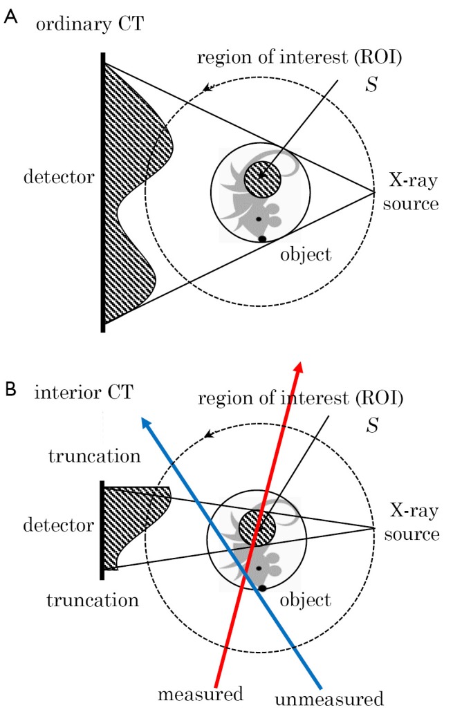
Schematic illustration of data acquisition in (A) the ordinary CT and (B) the interior CT. In the interior CT, an X-ray beam from each source position covers only a small ROI containing a target of diagnosis. For example, projection data corresponding to the red line is measured, but projection data corresponding to the blue line is unmeasured

Reducing patient dose

Even in the interior CT, patient dose inside the ROI cannot be reduced. However, the dose outside the ROI can be significantly reduced. We have done some Monte Carlo simulation study evaluating the patient dose outside the ROI for the case of cardiac imaging. The result demonstrates that the dose can be reduced to approximately 20-30 percent of that of the conventional CT. Of course, the degree of achieved dose reduction depends on the ratio of the size of ROI to the size of whole object.

Imaging a large object extending outside scanner field of view

In many instances of medical or non-destructive testing CT applications, it is required to reconstruct a partial ROI of a large object extending outside the scanner field of view (FOV). For example, hands sometimes extend beyond the FOV in medical CT. These cases cannot be exactly handled in the conventional CT.

Reducing detector size and X-ray beam width

Similarly, the interior CT also leads to reducing necessary detector size and X-ray beam width when imaging a partial ROI. For example, this advantage is significant in the synchrotron radiation CT in which available X-ray beam is very narrow (38).

Major theoretical advances

Next, we review theoretical advances of image reconstruction for the interior CT which occurred mainly after 2004. We begin by formulating the reconstruction problem in the interior CT. As shown in Figure 8, we represent the object by a function f(x,y) and represent the convex ROI to be imaged by S. For simplicity, we consider the parallel-beam geometry and represent the projection data by a function p(r,ϕ), where r is the radial variable and ϕ is the angle. Extending the explanation below to the case of fan-beam geometry is easy. In the interior CT, we measure all values of p(r,ϕ) corresponding to a set of lines passing through the ROI S, and do not measure p(r,ϕ) corresponding to a set of lines not passing through the ROI S at all. Consequently, the projection data p(r,ϕ) corresponding to each angle ϕ is truncated at least either in the left or right part dependent on the size and the location of ROI S. Image reconstruction from such truncated projection data is called “ROI reconstruction” or “interior reconstruction”.

Figure 8.

Three different situations of the ROI reconstruction. A. The case treated by Noo et al. (39) and Pan et al. (40); B. the case treated by Defrise et al. (41); C. the case of interior problem (42-44)

Up to 2004, approximate reconstructions based on various iterative reconstruction methods or extrapolating the truncated part of p(r,ϕ) by a smooth function followed by the FBP reconstruction had been investigated in many papers (45,46). On the other hand, after Noo et al. (39) and Pan et al. (40) independently discovered a new analytical reconstruction method called differentiated backprojection (DBP) which possesses a potential to exactly solve the ROI reconstruction, several authors demonstrated that the solution to the ROI reconstruction is determined in the “unique” and “stable” way under the assumptions that (I) the size and the location of ROI S satisfy some geometrical condition and (II) some prior knowledge on the object f(x,y) is available (41-44,47-54). Here, the word “unique” refers to the fact that the solution to the problem is uniquely determined, and the word “stable” refers to the fact that the inversion is stable in the sense that perturbations (such as noise and discretization errors) on the measured data or the prior knowledge are not amplified during the inversion. Also, we note that the word “prior knowledge” implies that the function f(x,y) is known on some specified region inside or outside the ROI S. Due to the lack of space, we cannot explain all the research activities along this direction. Therefore, as a useful index for unfamiliar readers to search for the corresponding original papers, in Table 1, we summarize theoretical results concerning the uniqueness and the stability discovered after 2004. Most these results have been obtained based on the above-mentioned DBP concept. First, in the papers of Noo et al. (39) and Pan et al. (40), they proved that the ROI reconstruction can be uniquely and stably solved if the ROI S is a convex region containing both the left and right boundaries of the object (Figure 8A). In 2006, Defrise et al. (41) investigated the case where the ROI S is a convex region containing only one of the left or right boundaries of the object (Figure 8B). By using the fact that there exists a small region B located outside the object and inside the ROI S in which we know that f(x,y)=0, they proved that the solution is still unique and obtained some stability estimate demonstrating that the inversion is only “mildly ill-posed”. The left problem at this stage is the case where the ROI S is a convex region completely contained inside the object f(x,y) corresponding to the setup of interior CT (Figure 8C). For this case, some mathematical literature had already proved that the solution to the ROI reconstruction is not unique such that there exists a non-trivial null space (48,49). On the other hand, by using the DBP concept, Ye et al. (42) and Kudo et al. (43,44) independently proved that the interior problem can be uniquely solved and the inversion is “mildly ill-posed” if we know the object f(x,y) on a small region B located inside the ROI S. The surprising fact is that the prior knowledge region B assuring the solution uniqueness can be an arbitrary small region having non-zero measure (single point is not enough). Kudo et al. expressed this fact by the phrase “Tiny a priori knowledge solves the interior problem”.

Table 1. Summary of various uniqueness results obtained in the research of interior CT.

Year	Reference	ROI S	Reconstructed region	Prior knowledge	Solution stability
2004	Noo (39)	Figure 8A	ROI S	No B	Stable
2005	Pan (40)
2006	Defrise (41)	Figure 8B	ROI S	Object support B	Mildly ill-posed
2007	Ye (42)	Figure 8C	ROI S	Region B	Mildly ill-posed
2008	Kudo (43)
2008	Courdurier (44)
2008	Ye (50)	Figure 8C	Whole object	Region B	Severely ill-posed
2008	Courdurier (44)
2009	Li (51)	Figure 8B+8C	ROI S	Object support B	Unknown
2008	Yu (52)	Figure 8C	Whole object	Piecewise constant object	Unknown
2009	Van Gompel (53)	Figure 8C	Whole object	Single object with constant intensity	Mildly ill-posed
2013	Wang (54)	Figure 8C	ROI S	Partial region outside ROI S (E-line)	Mildly ill-posed

Other new uniqueness results can be found in Ye et al. (50), Courdurier et al. (44), Li et al. (51), Yu and Wang (52), Van Gompel et al. (53), and Wang and Kudo (54). In particular, Yu and Wang proved that the solution for the setup of interior CT (Figure 8C) is unique on both inside and outside the ROI if we know that the object f(x,y) is a piecewise constant function everywhere and proposed a reconstruction method using the TV minimization (52).

Differentiated backprojection method

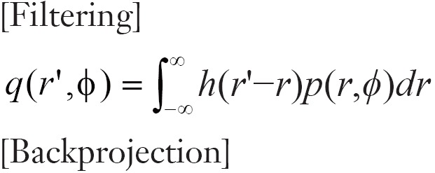
Next, we explain the DBP reconstruction method in some rigorous way such that unfamiliar readers can understand why this method contributes to exactly solving the ROI reconstruction. First, we begin by explaining why the classical FBP method cannot solve the ROI reconstruction. The procedure of FBP reconstruction for the parallel-beam geometry is expressed as the following two steps.

[12]

[13]

where h(·) is the kernel of ramp filter applied to the projection data p(r,ϕ). It is well-known that h(·) is a function having infinite support (extending to infinity) so that the filtering operation [12] is non-local. Therefore, the computation of filtering by equation [12] involves all values of p(r,ϕ) even if we only need partial filtered data q(r,ϕ) backprojected to the small ROI S. To overcome this drawback, in the papers of Noo et al. (39) and Pan et al. (40), they divided the ramp filtering into a succession of the differentiation and the Hilbert transform, and exchanged the order of the Hilbert transform and the backprojection.

The resulting DBP method is summarized in the following form. The key is to decompose the ROI S into a set of straight lines L(u);uϵU called Hilbert line (u is the parameter to specify each line), and to factorize the 2-D reconstruction problem into the inverse Hilbert transform along each Hilbert line. First, in prior to the reconstruction, we decompose the ROI S into a set of Hilbert lines L(u);uϵU such that the following two conditions are satisfied.

(I) Each point (x,y) belongs to at least one lines L(u);

(II) In the setup of Figure 8B,C, all the lines L(u) intersect the prior knowledge region B.

In Figure 9, we illustrate typical decompositions corresponding to each setup shown in Figure 8. After performing this decomposition, the DBP method reconstructs f(x,y) on each Hilbert line L(u) in a line-by-line manner according to the following steps.

Figure 9.

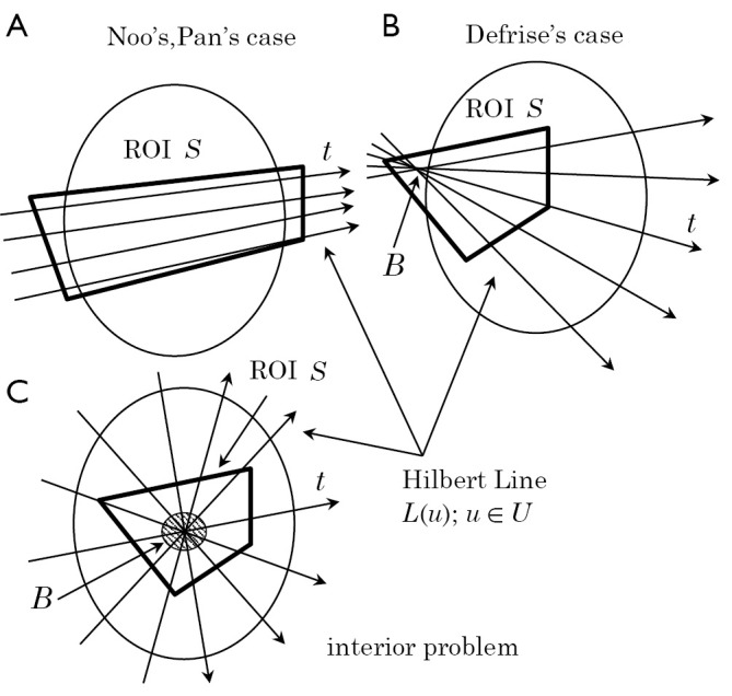
Example choices of a set of valid Hilbert lines corresponding to each situation shown in Figure 8

[Step 1] (DBP) For all (x,y)ϵS∩L(u), we compute the DBP by the following equation to obtain an intermediate image g(u,x,y) called Hilbert image.

[14]

where θ(u) is the angle between L(u) and the x-axis. We note that the DBP cannot be computed outside S∩L(u) due to the lack of P(r,ϕ) over ϕϵ[0,π).

[Step 2] (Hilbert inverse) On each Hilbert line L(u), we define the coordinate t as shown in Figure 8 where the coordinate origin can be arbitrary. We denote f(x,y) and g(u,x,y) on the t-axis by functions f(t) and g(t) respectively. Then, the relation between f(t) and g(t) can be expressed by the Hilbert transform as

[15]

where p.v denotes the Cauchy principal value of integral and the definition of points (a,b,c,d,e,f) are shown in Figure 8 dependent on each case. Therefore, the image reconstruction on the Hilbert line L(u) can be reduced to the inversion of Hilbert transform. The inversion for each case of Figure 8 can be performed as follows.

(I) Case of Figure 8A

In this case, we have (b,e)⊃(a,f) and equation [15] is called the finite Hilbert transform. The following inversion formula of finite Hilbert transform is available to perform the inversion (47).

[16]

We can compute equation [16] because C is the projection data along the Hilbert line L(u), which is measured.

(II) Case of Figures 8B,C

In these cases, the main feature is that the Hilbert transform g(t) is available only on the limited interval (b,e) which does not cover the whole object support (a,f), i.e., (b,e)⊂(a,f). In other words, the Hilbert transform is truncated. Such Hilbert transform is called truncated Hilbert transform (41). It is known that the solution to equation [15] is not unique for any point tϵ(a,f). However, let us remind that we can use the prior knowledge of f(t) on the interval tϵ(c,d) which corresponds to the prior knowledge interval L(u)∩B. By using analyticity of the Hilbert transform kernel, it was proved that the combination of equation [15] and this prior knowledge uniquely determines f(t) on the interval (b,e) which corresponds to the whole ROI interval L(u)∩S (41-44,50). Unfortunately, analytical inversion formulae are not available. Defrise et al. (41), Ye et al. (42), and Kudo et al. (43,44) used the iterative method called Projection Onto Convex Set (POCS) to perform this inversion.

Example reconstructed images

We show two example reconstructed images in the interior CT from our past research. The first example is the reconstruction of head CT projection data shown in Kudo et al. (43). As shown in Figure 10, we considered the setup where the ROI S is a rectangular region located inside the head and the prior knowledge region B is the strip region located at the left end of S. We compared the reconstructed image with the prior knowledge and that without the prior knowledge. The result clearly demonstrates that the small prior knowledge significantly reduces the low-frequency shading artifact occurring due to the non-uniqueness of solution in the interior CT. The second example in Figure 11 shows reconstructions of pulmonary alveoli of a small mouse and a phantom consisting of calcite in talc powder. These objects were imaged using the synchrotron radiation CT at SPring-8 facility in Japan. In the both objects, there exist air regions inside the object on which we know that the value of attenuation coefficient is zero. The air regions were automatically identified using a special iterative method using the L₁ norm minimization described in Rashed and Kudo (38), which were used as the prior knowledge region B for reconstruction. Similarly to the case of head CT, the strong shading artifacts occurring at the boundaries were almost perfectly eliminated by using the prior knowledge.

Figure 10.

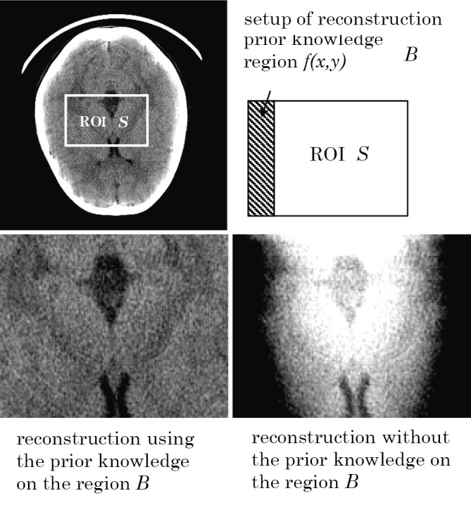
Reconstructions of real CT data for head imaging where the ROI S is a rectangular region located inside the head. We compared the reconstruction by using the prior knowledge of object in the region B (located at the left end of ROI S) to the reconstruction without the prior knowledge. The result demonstrates that the very small prior knowledge dramatically reduces the low-frequency shading artifacts.

Figure 11.

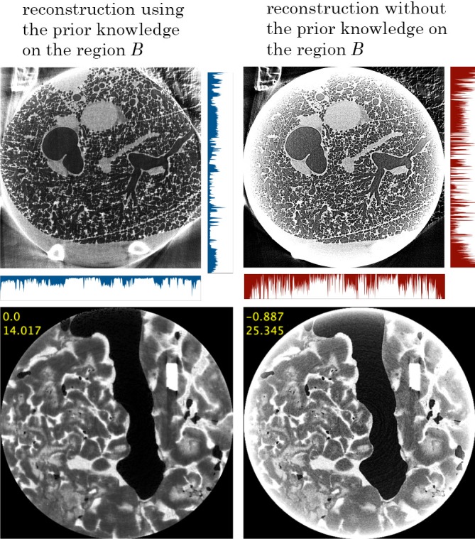
Reconstructed images of real projection data obtained by the synchrotron radiation CT at the SPring-8 facility in Japan. The top row shows reconstructions of pulmonary alveoli of a mouse lung, and the bottom row shows reconstructions of a phantom consisting of calcite in talc powder. In the both cases, we identified air regions using the iterative method proposed by Rashed and Kudo (38), which were used as the prior knowledge region B. It is observed that the low-frequency shading artifacts at the boundaries of the ROI significantly reduce by using the prior knowledge

Overview of related research

Several authors extended the DBP approach to other imaging geometries such as cone-beam CT (55-57), single-photon emission CT (58,59), cardiac CT (60), and phase-contrast CT (61). In particular, Pan et al. (55), Noo et al. (56), and Ye et al. (57) extended the DBP method to cone-beam CT. Unfortunately, the resulting DBP method still requires a complicated implementation mainly due to the lack of freedom in the choice of Hilbert lines (called PI lines in the cone-beam geometry) so that further research is necessary for its practical use. Furthermore, a case study of how to acquire the prior knowledge to assure the solution uniqueness in actual imaging situations has been investigated (62). Another direction is to use various iterative reconstruction methods including those belonging to the CS framework for the interior CT instead of the DBP method (38,52,59,63).

Finally, we would like to mention that Clackdoyle et al. (64) discovered an alternative approach, called “virtual fan-beam method”, to solve the ROI reconstruction in 2004. An interesting observation is that this method leads to a data sufficiency condition for exact ROI reconstruction which is different from that of the DBP concept.

Conclusions

This paper picked up two relatively large topics, sparse-view CT and interior CT, both of which are under investigation in the CT community. We explained their recent advances mainly from the image reconstruction perspective. In the sparse-view CT, image reconstruction based on the CS has been the major promising research direction after 2000. In the interior CT, after 2004, there have been significant progresses in theoretical parts concerning the solution uniqueness and the solution stability.

References

- 1.Rampinelli C, Origgi D, Bellomi M.Low-dose CT: technique, reading methods and image interpretation. Cancer Imaging 2013;12:548-56 [DOI] [PMC free article] [PubMed] [Google Scholar]
- 2.Kubo T, Lin PJ, Stiller W, et al. Radiation dose reduction in chest CT: a review. AJR Am J Roentgenol 2008;190:335-43 [DOI] [PubMed] [Google Scholar]
- 3.Pan X, Sidky EY, Vannier M. Why do commercial CT scanners still employ traditional, filtered back-projection for image reconstruction? Inverse Probl 2009;25:1230009. [DOI] [PMC free article] [PubMed] [Google Scholar]
- 4.Bonnet S, Koenig A, Roux S, et al. Dynamic x-ray computed tomography. Proc IEEE 2003;91:1574-87 [Google Scholar]
- 5.Hsieh J. Computed tomography: principles, design, artifacts, and recent advances (2nd ed). SPIE Press, 2009. [Google Scholar]
- 6.Smith KT, Solmon DC, Wagner SL. Practical and mathematical aspects of the problem of reconstructing objects from radiographs. Bull Amer Math Soc 1977;83:1227-70 [Google Scholar]
- 7.Louis AK. Ghosts in tomography - The null space of the Radon transform. Math Methods Appl Sci 1981;3:1-10 [Google Scholar]
- 8.Llacer J.Theory of imaging with a very limited number of projections. IEEE Trans Nucl Sci 1979;NS-26:596-602 [Google Scholar]
- 9.Siltanen S, Kolehmainen V, Järvenpää S, et al. Statistical inversion for medical x-ray tomography with few radiographs: I. General theory. Phys Med Biol 2003;48:1437-63 [DOI] [PubMed] [Google Scholar]
- 10.Rangayyan R, Dhawan AP, Gordon R. Algorithms for limited-view computed tomography: an annotated bibliography and a challenge. Appl Opt 1985;24:4000-12 [DOI] [PubMed] [Google Scholar]
- 11.Donoho DL. Compressed sensing. IEEE Trans Inf Theory 2006;52:1289-306 [Google Scholar]
- 12.Candès EJ, Romberg J, Tao T. Robust uncertainty principles: exact signal reconstruction from highly incomplete frequency information. IEEE Trans Inf Theory 2006;52:489-509 [Google Scholar]
- 13.Candes EJ, Wakin MB. An introduction to compressive sampling. IEEE Signal Processing Magazine 2008;25:21-30 [Google Scholar]
- 14.Rudin LI, Osher S, Fatemi E. Nonlinear total variation noise removal algorithm. Physica D 1992;60:259-68 [Google Scholar]
- 15.Eldar YC, Kutyniok G. Compressed sensing: theory and applications. Cambridge University Press, 2012. [Google Scholar]
- 16.Starck JL, Murtagh F, Fadili JM. Sparse image and signal processing: wavelets, curvelets, morphological diversity. Cambridge University Press 2010. [Google Scholar]
- 17.Elad M. Sparse and redundant representations: from theory to applications in signal and image processing. Springer, 2010. [Google Scholar]
- 18.Combettes PL, Pesquet JC. Proximal splitting methods in signal processing (in Fixed-point algorithms for inverse problems in science and engineering. Springer 2011:185-212).
- 19.Daubechies I, Defrise M, DeMol C.An iterative thresholding algorithm for linear inverse problms with a sparsity constraint. Comm Pure Appl Math 2004;57:1413-57 [Google Scholar]
- 20.Lange K. Optimization (2nd ed). Springer, 2013. [Google Scholar]
- 21.Lange K, Hunter DR, Yang I. Optimization transfer using surrogate objective functions. J Comput Graph Stat 2000;9:1-20 [Google Scholar]
- 22.Li M, Yang H, Kudo H.An accurate iterative reconstruction algorithm for sparse objects: application to 3D blood vessel reconstruction from a limited number of projections. Phys Med Biol 2002;47:2599-609 [DOI] [PubMed] [Google Scholar]
- 23.Sidky EY, Kao CM, Pan X. Accurate image reconstruction from few-views and limited-angle data in divergent-beam CT. J X-ray Sci Tech 2006;14:119-39 [Google Scholar]
- 24.Sidky EY, Pan X. Image reconstruction in circular cone-beam computed tomography by constrained, total-variation minimization. Phys Med Biol 2008;53:4777-807 [DOI] [PMC free article] [PubMed] [Google Scholar]
- 25.Song J, Liu QH, Johnson GA, et al. Sparseness prior based iterative image reconstruction for retrospectively gated cardiac micro-CT. Med Phys 2007;34:4476-83 [DOI] [PMC free article] [PubMed] [Google Scholar]
- 26.Ritschl L, Bergner F, Fleischmann C, et al. Improved total variation-based CT image reconstruction applied to clinical data. Phys Med Biol 2011;56:1545-61 [DOI] [PubMed] [Google Scholar]
- 27.Chen GH, Tang J, Leng S. Prior image constrained compressed sensing (PICCS): a method to accurately reconstruct dynamic CT images from highly undersampled projection data sets. Med Phys 2008;35:660-3 [DOI] [PMC free article] [PubMed] [Google Scholar]
- 28.Leng S, Tang J, Zambelli J, et al. High temporal resolution and streak-free four-dimensional cone-beam computed tomography. Phys Med Biol 2008;53:5653-73 [DOI] [PMC free article] [PubMed] [Google Scholar]
- 29.Trzasko J, Manduca A.Highly undersampled magnetic resonance image reconstruction via homotopic l(0) -minimization. IEEE Trans Med Imaging 2009;28:106-21 [DOI] [PubMed] [Google Scholar]
- 30.Rashed EA, Kudo H. Statistical image reconstruction from limited projection data with intensity priors. Phys Med Biol 2012;57:2039-61 [DOI] [PubMed] [Google Scholar]
- 31.Herman GT, Davidi R. On image reconstruction from a small number of projections. Inverse Probl 2008;24:45011-28 [DOI] [PMC free article] [PubMed] [Google Scholar]
- 32.Defrise M, Vanhove C, Liu X.An algorithm for total variation regularization in high-dimensional linear problems. Inverse Probl 2011;27:065002 [Google Scholar]
- 33.Ramani S, Fessler JA. A splitting-based iterative algorithm for accelerated statistical X-ray CT reconstruction. IEEE Trans Med Imaging 2012;31:677-88 [DOI] [PMC free article] [PubMed] [Google Scholar]
- 34.Sidky EY, Jørgensen JH, Pan X. Convex optimization problem prototyping for image reconstruction in computed tomography with the Chambolle-Pock algorithm. Phys Med Biol 2012;57:3065-91 [DOI] [PMC free article] [PubMed] [Google Scholar]
- 35.Xu Q, Yu H, Mou X, et al. Low-dose X-ray CT reconstruction via dictionary learning. IEEE Trans Med Imaging 2012;31:1682-97 [DOI] [PMC free article] [PubMed] [Google Scholar]
- 36.Van de Sompel D, Brady M.Regularising limited view tomography using anatomical reference images and information theoretic similarity metrics. Med Image Anal 2012;16:278-300 [DOI] [PubMed] [Google Scholar]
- 37.Rashed EA, Kudo H. Statistical CT reconstruction from limited views with probabilistic atlas prior. Proceedings of the Second International Meeting on Image Formation in X-ray Computed Tomography 2012;352-5. [Google Scholar]
- 38.Rashed EA, Kudo H. Towards high-resolution synchrotron radiation imaging with statistical iterative reconstruction. J Synchrotron Radiat 2013;20:116-24 [DOI] [PubMed] [Google Scholar]
- 39.Noo F, Clackdoyle R, Pack JD. A two-step Hilbert transform method for 2D image reconstruction. Phys Med Biol 2004;49:3903-23 [DOI] [PubMed] [Google Scholar]
- 40.Pan X, Zou Y, Xia D.Image reconstruction in peripheral and central regions-of-interest and data redundancy. Med Phys 2005;32:673-84 [DOI] [PubMed] [Google Scholar]
- 41.Defrise M, Noo F, Clackdoyle R, et al. Truncated Hilbert transform and image reconstruction from limited tomographic data. Inverse Probl 2006;22:1037-53 [Google Scholar]
- 42.Ye Y, Yu H, Wei Y, et al. A general local reconstruction approach based on a truncated hilbert transform. Int J Biomed Imaging 2007;2007:63634. [DOI] [PMC free article] [PubMed]
- 43.Kudo H, Courdurier M, Noo F, et al. Tiny a priori knowledge solves the interior problem in computed tomography. Phys Med Biol 2008;53:2207-31 [DOI] [PubMed] [Google Scholar]
- 44.Courdurier M, Noo F, Defrise M, et al. Solving the interior problem of computed tomography using a priori knowledge. Inverse Probl 2008;24:65001. [DOI] [PMC free article] [PubMed] [Google Scholar]
- 45.Ogawa K, Nakajima M, Yuta S.A reconstruction algorithm from truncated projections. IEEE Trans Med Imaging 1984;3:34-40 [DOI] [PubMed] [Google Scholar]
- 46.Ohnesorge B, Flohr T, Schwarz K, et al. Efficient correction for CT image artifacts caused by objects extending outside the scan field of view. Med Phys 2000;27:39-46 [DOI] [PubMed] [Google Scholar]
- 47.Clackdoyle R, Defrise M.Tomographic reconstruction in the 21st century. IEEE Signal Processing Magazine 2010;27:60-80 [Google Scholar]
- 48.Natterer F. The mathematics of computerized tomography. SIAM 2001. [Google Scholar]
- 49.Maass P.The interior Radon transform. SIAM J Appl Math 1992;52:710-24 [Google Scholar]
- 50.Ye Y, Yu H, Wang G. Exact interior reconstruction from truncated limited-angle projection data. Int J Biomed Imaging 2008;2008:427989. [DOI] [PMC free article] [PubMed]
- 51.Li L, Kang K, Chen Z, et al. A general region-of-interest image reconstruction approach with truncated Hilbert transform. J Xray Sci Technol 2009;17:135-52 [DOI] [PubMed] [Google Scholar]
- 52.Yu H, Wang G.Compressed sensing based interior tomography. Phys Med Biol 2009;54:2791-805 [DOI] [PMC free article] [PubMed] [Google Scholar]
- 53.Van Gompel G, Defrise M, Batenburg KJ. Reconstruction of a uniform star object from interior x-ray data: uniqueness, stability and algorithm. Inverse Probl 2009;25:065010 [Google Scholar]
- 54.Wang Z, Kudo H.Interior reconstruction in computed tomography using a priori knowledge outside the region of interest. Med Imaging Technol 2013;31:113-20 [Google Scholar]
- 55.Zou Y, Pan X.Exact image reconstruction on PI-lines from minimum data in helical cone-beam CT. Phys Med Biol 2004;49:941-59 [DOI] [PubMed] [Google Scholar]
- 56.Pack JD, Noo F, Clackdoyle R. Cone-beam reconstruction using the backprojection of locally filtered projections. IEEE Trans Med Imaging 2005;24:70-85 [DOI] [PubMed] [Google Scholar]
- 57.Ye Y, Zhao S, Yu H, et al. A general exact reconstruction for cone-beam CT via backprojection-filtration. IEEE Trans Med Imaging 2005;24:1190-8 [DOI] [PubMed] [Google Scholar]
- 58.Rullgard H.An explicit inversion formula for the exponential Radon transform using data from 180 degrees. Ark Mat 2004;42:353-62 [Google Scholar]
- 59.Zeng GL, Gullberg GT. SPECT region of interest reconstruction with truncated transmission and emission data. Med Phys 2010;37:4627-33 [DOI] [PMC free article] [PubMed] [Google Scholar]
- 60.Taguchi K, Kudo H.Motion compensated fan-beam reconstruction for nonrigid transformation. IEEE Trans Med Imaging 2008;27:907-17 [DOI] [PubMed] [Google Scholar]
- 61.Lauzier PT, Qi Z, Zambelli J, et al. Interior tomography in x-ray differential phase contrast CT imaging. Phys Med Biol 2012;57:N117-30. [DOI] [PMC free article] [PubMed]
- 62.Bharkhada D, Yu H, Ge S, et al. Cardiac computed tomography radiation dose reduction using interior reconstruction algorithm with the aorta and vertebra as known information. J Comput Assist Tomogr 2009;33:338-47 [DOI] [PMC free article] [PubMed] [Google Scholar]
- 63.Xu Q, Mou X, Wang G, et al. Statistical interior tomography. IEEE Trans Med Imaging 2011;30:1116-28 [DOI] [PMC free article] [PubMed] [Google Scholar]
- 64.Clackdoyle R, Noo F, Guo J, et al. Quantitative reconstruction from truncated projections in classical tomography. IEEE Trans Nucl Sci 2004;51:2570-8 [Google Scholar]