

Abstract
In neurophysiology, extracellular signals—as measured by local field potentials (LFP) or electroencephalography—are of great significance. Their exact biophysical basis is, however, still not fully understood. We present a three-dimensional model exploiting the cylinder symmetry of a single axon in extracellular fluid based on the Poisson-Nernst-Planck equations of electrodiffusion. The propagation of an action potential along the axonal membrane is investigated by means of numerical simulations. Special attention is paid to the Debye layer, the region with strong concentration gradients close to the membrane, which is explicitly resolved by the computational mesh. We focus on the evolution of the extracellular electric potential. A characteristic up-down-up LFP waveform in the far-field is found. Close to the membrane, the potential shows a more intricate shape. A comparison with the widely used line source approximation reveals similarities and demonstrates the strong influence of membrane currents. However, the electrodiffusion model shows another signal component stemming directly from the intracellular electric field, called the action potential echo. Depending on the neuronal configuration, this might have a significant effect on the LFP. In these situations, electrodiffusion models should be used for quantitative comparisons with experimental data.
Introduction
Simulations of neuronal signal propagation have a long history and are well established in neuroscience as a useful tool to study brain function. Most models today are based on the seminal work of Hodgkin and Huxley (1) for the membrane currents and the application of cable theory (2) to account for the neuron morphology. Among the most well-known simulators for these kinds of models are NEURON (3) and GENESIS (4).
Although experimental setups with intracellular recordings can readily be replicated by compartment models, extracellular measurements—an important tool in neurophysiology to study multiunit and network activity—cannot be included directly.
There are models for obtaining the extracellular field of a neuron that are based on the membrane current source density (5,6), based on the line source approximation (LSA) (7), which account for effects like frequency filtering of a complex extracellular space (8,9). In Pettersen et al. (10), an inverse method was applied to estimate current source densities from extracellular potentials. In these models, the relevant parameters for the extracellular medium are conductivity and permittivity. The problem is reduced to the solution of the electrostatic part of Maxwell’s equations, where the membrane is the only current source. The local changes in ion concentrations caused by drift and diffusion and their contribution to the electric field are not considered.
In Lopreore et al. (11), a detailed three-dimensional numerical simulation of electrodiffusion has been carried out for the node of Ranvier, showing the accumulation and depletion of ions close to the membrane, and therefore the invalidity of the electroneutrality approximation close to the membrane, as used in cable equation models. The study focused on deviations from the cable equation, not on the extracellular signal. However, the membrane thickness was greatly overestimated in this study as a consequence of the coarseness of the spatial discretization, presumably dictated by the available computational resources.
In Mori (12), the reason for the high computational demand of electrodiffusion models based on the Poisson-Nernst-Planck (PNP) equations is discussed: The presence of a Debye layer close to the membrane—over which concentrations change significantly—necessitates a fine spatial resolution. A clever approximation is suggested that represents the Debye layer as a charge density boundary condition. In Mori et al. (13), this methodology was applied to study the effect of gap junction conductances on cardiac action potential (AP) propagation.
A recent study (14) investigated the AP propagation in a reconstructed three-dimensional axonal structure intracellularly. Numerical methods for electrodiffusion-reaction equations were analyzed in a comprehensive way in Lu et al. (15), with special regard to surface potentials of biomolecules.
To our knowledge, a model does not yet exist that explicitly resolves the Debye layer to study membrane dynamics following neuronal excitation on the detailed level of electrodiffusion.
In this work, we model the detailed evolution of the concentrations of the most relevant ion species and the resulting electric field inside and (particularly) outside the cell during the spread of an AP along an axonal membrane. To this end, the Poisson-Nernst-Planck equations are solved numerically by application of the finite element method. We propose an efficient numerical scheme to tackle the computational demand by using a suitable spatial grid that resolves the multiple spatial scales accurately while still using only a minimal number of unknowns.
We strive to elucidate how the complex interaction of ion movements explains the evolution of the extracellular signal. Finally, we compare our results with the LSA model and explain the observed differences in signal shape.
Theory and Methods
The Poisson-Nernst-Planck equations of electrodiffusion
The PNP system describes the movement of ions in a static solvent due to diffusion and electrostatic drift. It consists of the Nernst-Planck equation
| (1a) |
with the ion flux
| (1b) |
and the Poisson equation
| (2) |
The ni, i = 1,…, N, are relative concentrations (with respect to a scaling concentration n∗ = NA, equal to the Avogadro constant) with units in millimolar for the N different ion species; zi is the valence; Di is the position-dependent diffusion coefficient of the ion species i; ϕ is the dimensionless relative electric potential energy with respect to the thermal energy (ϕ = eU/kT) with U in volts; for room temperature, ϕ = 1 corresponds to ∼25 mV; ε is the relative permittivity (which again may be position-dependent); and T is the temperature of the solvent.
Equation 1 describes the time-dependent change in concentrations due to diffusion and drift through an electrical field. Equation 2 gives the electric potential ϕ at any point in space. We now use the PNP system to set up a detailed model of an axon in an extracellular medium.
A three-dimensional model of axonal membrane and extracellular space
Our simulation model focuses on the axonal part of the neuron. Here, we are especially interested in the membrane dynamics and its effects on the extracellular signal. As the solution of a full three-dimensional system is computationally expensive, we use a cylindrical coordinate system. Exploiting the rotational symmetry of an idealized axon, the computational domain can be reduced to two dimensions, as there is no change in angular direction. This enables us to calculate valid three-dimensional results with a drastically reduced computational complexity. For the numerical solution, the rectangular elements will be treated as (hollow) cylinders and the volumes calculated accordingly. In the following, the two-dimensional geometry will be used for illustration purposes, while implicitly meaning the cylindrical geometry.
In the upper part of Fig. 1, the cylindrical geometry is shown with the two-dimensional subset highlighted, constituting the effective computational domain. The x axis represents the domain’s symmetry axis, eliminating the angular coordinate θ from the equations. The domain consists of three partitions: Cytosol, membrane, and extracellular space. Cytosol and extracellular space are electrolytes, yielding the electrolyte domain Ωelec. It may contain an arbitrary number N of concentrations of different ion species. Here, however, we will restrict ourselves to the minimal set of N = 3 monovalent species sodium (Na+), potassium (K+), and chloride (Cl−). Sodium and potassium are needed for the ion channel dynamics triggering an action potential; chloride is a representative of the anions needed for electroneutrality in the bulk solution and does not cross the membrane in this model.
Figure 1.

The two-dimensional computational domain for the cylinder symmetric axon model. The upper part shows the cylinder geometry into which the two-dimensional computational grid is embedded, assuming symmetry in the angular direction. (Lower part, solid lines) Domain boundary Γex. (Lower part, dashed lines) Interior (electrolyte-membrane) boundary Γint. This divides the domain into the (unconnected) electrolyte domain and the separating membrane Ωmemb domains. The Debye layer of close to the membrane is highlighted (shading), followed by the near-field and far-field parts. The lower boundary represents the inner-cell symmetry axis. Note that this scheme is not to scale, as the actual mesh sizes in y direction differ by several orders of magnitude between the Debye layer and far-field making the grid very anisotropic.
The membrane domain Ωmemb separates the two parts of the electrolyte domain; therefore, Ωelec is not connected. This setup necessitates the introduction of additional boundary conditions on the membrane-electrolyte-interface Γint next to obligatory boundary conditions on the domain boundary Γext, such that the set of all boundary points is given by Γ = Γint ∩ Γext. The measures Ωelec and Ωmemb form a partition of the computational domain: .
With this multidomain setup, we now have the Nernst-Planck expression from Eq. 1 defined on Ωelec and boundary conditions as
| (3a) |
| (3b) |
and the Poisson expression from Eq. 2 defined on the whole domain Ω with boundary conditions as
| (4a) |
| (4b) |
where n denotes the unit outer normal and Γ⋅,D and Γ⋅,N denote Dirichlet and Neumann boundaries, respectively. For consistency, of course Γext,N ∪ Γext,D = Γext holds.
Equations 1 and 2 are obviously defined on different domains. The Poisson equation is defined on the whole domain, whereas the Nernst-Planck equation is only defined on the electrolyte subdomain. This means we assume the membrane to be free of mobile charge carriers for simplicity. Membrane surface charges could easily be added as an additional source term in the Poisson equation, but are not included here.
As can be seen in Fig. 1, the exterior boundary consists of four parts, and the interior boundary of two nonconnected parts.
For the boundary conditions of Eqs. 3a, 3b, 4a, and 4b, we use
where we call the constant ni0 the bulk concentration of species i. The membrane flux fimemb is defined in the next section. The Dirichlet boundary conditions for the concentrations on the upper exterior boundary serve to model an infinite reservoir for each ion species. The potential is clamped to zero at the upper extracellular boundary, which introduces an error equal to the value of the real potential value calculated for an unrestricted domain (potential is 0 at infinity). For a point charge on the membrane, this error would correspond to an absolute shift at each point in the domain. Because the potential of a point charge falls off as 1/r in three dimensions, increasing the domain size by a factor 100 will reduce the error at a fixed point by a factor 1/100. For a finite line charge (as in our case of an active membrane), this is only true if the radial distance is large compared to the length of the line charge (compare to LSA, e.g., in Gold et al. (5)). In any case, increasing the domain size in the y direction will reduce the error introduced by the upper Dirichlet boundary. We chose a sufficiently large domain size of ymax = 10 mm to account for this.
At the lower boundary representing the intracellular symmetry axis, the potential gradient and ion fluxes are vanishing such that no boundary artifacts are introduced.
Membrane flux
The membrane flux boundary conditions are taken from an effective model of ion channel currents. Given the time- and potential-dependent channel conductances gi(ϕ,t) from the Hodgkin-Huxley scheme (1)—here we use the version from Koch (16), see the Supporting Material for details—the total conductance for each ion species is given by
| (5a) |
| (5b) |
| (5c) |
with voltage-gated conductances , and fixed leak conductances and .
For the definition of the membrane flux, each point x ∈ ΓCYint on the cytosol-membrane interface is mapped to a point μ(x) ∈ ΓESint on the opposite membrane-extracellular space interface by a map μ(x) = x + dmemb ⋅ n, where dmemb is the membrane thickness and n is in this case the unit outer normal at x pointing in the direction from cytosol to membrane. The values of potential and concentrations evaluated at these points are called ϕCY = ϕ(x), niCY = ni(x), ϕES = ϕ(μ(x)), and niES = ni(μ(x)). With these values on both sides of the membrane, the concentration-, potential-, and time-dependent membrane flux fimemb of species i ∈ {Na, K, Cl}is defined as
| (6) |
where [ϕ] denotes the potential jump across the membrane, i.e., [ϕ] = ϕCY − ϕES. Note that two opposite points on the membrane interface are identified with each other here, i.e., the membrane thickness is essentially neglected.
The flux was derived from the Hodgkin-Huxley membrane current Iimemb = gi(ϕ,t)([U] – E) by replacing the constant battery E by a variable concentration-dependent reversal potential calculated from the Nernst equation (see below) and adding necessary scaling factors to bring fimemb = Iimemb/ezn∗ to SI units mol/m2 s. This interior boundary condition fits nicely into our framework, as it unifies the potential-dependent Hodgkin-Huxley system with the concentration-dependent Nernst equation to arrive at an expression that represents all the features of the potential- and concentration-dependent ion flux Fi of the PNP system.
Equilibrium states
The system’s steady state is equivalent to the neuronal resting state. The equilibrium membrane potential can be easily validated: For one ion species, the Nernst equation
| (7) |
gives the potential jump across the membrane.
The Goldman equation usually employed to calculate a neuron’s resting potential is based on the assumption that the two electrolytes separated by the membrane are bulk solutions, i.e., the ion concentrations are constant and only change within the membrane. As our model is based on the opposite assumptions—there are no ions within the membrane, but nonzero ion fluxes in the neighboring electrolytes—the Goldman equation cannot be used to validate the equilibrium state of our model.
The model is initialized by setting the ion concentrations within one electrolyte domain uniformly to their intra- and extracellular bulk values ni0 (see Table S1 in the Supporting Material). The bulk concentrations are chosen such that each electrolyte initially is electroneutral, i.e., the net charge is zero, which is a reasonable assumption both physically and biologically with respect to energy minimization principles.
To generate the resting state, the membrane leak channels are opened. The active channels stay closed during the equilibration phase. After some time (in the range of tens of milliseconds), an equilibrium state will establish with a net zero membrane flux and the concentrations following a Boltzmann distribution.
The Poisson-Boltzmann equation
| (8) |
predicts the concentration profile at equilibrium state. This equation will be used for validation of the simulation later on, it is not explicitly used in the algorithm.
Numerical methods
Finite element discretization
We use a finite element approach using the continuous Galerkin method to solve the equations stated in The Poisson-Nernst-Planck Equations of Electrodiffusion. Multiplying by test functions v, integrating over the domain and applying integration by parts, we obtain the weak formulation of the equations in residual formulation.
For the Nernst-Planck equation, the temporal part
| (9a) |
and the spatial part
| (9b) |
are combined, yielding
| (9c) |
For the Poisson equation, we get
| (10) |
and, therefore, the residual for the full system reads
| (11) |
By applying the method of lines, each equation is discretized in space first by representing the unknown functions ni and ϕ as well as the test functions v by Q1 nodal basis functions on a tensor grid, and then in time using the implicit Euler time-stepping scheme. As suggested in Fig. 1, the grid is refined toward the membrane in the y direction. This is essential to resolve the Debye length, the characteristic length scale over which the electrolyte ion concentrations deviate significantly from their bulk values close to the membrane. In the x direction, the grid is equidistant (dx = 100 μm); in the y direction, it ranges from dymin = 0.5 nm over the Debye layer to dymax = 100 μm, resulting in a very anisotropic grid.
It can easily be seen that each equation alone is linear in its unknowns. One could therefore use an operator-split approach and solve the equations alternately until convergence in each time step. We observed that a very small time step (on the order of nanoseconds) is necessary to solve the system this way.
Because the nonlinearity of the whole system results from the coupling of both equations, it seems reasonable to represent this crucial feature in the numerical method. The system is therefore solved fully coupled using Newton’s method, requiring the solution of one single linear system in each iteration. For small systems, SuperLU (17) was used; for larger systems with >50,000 unknowns, a stabilized BiConjugate Gradient iterative solver, preconditioned by an inexact LU decomposition, turned out to be faster while maintaining the same accuracy. We observe a significantly higher stability leading to possible time steps of approximately tens of microseconds for the fully coupled approach.
The cylinder symmetry introduces another subtle difficulty for the numerical treatment of the system. Because the cell volumes increase in the positive y direction (roughly with y dy), the entries of the full residual R differ by several orders of magnitude (109 for the chosen domain size of 10 mm) solely by the presence of volume integrals in the weak form of the equations. We apply a threshold volume scaling to account for this: At a certain distance from the membrane, a reference volume Vref is calculated. All residuals belonging to an unknown at node i having a volume Vi > Vref, where Vi is the minimum volume of all adjacent cells of node i, are scaled by a factor Vref/Vi. This mathematically corresponds to multiplying a diagonal matrix from left to the linear system matrix, meaning that the same linear system is solved in each Newton iteration. This scaling greatly increases the convergence properties of the Newton algorithm for this cylinder geometry setup.
Adaptive time-stepping
As the system has a great variability during the course of an action potential, a small time step is needed to capture the large fluxes and potential differences during this period. On the other hand, potential differences during interspike intervals are small and so are the magnitudes of ion fluxes, allowing for the use of a larger time step. Therefore, an adaptive time-stepping strategy is used to speed up the simulation by controlling the time-step dt depending on the dynamics of the system.
The time step is bounded by a minimum time step of tmin = 0.05 μs and a maximum time step of tmax = 50 μs. During an action potential (membrane potential EM > −50 mV) or when an external stimulation is present, the maximum time step is limited to tmax,AP = 10 μs.
The change of the time step depends on the number of Newton iterations itk needed to complete the previous time-step k:
| (12) |
Coupling with the Hodgkin-Huxley equations
As described in the section Membrane Flux, the dynamic channel conductances from the Hodgkin-Huxley scheme are needed to calculate the total membrane flux fimemb. For each channel type i, one additional ordinary differential equation per gating particle has to be solved in each time step. This is done using a simple Implicit Euler step. The membrane flux is calculated once at the beginning of each time step and kept fixed for the whole Newton iteration. This way, the unknowns from the HH scheme do not enter the matrix for the PNP system, avoiding convergence issues arising from changing boundary conditions. However, this introduces a small splitting error of O(dt).
Implementation
The implementation was done in C++ using the DUNE framework (18,19) and the DUNE discretization module PDELab (20). Additionally, the DUNE modules dune-multidomaingrid (21) and dune-multidomain (22) were used. The dune-multidomaingrid provides a metagrid that allows for the partition of the grid into subdomains (Ωelec and Ωmemb, in this case); dune-multidomain is an add-on to PDELab that lets the user define different operators on different subdomains and specify coupling between subdomains. In other words, different equations can be solved on different parts of the grid, which is a highly suitable tool for our case of a nonlinearly coupled system of PDEs defined on different domains.
Essentially, there has to be one operator for the assembly of the residual expressions from Eqs. 9a, 9b, and 10. To couple Eqs. 1 and 2, however, the residuals for the spatial part of the subdomain Ωelec are treated together by a single operator assembling the combined residual
Here, denotes those entries of the full Poisson residual Rp that comes from elements belonging to the Ωelec subdomain.
The remaining entries of the full Poisson residual are assembled by a separate operator taking only contributions from the subdomain Ωmemb into account.
A third operator handles the temporal part of the residual, RNP,T. A combined operator is obtained automatically by the DUNE module dune-multidomain, which can be used by PDELab’s Newton implementation to assemble the full residual to be minimized in each iteration.
Results
Validation by analytical solutions
To test the numerical algorithms and to validate the implementation, a number of simulations have been run and compared to analytical solutions. We used recently found unsteady analytical solutions to the PNP equations (23) for the case of a single electrolyte domain. The comparisons in one and two spatial dimensions showed the expected order of convergence in space and time (regarding our numerical implementation) to the exact solutions.
Simulation parameters
In the following, we consider a square computational domain of dimension 10 × 10 mm, where the membrane ranges from ymemb = 500 μs to ymemb + dmemb, and the membrane thickness was chosen to be dmemb = 5 nm.
For the mesh width, a uniform spacing of hx = 100 μm was used in the x direction. The Debye length for this electrolyte setup is ∼0.8 nm, so we chose a minimum grid spacing of hymin = 0.5 nm at the membrane in the y direction to account for this. A geometric spacing was used, smoothly increasing the grid spacing in the y direction with increasing distance from the membrane boundary to a maximum of hymax = 100 μm. The large difference between these lengths underlines the multiscale character of this model.
The diffusion coefficients Di were chosen to be the diffusivity in water for each ion species. The relative permittivity ε was 80 in the electrolytes and 2 on the membrane, in accordance with Lu et al. (15). The temperature was fixed at T = 6.3°C. Table S1, Table S2, and Table S3 contain the values chosen for initial concentrations and channel parameters.
For these simulation parameters with 73,124 unknowns and a simulated time of 20 ms, and using an average time-step size of 13.65 μs, a total computation time of ∼25 h was needed.
Equilibrium
When selectively opening only the leak channels for one ion species, the system’s equilibrium membrane potential is expected to be equal to the corresponding ionic reversal potential, as predicted by Eq. 7. Table S3 shows the calculated equilibrium potentials, which indeed match the value calculated by Nernst’s equation.
When opening both Na and K leak channels, the equilibrium membrane potential will reach a value lying between the two channels’ reversal potentials. The relative leak conductances that result in a resting potential of ∼−65 mV can be found in Table S3. The total leak conductance (0.5 mS/cm2) was always kept constant.
Fig. S1 in the Supporting Material shows the intra- and extracellular charge density profile at equilibrium. As predicted by the Poisson-Boltzmann expression in Eq. 8, both electrolytes adjust their concentrations to follow a Boltzmann distribution toward the membrane. Fig. S2 shows the evolution of membrane fluxes during the equilibration phase. The sum of inward- and outward-directed fluxes tends to zero, marking the neuron’s resting state.
Action potential
Membrane potential
To evoke an action potential (AP), a sodium rectangle pulse of 0.965 nA is injected into the cell by adding a fixed amount of sodium at the stimulation site xstim = (150 μm, 0 μm) for 2 ms. Due to the ion channel kinetics from Coupling with the Hodgkin-Huxley Equations section, a potential wave travels along the axon, opening more channels along the way and keeping the AP alive. The conductance velocity is depending on the time constants of the ion channel kinetics, but also on the intra- and extracellular ion diffusion coefficients, and had a value of ∼0.93 m/s for this setup. Fig. 2 shows the potential time courses at different positions along the axon. The first AP has a higher amplitude than the following APs, caused by the proximity to the stimulation site. Also, switching off the stimulus is reflected by an artifact in the repolarization phase of the first AP. In Movie S1 in the Supporting Material, the AP propagation along the axon in space and time can be seen.
Figure 2.

Action potentials (APs) evoked at equidistant positions along the axon. The leftmost AP has a higher amplitude than the others due to the vicinity to the stimulus site. The following curves at equidistant positions along the axon are identical and show constant onset delay, indicating a wave traveling with constant speed.
Extracellular potential
We now focus on the time evolution of local field potential (LFP) signals at any point in the extracellular domain. In Fig. 3, the potential time courses are plotted for the same x coordinate, at increasing distances from the membrane. Some major features can be identified from these curves: A first positive peak (P1) followed by a larger negative peak (N1), then a (very) small second positive peak (P2) with a subsequent longer phase of slowly varying potential with negative curvature (S), and a last peak (P3). This characteristic up-down-up shape is maintained at various distances from the membrane. The potential time course after P1 seems to largely follow the total membrane flux at the same x coordinate (Fig. 4), in accordance with the LSA model. However, the small positive deflection at the beginning of the membrane flux curve alone cannot explain the large amplitude (comparable in magnitude to N1) of P1. We will now try to explain this difference by looking at snapshots of the extracellular potential and ion concentrations at a fixed time point. Because during an AP this profile simply moves through space with a constant (known) velocity (∼0.93 m/s in this simulation), the complete information about the potential and the LFP dynamics at any point in space can be gained from such plots. As the signal moves in positive x direction for all following snapshots, we read from right to left as opposed to Fig. 3.
Figure 3.

Extracellular potential at various distances from the membrane. The potential time courses for a fixed x coordinate x = 5.05 mm is shown for several different y positions. Although the characteristic up-down-up shape is maintained, the amplitude spans several orders of magnitude as the signal is strongly attenuated with distance.
Figure 4.

Total membrane flux at fixed point at the membrane. The membrane flux at the same x coordinate as the potential curves from Fig. 3 is plotted over time. The influence of membrane flux on the potential can be clearly seen, but it cannot explain the first peak in the potential.
Fig. 5 a shows the spatial structure of the extracellular potential profile within the Debye layer, i.e., at most a few nanometers from the membrane. It is almost exclusively dominated by the intracellular potential (compare to Fig. 5 b), meaning that the intracellular potential spreads across the membrane into the extracellular space, even if only with a greatly reduced amplitude. We call this the echo of the AP.
Figure 5.

Snapshot of the Debye layer extracellular potential profile. (a) The potential values for a narrow stripe of the extracellular domain (corresponding to the shaded area from Fig. 1) just above the membrane are plotted at a fixed time. This turns out to be the intracellular AP (b) propagating over the membrane, with a significantly reduced amplitude.
The near-field potential profile (a few nanometers to ∼10 μm from the membrane) in Fig. 6 (see also Movie S2) shows that this echo of the AP has a significant effect on the LFP in the extracellular domain. The profile begins to the right with a rise in the potential (corresponding to P1) followed by a sharp drop (N1) and another rise (P2). After this first phase, the potential has a longer phase of low variation (S) until another, less pronounced peak is observed at the rear end of the traveling action potential (P3).
Figure 6.

Snapshot of the near-field extracellular potential profile. Plotted are the potential values for a stripe of the extracellular domain just above the extracellular Debye layer (i.e., above the shaded area from Fig. 1), at a fixed time. It shows a more complex structure compared to the Debye layer potential from Fig. 5.
When comparing this snapshot profile with the profile immediately at the membrane (Fig. 5 a) by shape and position, it can be observed that the single peak from Fig. 5 a we termed the AP echo has been divided into two parts P1 and P2 in Fig. 6 by an interrupting negative peak N1. The value N1 is a result of the opening of voltage-gated sodium channels and the following massive depletion of sodium, as observable in Fig. 7 a: The total charge density (compare to Fig. 7 d) follows the decrease in sodium and generates the potential drop N1. Roughly speaking, the activation of sodium channels and the resulting negative peak N1 splits up the single positive peak from the AP echo into two peaks P1 and P2.
Figure 7.

Snapshot of the Debye layer and near-field concentration profiles. The concentration profiles of all three ion species (a–c) and the charge density (d) are plotted up to a distance of ∼10 μm from the membrane. The strong concentration gradients close to the membrane demonstrate the influence of the Debye layer. The charge density can be seen to be dominated by the sodium concentration.
The difference between the Debye layer (Fig. 5 a) and near-field (Fig. 6) potential profiles is striking. The former is dominated by the AP echo; the latter shows approximately equal contributions of membrane currents and intracellular AP. This can be explained by the faster attenuation of the AP echo over the Debye layer (note the strongly reduced amplitude of P1 from Fig. 5 a to Fig. 6) in relation to the potential evoked by membrane fluxes.
It is also notable that the second peak P2 is attenuated much more quickly than P1 and can barely even be seen at a distance of only a few micrometers away from the membrane. Instead, the potential largely follows the membrane flux from Fig. 4, which becomes the prevailing driving force after its activation, as could already be seen in Fig. 3. This does not necessarily mean that the potential echo only has an effect on the extracellular field until the channels are opened, but rather that the rest of the AP echo (i.e., the falling edge) is hidden in the LFP signal, as it is superimposed by the negative potential generated by activating membrane currents. In this setup, the AP advances the activation of channels by a few hundred microseconds. A different channel timing might change the resulting LFP waveform to a great extent.
The distance between the end of P1 and the beginning of P3 close to the membrane (as in Fig. 6) is a good measure for the timescale of the extracellular field that we term the “LFP valley length” (the region with negative potential values). It also gives a characteristic length scale for the range of simultaneous ion channel activity along the axon. In our simulation, this length is ∼2000 μm at the membrane.
Fig. 8 and Movie S3 show the potential for a large part of the extracellular space, demonstrating that the near-field potential profile essentially continues into distant space, albeit attenuating quickly with distance. The LFP valley length (the diameter of the green area) increases notably with distance, which we attribute to the diffusive character of the system. The general pattern of the LFP stays the same: a positive upwind domain (P1) just in front of the opening channels, followed by a negative middle region (N1, S), and then again a positive rear domain (P3).
Figure 8.
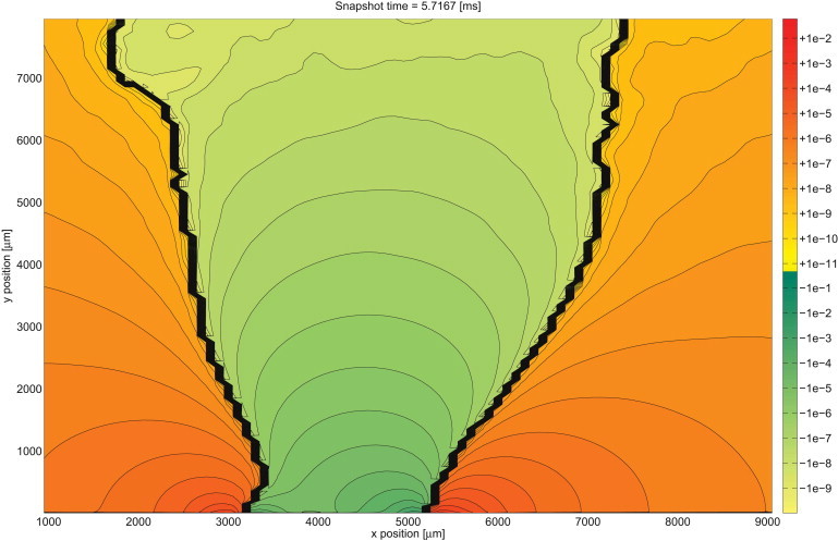
Snapshot of the whole extracellular potential. A contour plot of the logarithmically scaled extracellular potential at a fixed time point. The domain was cut at the left, right, and upper boundary to exclude artifacts introduced by the boundary where the potential is almost zero and switches signs due to small numerical errors.
The amplitudes of the potential are differing by several orders of magnitude among the intracellular values (∼100 mV), the extracellular values close to the membrane (up to a few 100 μV), and some millimeters away from the membrane (fractions of 1 μV).
The influence of potential and concentration changes on the local charge redistribution can be observed separately by studying the ion flux from Fig. S3 and Fig. S4, for each ion species. It gives a good impression about the complex interplay of drift and diffusion causing ion movement close to the membrane.
Comparison with line source approximation model
The line source approximation introduced in Holt and Koch (7) is widely used as an effective model to compute the extracellular potential at any point in space, using only the values of the membrane currents at a finite number of line segments,
| (13) |
where r is the radial distance from the line of length Δs, h is the longitudinal distance from the end of the line, and l = Δs + h is the distance from the start of the line. The parameter ρ describes the resistivity of the extracellular medium. This model is very convenient, especially when using cable equation models based on a line segment approximation of the original neuron geometry.
For the electrodiffusion model, the computed extracellular field can easily be compared with the LSA results, as the membrane currents are explicitly known from the internal membrane flux boundary conditions, so they can be inserted into the LSA expression from Eq. 13 directly. The resistivity ρ was chosen manually in such a way that the negative peaks N1 of electrodiffusion and LSA match for a fixed position close to the membrane (≈1 μm in this case). This resulted in a value of ρ = 37.4 Ωcm, corresponding to a conductivity of σ = 2.67 S/m, which is ∼30–50% higher than experimentally obtained values for cerebrospinal fluid (24,25). Fig. 9 shows the comparison of potential time courses for LSA and electrodiffusion (ED) models at various distances from the membrane. Additionally, the difference between the two curves is plotted.
Figure 9.
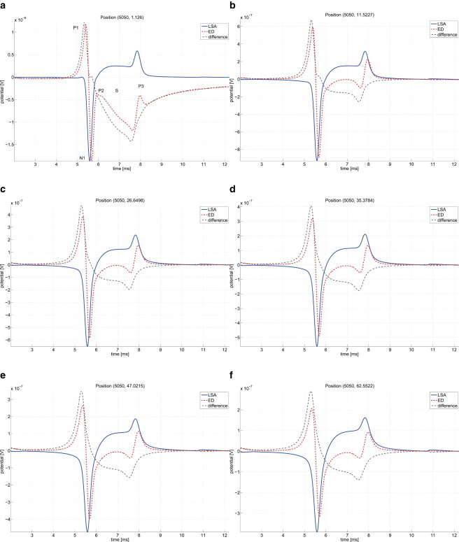
Comparison of electrodiffusion and line source approximation. The time courses of extracellular potentials calculated by electrodiffusion (ED, dashed line) and line source approximation (LSA, solid line) models are compared at different distances from the membrane (a–f) for a fixed x coordinate. The similar shape for the part between N1 and P3 is apparent, but the first peak P1 is missing in LSA. (Dash-dotted line) Difference between the two curves.
One can see that both signals show a set of common features: The negative peak N1 following the dominating sodium current in the beginning of an AP, followed by a transition phase of slower variation (S) and the less pronounced positive peak P3 during the repolarization phase. But the electrodiffusion signal shows another sharp positive peak (P1) right in the beginning, which is not present in the LSA model.
The difference between the LSA and ED curves resembles a distorted AP waveform that gets smeared out over distance. Our explanation for the difference is that the ED potential results from two contributors: The potential generated by membrane currents (as in LSA) and, in addition, an AP echo part directly coming from the intracellular potential wave traveling along the axon. The difference plotted in Fig. 9 would then largely represent the latter part of the signal stemming from the AP echo alone.
Looking closely, there is also a slight delay in the ED signal—i.e., the N1 peak is time-shifted by ∼90 μs to the LSA signal, with the same holding for the P3 peak. These differences cannot be a result of the membrane current sources, as these are identical for both models, so it has to be an effect of the extracellular medium. We attribute the delay to the local effects of redistributing ion concentrations, especially in the Debye layer with its large concentration gradients, leading to a delayed transduction of the electric field, wheras the LSA model assumes an instantaneous response to the membrane current sources.
Conclusions
In this article we presented results from the numerical simulation of an AP traveling along an active axonal membrane and its spread into the extracellular space. To our knowledge, this is the first time that such detailed information about the dynamics of ion concentrations and the electric potential in time and space were given on this scale. Recent applications of PNP theory to neurons have been done in Lopreore et al. (11) and Mori et al. (13). In contrast to these studies, we paid special attention in resolving the Debye layer explicitly, thereby accounting for the effects of large concentration gradients. This also adds the benefit that both steady-state concentrations and equilibrium-channel reversal potentials can be validated directly, using Poisson-Boltzmann and Nernst equations, respectively.
The evolution of the LFP signal and its various features have been analyzed particularly. We showed that the large concentration gradients have a significant impact on the near-field extracellular field. A detailed evaluation of the results shows the complex interplay of potential and concentration changes on the local ion redistribution. The intricate structure of the results (compare to Fig. 6) reveals that the neural membrane dynamics—even in this very simple case of a minimal set of only two channel types—is highly nontrivial and that a detailed study is indeed justified.
The main finding is that the electrodiffusion model shows significant deviations from the well-established line source approximation model, in particular a positive peak at the beginning of the LFP signal, directly caused by the intracellular potential propagating into extracellular space. This implies that there is a second component next to membrane currents contributing to the generation of the LFP signal, which we termed the “AP echo”. This component had a strong effect in our simplified model, but this might look differently in other situations, e.g., in myelinated fibers. In Gold et al. (5), the LSA showed a good agreement with experimental data, although the authors reported difficulties in fitting the intra- and extracellular data simultaneously. However, there is also experimental evidence that the LFP waveforms emerging from the electrodiffusion model occur in unmyelinated afferent nerve fibers (26) as well as in hippocampal CA1 neurons (27).
It remains to be shown in which situations the LSA model gives a valid approximation, and under which conditions the effect of the AP echo on the extracellular potential cannot be neglected. An experimental study using juxta- and extracellular recordings of axon fibers should be able to validate the reported LFP attenuation and change in signal shape from the Debye layer to near-field and the more distant extracellular regime.
We emphasize that our model could numerically be simulated with standard methods, i.e., with conforming finite elements for the spatial and an implicit Euler method for the time discretization. However, some essential precautions had to be taken to ensure a stable and efficient method, namely:
The grid had to resolve the Debye layer close to the membrane in the direction normal to the membrane. For the x direction, a much coarser mesh size was sufficient.
The PNP system had to be solved in a fully coupled fashion, as an operator-splitting approach dramatically reduced the time-step size needed for computing a nonoscillatory solution.
The system had to be carefully equilibrated before setting a stimulus, as the concentration profile toward the membrane had to reach steady state to get meaningful reversal potentials for each ion channel.
The choice of an implicit time-stepping scheme took advantage of higher stable time-step values and accounted for the diffusion-dominance in the Nernst-Planck equation that we observed for parameters in the physiological range.
The application of a threshold volume scaling was crucial to compensate the large differences of residual magnitudes introduced by the drastically varying cell volumes in this cylinder geometry. With this, the Newton iteration was able to converge even for large domain sizes—using the same error tolerances as for a plain two-dimensional simulation—with an only slightly lower average time-step size.
The model used here does not claim to be fully realistic nor complete from the biological point of view. Instead it should be considered as a first attempt to model the dynamics of neural systems on this spatial scale. Particularly, the idealized setup of a single axon fiber in an extracellular space consisting exclusively of fluid will rarely occur in reality. Additionally, no synaptic currents were regarded, which are thought to be the main contributors of electroencephalography and LFP signals (28,29). However, the characteristic features of the LFP signal could be explained by the interplay of ion channel currents and electrolyte dynamics alone in this model.
To arrive at more realistic models, the greatly simplified geometry from this model will have to be replaced in a later study by either explicitly incorporating a complex reconstructed extracellular geometry, or by finding effective material parameters (diffusivity of ions, electric permittivity) for representative intra- and extracellular media without explicitly modeling nearby cells.
For the axon geometry, assessing the impact of branching structures and ultimately, a complete attached single cell morphology with hundreds of compartments and synapses, is of great interest. Because these complicated geometries cannot be handled by a cylinder symmetry, a full three-dimensional simulation has to be carried out for this, necessitating the parallelization of our simulator.
Further model refinement concerning the detailed structure and properties of the active membrane (channel types and conductivities, surface charges, myelination) will have to be done when comparing the results with experimental data.
Acknowledgments
We thank Prof. Andreas Draguhn and Dr. Martin Both for fruitful discussions and information about extracellular signals in slice recordings. Many thanks also to Steffen Müthing for helping with the dune-multidomain setup and the anonymous reviewers for their valuable comments.
This work was funded through a grant from the German Ministry of Education and Research (BMBF No. 01GQ1003A).
Supporting Material
References
- 1.Hodgkin A.L., Huxley A.F. A quantitative description of membrane current and its application to conduction and excitation in nerve. J. Physiol. 1952;117:500–544. doi: 10.1113/jphysiol.1952.sp004764. [DOI] [PMC free article] [PubMed] [Google Scholar]
- 2.Rall W. Methods in Neuronal Modeling. MIT Press; Cambridge, MA: 1989. Cable theory for dendritic neurons; pp. 9–92. [Google Scholar]
- 3.Hines M.L., Carnevale N.T. The NEURON simulation environment. Neural Comput. 1997;9:1179–1209. doi: 10.1162/neco.1997.9.6.1179. [DOI] [PubMed] [Google Scholar]
- 4.Bower J., Beeman D., Wylde A. Telos Publishing; Candor, New York: 1995. The Book of GENESIS: Exploring Realistic Neural Models with the General Neural Simulation System. [Google Scholar]
- 5.Gold C., Henze D.A., Buzsáki G. On the origin of the extracellular action potential waveform: a modeling study. J. Neurophysiol. 2006;95:3113–3128. doi: 10.1152/jn.00979.2005. [DOI] [PubMed] [Google Scholar]
- 6.Bédard C., Kröger H., Destexhe A. Modeling extracellular field potentials and the frequency-filtering properties of extracellular space. Biophys. J. 2004;86:1829–1842. doi: 10.1016/S0006-3495(04)74250-2. [DOI] [PMC free article] [PubMed] [Google Scholar]
- 7.Holt G.R., Koch C. Electrical interactions via the extracellular potential near cell bodies. J. Comput. Neurosci. 1999;6:169–184. doi: 10.1023/a:1008832702585. [DOI] [PubMed] [Google Scholar]
- 8.Bédard C., Kröger H., Destexhe A. Model of low-pass filtering of local field potentials in brain tissue. Phys. Rev. E Stat. Nonlin. Soft Matter Phys. 2006;73:051911. doi: 10.1103/PhysRevE.73.051911. [DOI] [PubMed] [Google Scholar]
- 9.Bédard C., Destexhe A. Macroscopic models of local field potentials and the apparent 1/f noise in brain activity. Biophys. J. 2009;96:2589–2603. doi: 10.1016/j.bpj.2008.12.3951. [DOI] [PMC free article] [PubMed] [Google Scholar]
- 10.Pettersen K.H., Hagen E., Einevoll G.T. Estimation of population firing rates and current source densities from laminar electrode recordings. J. Comput. Neurosci. 2008;24:291–313. doi: 10.1007/s10827-007-0056-4. [DOI] [PubMed] [Google Scholar]
- 11.Lopreore C.L., Bartol T.M., Sejnowski T.J. Computational modeling of three-dimensional electrodiffusion in biological systems: application to the node of Ranvier. Biophys. J. 2008;95:2624–2635. doi: 10.1529/biophysj.108.132167. [DOI] [PMC free article] [PubMed] [Google Scholar]
- 12.Mori Y. From three-dimensional electrophysiology to the cable model: an asymptotic study. Arxiv preprint. 2009;arXiv 0901.3914. [Google Scholar]
- 13.Mori Y., Fishman G.I., Peskin C.S. Ephaptic conduction in a cardiac strand model with 3D electrodiffusion. Proc. Natl. Acad. Sci. USA. 2008;105:6463–6468. doi: 10.1073/pnas.0801089105. [DOI] [PMC free article] [PubMed] [Google Scholar]
- 14.Xylouris K., Queisser G., Wittum G. A three-dimensional mathematical model of active signal processing in axons. Comput. Visualization Sci. 2010;13:409–418. [Google Scholar]
- 15.Lu B., Holst M.J., Zhou Y.C. Poisson-Nernst-Planck equations for simulating biomolecular diffusion-reaction processes. I. Finite element solutions. J. Comput. Phys. 2010;229:6979–6994. doi: 10.1016/j.jcp.2010.05.035. [DOI] [PMC free article] [PubMed] [Google Scholar]
- 16.Koch C. Oxford University Press; Oxford, UK: 2004. Biophysics of Computation: Information Processing in Single Neurons. [Google Scholar]
- 17.Demmel J.W., Eisenstat S.C., Liu J.W.H. A supernodal approach to sparse partial pivoting. SIAM J. Matrix Anal. Appl. 1999;20:720–755. [Google Scholar]
- 18.Bastian P., Blatt M., Sander O. A generic grid interface for parallel and adaptive scientific computing. I. Abstract framework. Computing. 2008;82:103–119. [Google Scholar]
- 19.Bastian P., Blatt M., Sander O. A generic grid interface for parallel and adaptive scientific computing. II. Implementation and tests in DUNE. Computing. 2008;82:121–138. [Google Scholar]
- 20.Bastian P., Heimann F., Marnach S. Generic implementation of finite element methods in the distributed and unified numerics environment (DUNE) Kybernetika. 2010;46:294–315. [Google Scholar]
- 21.Müthing S., Bastian P. Dune-multidomaingrid: a metagrid approach to subdomain modeling. In: Dedner A., Flemisch B., Klöfkorn R., editors. Advances in DUNE. Springer; Berlin, Germany: 2012. pp. 59–73. [Google Scholar]
- 22.Müthing, S. 2012. Dune-multidomain. Accessed December 4, 2012. http://users.dune-project.org/projects/dune-multidomain.
- 23.Schönke J. Unsteady analytical solutions to the Poisson-Nernst-Planck equations. J. Phys. A. 2012;45:455204. [Google Scholar]
- 24.Baumann S.B., Wozny D.R., Meno F.M. The electrical conductivity of human cerebrospinal fluid at body temperature. IEEE Trans. Biomed. Eng. 1997;44:220–223. doi: 10.1109/10.554770. [DOI] [PubMed] [Google Scholar]
- 25.Gabriel S., Lau R.W., Gabriel C. The dielectric properties of biological tissues: III. Parametric models for the dielectric spectrum of tissues. Phys. Med. Biol. 1996;41:2271–2293. doi: 10.1088/0031-9155/41/11/003. [DOI] [PubMed] [Google Scholar]
- 26.Weidner C., Schmidt R., Torebjörk H.E. Time course of post-excitatory effects separates afferent human C fiber classes. J. Physiol. 2000;527:185–191. doi: 10.1111/j.1469-7793.2000.00185.x. [DOI] [PMC free article] [PubMed] [Google Scholar]
- 27.Csicsvari J., Hirase H., Buzsáki G. Oscillatory coupling of hippocampal pyramidal cells and interneurons in the behaving Rat. J. Neurosci. 1999;19:274–287. doi: 10.1523/JNEUROSCI.19-01-00274.1999. [DOI] [PMC free article] [PubMed] [Google Scholar]
- 28.Buzsáki G., Anastassiou C.A., Koch C. The origin of extracellular fields and currents—EEG, ECoG, LFP and spikes. Nat. Rev. Neurosci. 2012;13:407–420. doi: 10.1038/nrn3241. [DOI] [PMC free article] [PubMed] [Google Scholar]
- 29.Nunez P., Srinivasan R. Oxford University Press; Oxford, UK: 2005. Electric Fields of the Brain: the Neurophysics of EEG. [Google Scholar]
- 30.Carnevale, N. 2012. Vtrap derived. Accessed December 4, 2012. http://www.neuron.yale.edu/phpBB/viewtopic.php?f=15&t=1075.
Associated Data
This section collects any data citations, data availability statements, or supplementary materials included in this article.