Aged particles derived from emissions of coal-fired power plants: The TERESA field results

Abstract

The Toxicological Evaluation of Realistic Emissions Source Aerosols (TERESA) study was carried out at three US coal-fired power plants to investigate the potential toxicological effects of primary and photochemically aged (secondary) particles using in situ stack emissions. The exposure system designed successfully simulated chemical reactions that power plant emissions undergo in a plume during transport from the stack to receptor areas (e.g., urban areas). Test atmospheres developed for toxicological experiments included scenarios to simulate a sequence of atmospheric reactions that can occur in a plume: (1) primary emissions only; (2) H₂SO₄ aerosol from oxidation of SO₂; (3) H₂SO₄ aerosol neutralized by gas-phase NH₃; (4) neutralized H₂SO₄ with secondary organic aerosol (SOA) formed by the reaction of α-pinene with O₃; and (5) three control scenarios excluding primary particles. The aged particle mass concentrations varied significantly from 43.8 to 257.1 μg/m³ with respect to scenario and power plant. The highest was found when oxidized aerosols were neutralized by gas-phase NH₃ with added SOA. The mass concentration depended primarily on the ratio of SO₂ to NO_x (particularly NO) emissions, which was determined mainly by coal composition and emissions controls. Particulate sulfate (H₂SO₄ + neutralized sulfate) and organic carbon (OC) were major components of the aged particles with added SOA, whereas trace elements were present at very low concentrations. Physical and chemical properties of aged particles appear to be influenced by coal type, emissions controls and the particular atmospheric scenarios employed.

Introduction

Epidemiological studies have reported significant associations between increases in the levels of particulate pollutants (PM_2.5: particles with diameter below 2.5 μm; PM₁₀: particles with diameter below 10 μm) and excess daily morbidity and mortality from respiratory and cardiovascular causes (Pope et al., 1992; Dockery et al., 1993; Schwartz and Moris, 1995). The associations have been observed even when the concentrations are below the US National Ambient Air Quality Standards (NAAQS). Toxicological studies using urban concentrated ambient particles (CAPs) have shown pulmonary, cardiac, or systemic effects of short-term particle exposure in rats or dogs (Clarke et al., 2000; Batalha et al., 2002; Gurgueira et al., 2002; Wellenius et al., 2003, 2004).

Coal-fired power plants are used to generate a significant amount of the electricity consumed in the United States (AER, 2006). They also contribute significantly to ambient fine particles regionally, especially in the eastern United States, from the photochemical oxidation of SO₂ to sulfate during transport. Several source apportionment studies have reported that coal-fired power plants are significant contributors to sulfate, and as a result, fine particle mass in urban atmospheres (Watson et al., 2002; Chow et al., 2004). Fly ash formed from coal combustion is primarily removed by emissions control devices (typically electrostatic precipitators) at coal-fired power plants and therefore only a small fraction of the ash is emitted to the atmosphere (Sandelin and Backman, 2001).

Given the significant contribution of power plants to PM_2.5, there is great interest in investigating the toxicity of particles derived from coal-fired power plants. Numerous studies have reported on adverse health effects in laboratory rodents of coal fly ash (CFA) exposure (Raabe et al., 1982; Chen et al., 1990; Dormans et al., 1999; Gilmour et al., 2004; Smith et al., 2006). These studies have been conducted in a laboratory setting using either pilot-scale coal combustors or CFA collected from coal-fired power plants. However, because these studies only involved primary particles, their relevance to human exposure is unclear given the small amounts of primary particles in the atmosphere, and these studies were unable to evaluate the toxicity of secondary particles derived from coalfired power plants. Atmospheric aging alters the composition of emissions and therefore may modify toxicity. In particular, the formation of secondary organic aerosol from volatile organic compounds (VOCs) may produce reactive species with the potential to induce health effects (Venkatachari and Hopke, 2008; Chen and Hopke, 2009; Rohr et al., 2003). More recently, a laboratory-based program was carried out to develop a Simulated Downwind Coal Combustion Atmosphere (SDCCA) that was subsequently employed in toxicological experiments. Like the one described herein, this atmosphere was intended to consider both the primary and secondary particulate components derived from coal combustion (McDonald et al., 2010).

The Toxicological Evaluation of Realistic Emission Source Aerosols (TERESA) study investigated the toxicity of primary and simulated aged particles derived from coal combustion. This study was designed to address limitations in previous studies of CFA exposure. The study involved on-site sampling, dilution, and aging of coal combustion emissions at three pulverized coal-fired power plants across the United States, followed by animal exposures incorporating a number of toxicological endpoints. This paper describes the on-site sampling, dilution, and aging process as well as the physical and chemical properties of aged particles from the power plants. The toxicological effects of simulated aged particles are discussed in the related series of TERESA papers (Godleski et al., 2011a, 2011b; Diaz et al., 2011; Lemos et al., 2011; Wellenius et al., 2011).

Experimental methods

Coal-fired power plants

In order to optimize potential variability in exposure, three coal-fired power plants using different coal types and different emissions control devices were selected for the TERESA study. Detailed characteristics of the power plants are described elsewhere (Godleski et al., 2011a). Briefly, all tests were conducted at a single unit at each of the three power plant sites. The first power plant (“Plant 1,” located in the Upper Midwest) burned a low sulfur (~0.2% S) subbituminous coal from the Wyoming Powder River Basin. Plant 1 is comprised of two 600-MW units, each equipped with a Riley Stoker turbo-fired boiler, and used an electrostatic precipitator (ESP) for particle emission control. The second plant (“Plant 2,” located in the Southeast) used a tangentially fired boiler to burn low-medium sulfur (~1.0% S) bituminous coals from various regions, including Kentucky, West Virginia, and South America. The utility consisted of a single unit with an electric power capacity of 650 MW. It used an ESP for particle emission control and employed selective catalytic reduction (SCR) for NO_x (NO + NO₂) emission control. The third plant (“Plant 3,” located in Midwest) used a wall-fired boiler to burn a high sulfur (~3.0% S) bituminous coal from Indiana and was comprised of two units with an electric power capacity of 500 MW each. In contrast to the first two plants, each unit at Plant 3 had a wet flue gas desulfurization (FGD) scrubber with an inhibited oxidation process to reduce SO₂ emission, along with an ESP and an SCR. The wet FGD scrubber used limestone as alkaline slurry to absorb SO₂ from the flue gas and produce calcium-sulfur compounds. We believe that it is likely that only very small amounts of limestone derived from the wet FGD scrubber at Plant 3 contributed to the particles measured in the exposure atmospheres, because (1) the limestone was mechanically ground to powder; (2) this process produces very small amounts of submicron particles; and (3) our sampling apparatus collected primarily submicron particles.

Continuous stack sampling and dilution

For the TERESA study, field sampling was conducted for 7 months (April–November, 2004) at Plant 1, 7 months (February–September, 2005) at Plant 2, and 3 months (June– September, 2006) at Plant 3. This included on-site sampling, dilution, and aging of coal combustion emissions conducted using a mobile reaction laboratory (the front bus) and animal exposure using a mobile toxicology laboratory (the back trailer), as shown in Figure 1. Figure 2 is a schematic diagram showing the path from the diluted stack emissions to the exposure atmosphere, with additional dilutions at different locations in this path, and sampling ports.

Figure 1.

Mobile laboratory. (See colour version of this figure online at www.informahealthcare.com/iht)

Figure 2.

Overview of the dilution and sampling scheme: Total dilution factors were approximately 1700, 2000, and 1000 at Plants 1 though 3, respectively. (See colour version of this figure online at www.informahealthcare.com/iht)

Stack emissions were extracted at a port on the duct passing into the stack downstream of the emissions control devices, and then diluted with compressed dry, filtered air with a dilution factor of 75–150 using a stack extraction system designed for the study, as shown in Figure 3a and b. The dilution factors were sufficient to avoid water condensation when the stack emissions were cooled from stack temperature to ambient temperature, and to attain SO₂ and NO_x (NO + NO₂) concentrations that were suitable for our experiments. Only a small amount of the diluted stack emissions were used for experiments and the rest was vented out of the sample flow. A relatively high flow of diluted emissions in the transmission tube kept the residence time short enough to minimize potential particle losses and artifact formation during transport from the stack to the reaction laboratory.

Figure 3.

Schematic diagram of the stack extraction systems: (a) Plants 1 and 2; (b) Plant 3.

Continuous and stable sampling of stack emissions was required for the TERESA approach. An adequate flow with positive pressure of sufficiently diluted stack emissions was necessary to operate the chemical reaction chambers, which simulated pollutant transformations in the atmosphere. The stack extraction system used a stainless steel aspirator (Model JD-300; Vaccon, Medway, MA) to create the vacuum needed to continuously extract stack gas at a constant flow. The aspirator used 150–200 L/min of compressed dry, filtered air to create the vacuum, dilute the stack emissions, and then transport the diluted emissions under positive pressure through the transmission tubing to the mobile reaction laboratory. At Plants 1 and 2, the stack sampling flow was controlled using a stainless-steel restriction tube placed inside the stack (Figure 3a). Consequently, the dilution factor was about 130 at Plant 1 and about 150 at Plant 2.

Plant 3 used a wet FGD scrubber to reduce SO₂ emissions, along with an ESP and a SCR unit. Because the wet scrubber resulted in highly humid stack emissions, the extraction system used at the other two plants had to be modified to prevent water condensation. The new extraction probe (Figure 3b) consisted of concentric sampling tubes: an outer tube (183 cm long and 7.63 cm internal diameter [ID]) with a flow of dry, hot (about 100°C) filtered air for initial dilution of the wet stack emissions, and a thin inner tube (244 cm long and 1.27 cm ID) used to pass the initially diluted stack emissions into the aspirator. The inner tube was heated using an electric heating coil to prevent potential clogging due to water condensation. The stack sampling rate could be adjusted by changing the flow rate of hot, dry filtered air and by changing the amount of vacuum by controlling the total flow of dry filtered air into the aspirator. As a result, the dilution factor of 75 was used at Plant 3.

Photochemical aging and atmospheric scenarios

The reaction laboratory contained two reaction chambers. The first reaction chamber was used to produce H₂SO₄ aerosol from the oxidation of SO₂, whereas the second reaction chamber was used to neutralize H₂SO₄ aerosol and/or to form secondary organic aerosol (SOA).

The SOA was derived from the reaction of α-pinene with O₃ in the chamber. We chose α-pinene as a VOC precursor because it is known as the most important terpene emitted on a global scale (Kanakidou et al., 2005).

Stack emissions diluted initially on the stack (“Diluted stack emissions”) were transported to the first chamber through a 25–30 m stainless steel tube (2.54 cm outer diameter [OD], 2.16 cm ID). In addition, one nonselective countercurrent parallel plate membrane diffusion denuder (“parallel plate diffusion denuder,” with 85–90% gas removal efficiency) was used to remove excess gaseous co-pollutants during transfer from the first chamber to the second chamber, and a second denuder was used downstream of the second chamber (Ruiz et al., 2006). Detailed descriptions of the photochemical chambers are available elsewhere (Ruiz et al., 2007a, 2007b; Godleski et al., 2011a).

In order to simulate atmospheric transformations that coal power plant emissions undergo in a plume, the following scenarios were chosen: (1) primary emissions only (“P”); (2) the oxidation of SO₂ to form H₂SO₄ aerosol, along with primary particles (“PO”); (3) the oxidation of SO₂ plus the reaction of α-pinene with ozone to form SOA, along with primary particles (“POS”); (4) the neutralization of H₂SO₄ aerosol by NH₃, along with primary particles and SOA (“PONS”); (5) a control scenario including oxidation of SO₂ scenario that included primary gases but excluded primary particles (“O”); (6) the O control scenario with added SOA (“OS”); and (7) a control scenario with no primary particles or gases and only SOA produced using particle-free ambient air (“S”). The control scenarios (“O,” “OS,” and “S”) were conducted only at Plant 3.

Sampling and analytical methods

Sampling ports were installed upstream/downstream of the first chamber (Ports A and B, respectively), downstream of the second chamber, and upstream of the animal exposure chamber in the toxicology laboratory (Port C), as shown in Figure 2. Primary emissions, aged particles, and gases were measured at these ports during and following the aging process. In the toxicology laboratory, there were five individual chambers in parallel drawing 1.5 L/min each for rat exposures, along with a manifold with ports for characterization of exposure atmospheres. This paper presents the following results: (1) physical and chemical properties of the particles and gases used for animal exposures measured at the port (Port C) in the toxicology laboratory; (2) primary particle mass, size distribution, and elemental composition measured at the upstream port (Port A) of the first chamber (diluted stack emissions); and (3) the sulfate concentration measured at the upstream and downstream ports (Ports A and B, respectively) of the first chamber to determine the SO₂ conversion ratio.

A tapered element oscillating microbalance (TEOM) (Model 1400a; Rupprecht & Patashnick, Waltham, MA) was used to continuously monitor particle mass concentrations during animal exposure at the first two plants. The TEOM was run at above-ambient temperature (50°C) during sampling to minimize the effect of water collected on the filter. Particle size distributions for primary and aged particles were measured using a scanning mobility particle sizer (SMPS) (Model 3934; TSI, Shoreview, MN) and an aerodynamic particle sizer (APS) (Model 3321; TSI). Because both the TEOM and the particle sizers were inoperable after use at the first two plants (due to extensive exposure to strong acidic conditions), a DustTrak (Model 8520; TSI) aerosol monitor replaced the other instruments at Plant 3 to continuously monitor particle mass concentrations; consequently, particle size distributions were not measured at this plant.

At all three power plants, particle number concentration was monitored using a portable condensation particle counter (CPC) (Model 3022a; TSI). Continuous gaseous co-pollutants were measured, including (1) NO and NO₂ (chemiluminescence; Model 49C; Thermo Environmental Instruments, Waltham, MA); (2) SO₂ (pulsed fluorescence; Model 43C; Thermo Environmental Instruments); and (3) O₃ (ultraviolet [UV] photometry; Model 42C; Thermo Environmental Instruments), for diluted stack emissions and exposure atmospheres. Temperature and relative humidity were measured using a Hygrometer sensor (Model 411; Omega Engineering, Stamford, CT).

In addition, the following integrated measurements were carried out to characterize exposure atmospheres: Teflon-membrane filters were used to measure gravimetric mass, trace elements by X-ray fluorescence (XRF), specific components of SOA by gas chromatography–mass spectrometry (GC-MS), and water-soluble ions by ion chromatography (IC). A prefired quartz filter was used to measure organic (OC) and elemental carbon (EC) by thermal optical reflectance (TOR) analytical method. Gravimetric mass concentrations were obtained from postweight measurements following equilibration at 40% relative humidity (RH) and 22°C. A 2,4-dinitrophenylhydrazine (DNPH) cartridge was used to quantify formaldehyde, acetaldehyde, and acetone by high-performance liquid chromatography (HPLC). A Tenax tube was used to measure α-pinene by GC-MS. Following 6-h chamber stabilization (except for the P and S scenarios), integrated samples were collected during the 6-h exposure period on each exposure day, except for 5-h samples during the 5-h mycocardial infarction (MI) rat model exposures (Wellenius et al., 2011).

Results and discussion

Diluted stack emissions

Stack emissions were diluted initially by a factor of 75–150 in the stack extraction system on the duct. Particle size distribution (discussed below), particle mass concentration, and concentrations of gaseous species were monitored at Port A, prior to the first reaction chamber to characterize the diluted stack emissions. Concentrations of gases and primary particles entering the first reaction chamber are summarized in Table 1.

Table 1.

Diluted stack emissions in the stack extraction system.

	SO2(ppb)	NO (ppb)	NO2(ppb)	SO2/NOx ratio	Primary particles (μg/m3)
Plant 1a
P (n = 4)b	2009 (692–2621)c	1875 (379–2197)	25 (2–232)	1.1	17 (5–30)
PO (n = 1)	838 (351–1188)	657 (406–836)	4 (2–29)	1.1	2
POS (n = 4)	2860 (2733–3080)	2279 (2014–2478)	34 (6–82)	1.3	5 (3–6)
PONS (n = 10)	1979 (1001–3298)	1681 (998–3301)	36 (3–186)	1.2	3 (2–6)
Plant 2a
P (n = 4)	4373 (3603–5264)	169 (129–203)	8 (2–25)	22.0	1 (0–1)
PO (n = 4)	3369 (2292–6360)	104 (74–154)	12 (4–27)	34.0	9 (0–31)
POS (all, n = 12)	3942 (2386–5756)	257 (60–521)	9 (1–32)	13.0	6(0–28)
POS (non-SCR, n = 4)	4659 (3640–5416)	470 (401–521)	8 (1–19)	9.4	2 (1–3)
POS (SCR, n = 8)	3534 (2386–5756)	136 (60–304)	10 (4–27)	35.0	8 (0–28)
PONS (n = 4)	4547 (2819–6123)	165 (99–302)	14 (8–32)	22.5	2 (0–3)
Plant 3a
P (n = 4)	1824 (747–6407)	760 (275–1602)	11 (1–51)	2.3	968 (520–1417)
PO (n = 4)	1335 (792–1873)	591 (330–1025)	10 (2–45)	2.2	173 (98–255)
POS (n = 8)	1418 (485–3937)	434 (128–1603)	11 (2–75)	3.5	790 (527–1116)
PONS (n = 4)	1277 (613–2586)	335 (148–800)	18 (2–63)	4.3	467(344–708)
OS (n = 4)	1027 (142–5074)	368 (116–1602)	10 (2–46)	2.5	—d
O (n = 4)	1092 (439–1824)	398 (148–615)	11 (1–60)	2.8	—
S (n = 4)	55 (19–160)	2 (2–16)	7 (3–27)	22.2	—

^aInitial dilution factors on the stack: about 130 times at Plant 1, about 150 times at Plant 2, and about 75 times at Plant 3.

^bNumber of primary particle samples measured at Part A. For SO₂ and NOx, continuous measurements were used for data summary.

^cAll values are an average and range.

^dPrimary particles for OS and O scenarios were zero because a HEPA filter was used to remove primary particles upstream of the first reaction chamber.

Gaseous species

For all species and for all three plants, there was a fair amount of day-to-day variation in primary emissions, both within and between exposure days. This variation was most likely due to the inherent variation in power plant operations because a relatively constant factor was used to dilute stack emissions at each plant during the respective study periods. The concentrations of gaseous species are likely to depend on coal type and the emissions controls employed at each coal-fired power plant.

At Plant 1, equipped with an ESP, a higher NO concentration was observed in diluted stack emissions compared to the other plants with an SCR unit for NO_x (NO + NO₂) emission control. This led to a lower ratio of SO₂ to NO_x concentrations, which is expected to decrease the formation rate of secondary sulfate particles. At Plant 2, a higher ratio of SO₂ to NO was found in diluted stack emissions compared to the other plants because the plant used low-to-medium sulfur (~1.0% S) bituminous coal with an SCR. Note that the SCR unit was operational at Plant 2 during “ozone season” (May–September, 2005). The results for the POS scenario thus can be compared for the SCR-off period in March (the first 4 days) and for the SCR-on period during the period of May to September (the last 8 days). NO emissions during the SCR-on period were about 25% of those during the SCR-off period.

Diluted stack emissions at Plant 3 used a higher sulfur bituminous coal had a lower SO₂ concentration (due to the use of a wet FGD scrubber), as compared to the other plants. Lower SO₂ stack emission required less stack dilution to produce comparable sulfate in the first reaction chamber. In contrast, highly water content of stack emissions produced by the scrubber required a higher dilution to prevent water condensation in the transmission tube. A new stack extraction probe (Figure 3b) was designed to solve this dilemma, which made it possible to run at a lower initial dilution. A validation test of the new stack extraction system was carried out during a period of relatively constant particle emissions at Plant 3. Primary particle mass concentration was measured downstream of the extraction system with different dilution factors. Dilution factors used were between about 20 and 70. Sampling time varied from 2 to 15 h at a sampling flow of 10 L/min. During the test, diluted primary particle mass concentration ranged from 104 to 2544 μg/m³, with an average of 1468 μg/m³. A consistent relationship (slope = −47, R² = .98) was found between primary particle mass concentrations and dilution factors. This strong correlation indicates that the new extraction system prevented the clogging due to water condensation in the sampling probe that had been observed for this plant when using the original extraction system.

At Plant 3, diluted stack emissions had a large variability. For example, SO₂ concentration diluted at a factor of 75 varied from 142 to 5074 ppb during the period of the OS scenario. The most likely explanation for this instability was the occasionally unstable operation of the scrubber; two or three times during the entire study period, the scrubber was shut down. However, the shutdowns did not occur during animal exposures. The instability may also have been influenced by varying sulfur content in the coal.

Primary particles

As shown in Table 1, much lower concentrations of primary particles were observed at Plant 1 (an average of 6.2 μg/m³, n = 19) and Plant 2 (an average of 4.7 μg/m³, n =24) compared to Plant 3 (an average of 637.8 μg/m³, n = 20). When the concentrations were determined for direct emissions (downstream of the ESP at Plants 1 and 2, and downstream of FGD scrubber at Plant 3), taking into account dilution in the extraction system, the mean direct emissions of primary particles were 0.8 mg/m³ at Plant 1, 0.7 mg/m³ at Plant 2, and 47.8 mg/m³ at Plant 3. The difference in primary particle emissions likely results mainly from different emissions control configurations, rather than different coal types (see discussion below).

SO₂ conversion ratio

Diluted SO₂ was converted to H₂SO₄ in the first chamber, under conditions of UV irradiation and the addition of O₃ and water vapor. The SO₂ conversion ratio was affected by the ratio of SO₂ to NO_x concentrations, when keeping the other parameters constant (total added ozone, humidity, and intensity of UV irradiation). This is because the SO₂ to H₂SO₄ conversion is restricted in the presence of NO_x. The NO_x-OH reaction competes with, and is faster than the SO₂-OH reaction (Luria et al., 1983; Seinfeld and Pandis, 1986). Consequently, with lower NO_x concentration there is greater excess of ozone (as a source of OH radical, under sufficient UV irradiation and water vapor), which resulted in a higher reaction rate of SO₂. The SO₂ conversion ratio was calculated as follows:

$${\text{SO}}_2\text{conversion}\text{ratio}=(F_{\text{sulfate}}-P_{\text{sulfate}})/P_{{\text{SO}}_2}$$

Where, F_sulfate is the sulfate concentration (μg/m³) downstream of the chamber; P_SO2 is the SO₂ concentration (μg/m³ sulfate equivalent) transmitted into the chamber; and P_sulfate is primary sulfate concentration (μg/m³) emitted from the stack. On average, the SO₂ conversion ratio was 16.7% at Plant 1 (Ruiz et al., 2007b). At Plant 2, a higher ratio of SO₂ to NO was found in diluted stack emissions compared to the other plants because the plant used higher sulfur coals with an SCR. The lower NO concentration resulted in a higher excess of ozone (for a fixed amount of ozone added), which made it possible to obtain a higher conversion ratio. For instance, NO emissions during the SCR-off period were 4 times higher than during the SCR-on period. On average, the SO₂ conversion ratio was 7.7% during the SCR-off period, whereas the ratio was 19.0% during the SCR-on period.

Diluted stack emissions at Plant 3 had relatively lower SO₂ and higher NO concentrations than those at Plant 2. Because sulfate was found to be a major component of primary particles, the primary sulfate concentration was deducted from the measured sum (F_sulfate) of primary plus secondary sulfate to calculate the SO₂ conversion ratio. On average, a higher conversion ratio (22.2%) was observed at Plant 3, which was most likely due to lower SO₂ concentrations entering the first chamber as compared to Plant 2.

Exposure atmospheres

Diluted stack emissions were additionally diluted about 12 times to be used for animal exposures. As a result, total dilution factors were approximately 1700, 2000, and 1000 at Plants 1, 2, and 3, respectively. Gaseous co-pollutants and particulate species measured at the sampling port (Port C) in the toxicological laboratory were characterized for all exposure atmospheres. Gaseous co-pollutants, temperature, and relative humidity are summarized for each scenario in Tables 2–4, for each power plant, respectively. Particle mass and its constituents are also summarized by scenario in Tables 5–7. Note that Plant 3 had two differences in the methods compared to the previous plants: (1) control scenarios (OS, O, and S) excluding primary particles were tested to evaluate the effects of primary particles and of atmospheric constituents; (2) because the TEOM, SMPS, and APS were not operational (as mentioned above), DustTrak Aerosol Monitors were used to measure continuous particle mass concentration.

Table 2.

Gaseous species concentrations and metrological parameters for each scenario at Plant 1.^a

Species	P (n = 4)b	PO(n = 3)	POS (n = 4)	PONS (n = 12)
O3(ppb)	1.0 ± 1.2c	26.9 ± 1.0	26.8 ± 6.9	26.6 ± 9.3
NO (ppb)	5.9 ± 3.7	3.9 ± 0.5	3.5 ± 2.9	3.7 ± 1.6
NO2(ppb)	6.7 ± 1.7	8.4 ± 1.8	17.5 ± 6.6	16.9 ± 7.0
(ppb)	NMd	31.7 ± 4.3	38.9 ± 8.3	34.5 ± 5.9
SO2(ppb)	0.7 ± 0.4	0.6 ± 0.1	1.6 ± 0.3	2.4 ± 0.5
HNO3
HONO (ppb)	2.7 ± 2.4	5.0 ± 1.0	11.2 ± 5.1	8.3 ± 2.5
NH3(ppb)	26.0 ± 26.5	9.9 ± 6.2	20.8 ± 3.8	5.9 ± 8.3
Formaldehyde (ppb)	NM	NM	13.4 ± 3.0	17.6 ± 4.3
Acetaldehyde (ppb)	NM	NM	2.9 ± 0.6	3.0 ± 0.7
Acetone (ppb)	NM	NM	6.7 ± 2.2	8.8 ± 5.2
α-Pinene (ppb)	NM	NM	0.1 ± 0.0	0.2 ± 0.1
Temp. (°C)	23.4 ± 0.5	23.9 ± 0.1	24.4 ± 0.4	24.4 ± 1.1
RH (%)	38.7 ± 7.6	18.4 ± 1.9	21.6 ± 5.5	37.7 ± 10.8

^aVOCs were not measured for the non-SOA scenarios, P and PO, but the concentrations were expected to have been close to typical ambient levels, resulting from relatively high dilution with particle-free ambient air, required to supply the exposure atmospheres and characterization measurements. ^bNumber of days.

^cAverage ± standard deviation.

^dNot measured.

Table 4.

Gaseous species concentrations and metrological parameters for each scenario at Plant 3.^a

Species	P(n = 4)b	PO(n = 4)	POS(n = 8)	PONS(n = 4)	OS(n = 4)	O(n = 4)	S(n = 4)
O3(ppb)	8.9 ± 3.3c	28.8 ± 8.8	29.2 ± 10.0	15.2 ± 6.6	19.9 ± 3.3	18.3 ± 4.2	21.0 ± 2.4
NO (ppb)	7.5 ± 2.4	9.4 ± 2.2	7.2 ± 1.5	6.3 ± 0.3	7.5 ± 3.8	5.8 ± 0.1	8.4 ± 0.7
NO2(ppb)	4.4 ± 0.8	3.7 ± 0.7	4.7 ± 1.2	3.7 ± 2.2	2.0 ± 0.4	2.5 ± 0.7	3.8 ± 1.0
SO2(ppb)	38.9 ± 15.7	34.7 ± 7.1	72.8 ± 83.2	23.1 ± 6.9	15.1 ± 6.6	24.4 ± 14.5	22.1 ± 8.1
HNO3(ppb)	0.0 ± 0.0	0.0 ± 0.1	0.1 ± 0.2	0.8 ± 1.0	0.3 ± 0.4	0.0 ± 0.0	0.1 ± 0.1
HONO (ppb)	3.5 ± 0.5	0.3 ± 0.6	2.9 ± 1.4	3.8 ± 3.1	1.2 ± 1.8	0.2 ± 0.4	1.0 ± 1.0
NH3(ppb)	0.3 ± 0.4	2.2 ± 4.3	2.3 ± 3.2	4.6 ± 4.4	8.3 ± 9.9	0.3 ± 0.6	3.3 ± 2.6
α-Pinene (ppb)	NMd	NM	0.4 ± 0.6	5.2 ± 5.6	2.3 ± 1.0	NM	3.0 ± 0.5
Temp. (°C)	23.3 ± 1.0	23.4 ± 1.2	23.8 ± 1.1	21.9 ± 0.3	24.5 ± 1.5	23.5 ± 0.0	23.9 ± 0.3
RH (%)	56.1 ± 17.6	26.5 ± 11.6	53.3 ± 19.6	53.0 ± 17.1	47.5 ± 10.2	38.7 ± 10.3	36.0 ± 2.0

^aAldehydes and acetone were not measured for this power plant because these concentrations were expected to be similar to the other two plants.

^bNumber of days.

^cAverage ± standard deviation.

^dNot measured.

Table 5.

Particle component concentrations at Plant 1.

Species	P(n = 4)a	PO(n = 3)	POS(n = 4)	PONS(n = 12)
Particle mass (μg/m3)b	1.0 ± 0.9c	46.0 ± 12.6	123.3 ± 28.4	154.9 ± 41.7
Gravimetric mass (μg/m3)	2.3 ± 2.6	69.5 ± 10.4	192.6 ± 73.3	212.6 ± 59.7
Continuous mass (μg/m3)d	0.0 ± 3.3	58.2 ± 5.8	138.2 ± 53.4	173.6 ± 56.8
Number (particles/cm3)	1726 ± 1277	6723 ± 3550	16,924 ± 4494	52,109 ± 11,951
Total sulfate (μg/m3)	0.2 ± 0.3	36.1 ± 7.7	55.8 ± 22.8	68.2 ± 28.8
Acidic sulfate (μg/m3)e	2.3 ± 0.4	27.6 ± 9.5	50.2 ± 21.6	14.7 ± 13.6
Neutralized sulfate (μg/m3)f	0.0 ± 0.0	8.4 ± 2.6	5.6 ± 3.4	53.6 ± 16.8
Nitrate (μg/m3)	0.1 ± 0.2	0.7 ± 1.2	0.3 ± 0.4	30.4 ± 8.2
Ammonium (μg/m3)	0.0 ± 0.0	3.2 ± 1.5	2.5 ± 1.1	20.7 ± 6.0
OC (μg/m3)	0.0 ± 0.0	2.6 ± 4.5	51.6 ± 3.4	53.6 ± 16.8
EC (μg/m3)	0.7 ± 0.8	3.1 ± 1.7	11.9 ± 9.1	5.0 ± 2.9
Na (ng/m3)	0.0 ± 0.0	0.0 ± 0.0	0.0 ± 0.0	0.0 ± 0.0
Mg (ng/m3)	0.2 ± 0.4	0.0 ± 0.0	2.2 ± 2.7	1.3 ± 2.7
Al (ng/m3)	2.2 ± 1.6	9.2 ± 6.6	13.9 ± 5.9	4.1 ± 5.3
Si (ng/m3)	1.9 ± 1.3	20.2 ± 16.3	10.9 ± 7.9	4.2 ± 4.9
P (ng/m3)	0.5 ± 0.4	2.3 ± 3.9	2.7 ± 1.8	0.6 ± 0.9
S (μg/m3)	0.1 ± 0.1	12.0 ± 2.6	18.6 ± 7.6	22.7 ± 9.6
K (ng/m3)	0.2 ± 0.2	0.0 ± 0.1	0.2 ± 0.2	0.3 ± 0.2
Ca (ng/m3)	7.0 ± 1.7	12.4 ± 7.5	49.8 ± 22.2	16.2 ± 17.4
Ti (ng/m3)	0.2 ± 0.3	0.5 ± 0.6	2.1 ± 1.1	0.7 ± 0.8
Cr (ng/m3)	3.0 ± 1.1	14.3 ± 24.8	0.0 ± 0.1	0.0 ± 0.0
Fe (ng/m3)	8.4 ± 4.2	60.0 ± 101.2	7.4 ± 4.2	2.8 ± 2.9
Ni (ng/m3)	0.6 ± 0.2	7.6 ± 13.0	0.0 ± 0.0	0.0 ± 0.1
Zn (ng/m3)	0.0 ± 0.0	0.4 ± 0.5	0.0 ± 0.0	0.0 ± 0.1
Se (ng/m3)	0.5 ± 0.4	0.6 ± 0.6	0.5 ± 0.5	0.3 ± 0.4
Pb (ng/m3)	0.4 ± 0.4	0.1 ± 0.2	0.0 ± 0.0	0.1 ± 0.2

^aNumber of days.

^bParticle mass was calculated from the sum of analyzed components.

^cAll values are average ± standard deviation.

^dContinuous mass was determined using a TEOM monitor.

^eH₂SO₄ equivalent.

^fTotal sulfate - H₂SO₄

Table 7.

Particle component concentrations at Plant 3.

Species	P(n = 4)a	PO(n = 4)	POS(n = 8)	PONS(n = 4)	OS(n = 4)	O(n = 4)	S(n = 4)
Particle mass (μg/m3)b	43.2 ± 14.6c	82.3 ± 15.6	144.4 ± 31.6	173.5 ± 20.9	137.8 ± 9.3	43.8 ± 3.5	61.4 ± 6.6
Gravimetric mass (μg/m3)	73.8 ± 28.0	193.1 ± 3.5	269.2 ± 53.1	244.4 ± 10.2	205.1 ± 47.9	84.9 ± 22.0	62.2 ± 18.4
Continuous mass (μg/m3)d	45.1 ± 25.8	81.3 ± 21.2	162.6 ± 38.0	167.8 ± 25.3	137.9 ± 12.1	43.8 ± 7.4	61.0 ± 5.2
Number (particles/cm3)	55,947 ± 11,769	69,372 ± 8523	40,446 ± 6657	38,483 ± 3651	35,959 ± 6290	29,294 ± 2392	7574 ± 1598
Total sulfate (μg/m3)	34.0 ± 13.3	77.9 ± 14.5	83.4 ± 21.3	85.0 ± 12.9	47.2 ± 14.6	40.6 ± 3.8	1.3 ± 0.4
Acidic sulfate (μg/m3)e	12.8 ± 7.1	66.6 ± 16.8	68.9 ± 18.2	2.5 ± 2.0	30.3 ± 11.6	31.7 ± 5.8	1.0 ± 1.3
Neutralized sulfate (μg/m3)f	21.2 ± 9.2	10.3 ± 2.8	14.5 ± 7.1	82.5 ± 13.5	16.9 ± 11.6	8.9 ± 2.3	0.7 ± 0.5
Nitrate (μg/m3)	0.0 ± 0.0	0.0 ± 0.0	0.1 ± 0.2	7.3 ± 2.2	0.1 ± 0.1	0.0 ± 0.0	0.0 ± 0.0
Ammonium (μg/m3)	6.7 ± 2.6	3.1 ± 1.4	4.5 ± 1.6	28.9 ± 4.8	6.3 ± 4.2	2.6 ± 0.7	0.3 ± 0.2
OC (μg/m3)	1.9 ± 3.8	0.0 ± 0.0	54.7 ± 27.5	52.0 ± 23.0	83.6 ± 9.6	0.0 ± 0.0	59.7 ± 6.1
EC (μg/m3)	0.0 ± 0.0	0.0 ± 0.0	0.0 ± 0.0	0.0 ± 0.0	0.0 ± 0.0	0.0 ± 0.0	0.0 ± 0.0
Na (ng/m3)	113.6 ± 40.2	86.2 ± 64.2	138.3 ± 108.0	92.7 ± 34.7	NMg	NM	NM
Mg (ng/m3)	30.6 ± 5.0	19.6 ± 9.7	29.9 ± 18.9	13.4 ± 8.4	NM	NM	NM
Al (ng/m3)	21.3 ± 4.4	14.0 ± 5.6	17.1 ± 10.3	10.2 ± 2.4	NM	NM	NM
Si (ng/m3)	5.9 ± 6.1	9.8 ± 6.6	5.2 ± 3.9	1.3 ± 1.5	NM	NM	NM
P (ng/m3)	79.5 ± 14.3	46.9 ± 15.9	84.1 ± 65.8	58.0 ± 5.6	NM	NM	NM
S (μg/m3)	11.3 ± 4.4	26.0 ± 4.8	27.8 ± 7.1	28.3 ± 4.3	NM	NM	NM
K (ng/m3)	0.8 ± 0.1	1.6 ± 0.5	0.9 ± 0.9	0.9 ± 0.7	NM	NM	NM
Ca (ng/m3)	7.4 ± 4.4	14.8 ± 2.0	7.1 ± 5.3	6.8 ± 1.6	NM	NM	NM
Ti (ng/m3)	0.5 ± 0.4	0.9 ± 0.3	0.4 ± 0.4	0.6 ± 0.7	NM	NM	NM
Cr (ng/m3)	5.0 ± 2.7	1.5 ± 0.4	6.5 ± 5.0	7.3 ± 1.5	NM	NM	NM
Fe (ng/m3)	33.7 ± 17.9	26.2 ± 5.9	39.3 ± 26.9	44.0 ± 8.2	NM	NM	NM
Ni (ng/m3)	2.0 ± 1.2	0.8 ± 0.4	2.9 ± 2.1	2.8 ± 0.7	NM	NM	NM
Zn (ng/m3)	1.5 ± 0.6	0.5 ± 0.2	1.4 ± 0.9	4.3 ± 2.7	NM	NM	NM
Se (ng/m3)	43.8 ± 18.5	7.3 ± 3.0	30.0 ± 8.5	19.3 ± 5.9	NM	NM	NM
Pb (ng/m3)	0.4 ± 0.8	0.2 ± 0.3	0.4 ± 0.9	0.1 ± 0.1	NM	NM	NM

^aNumber of days.

^bParticle mass was calculated from the sum of analyzed components.

^cAll values are average ± standard deviation.

^dContinuous mass was determined using a DustTrak aerosol monitor (with adjustment of measured values, as described above).

^eequivalent.

H₂SO₄

^fTotal sulfate - H₂SO₄

^gNot measured; primary particles were removed by a HEPA filter.

Gaseous co-pollutants

Diluted stack emissions underwent photochemical reactions to simulate aging of coal combustion emissions in the reaction chambers. After these reactions, there were significant amounts of gaseous co-pollutants, such as SO₂, NO, NO₂, O₃, and volatile organic compounds (VOCs), together with the primary and secondary particles. Two parallel plate diffusion denuders were used to decrease concentrations of these gases to prevent unwanted toxic effects for animal exposures.

VOC concentrations (Tables 2–4) are much more likely to have come from the photochemical products formed in the reaction chambers than from the primary emissions. Only relatively small amounts, if any, of VOCs are expected to be formed during coal combustion. Because these VOCs would then have been diluted with particle-free ambient air with a total factor of 1000–2000 by power plants, and then mostly removed by passing through the two denuders, only insignificant concentrations from combustion sources were expected to be in the exposure atmospheres.

Available toxicological information suggests that no significant toxic effects would be expected for any of the copollutant gases at concentrations below 100 ppb (see Ruiz et al., 2007a). To be conservative, our target value for maximum concentrations of gaseous co-pollutants was chosen to be 50 ppb. All gaseous co-pollutant concentrations for all plants were below this target value, except for one day for SO₂ (272 ppb) during the POS scenario at Plant 3 when the FGD scrubber malfunctioned. At Plant 3, organic gases were not measured because no significant amounts of these species were detected at the other plants for which the same conditions were used to form SOA. Temperature and relative humidity depended on those of ambient air and were similar at all three power plants.

Particle mass concentration

At Plants 1 and 2, filter-based gravimetric and continuous TEOM measurements were conducted to determine particle mass concentration. As shown in Figure 4a, the results from the two methods are highly correlated (R² = .93), but continuous TEOM concentrations are about 35% less than those obtained from the gravimetric method. This is due to the loss of semivolatile compounds and nitrate in particles from the heated (50°C) filter in the TEOM monitor. In addition, calculated mass concentration was estimated from the sum of specific components analyzed, including NO₃ ⁻, SO₄ ²⁻, H⁺, NH₄ ⁺, OC, EC, and elements (excluding sulfur). The calculated mass concentrations are well correlated with gravimetric mass (R² = .90) and continuous TEOM mass (R² = .89), respectively, but the slopes of less than unity indicate lower values for the calculated mass. Several studies (Chow et al., 2004; Watson et al., 2001; Lee 2001) that reported PM_2.5 mass concentrations emitted from coal-fired power plants also found that the sum of analyzed species (water-soluble ions, OC, EC, and elements) accounted only for 35–60% of the total PM_2.5 mass. This might be due to the particle-bound water in addition to unmeasured species. The calculated mass may be the best indicator of particle mass concentration to investigate correlations between health effects and particle mass exposures. Thus this paper reports the calculated mass for particle mass concentration, which is slightly different from the concentrations reported previously at Plant 1 (Ruiz et al., 2007a).

Figure 4.

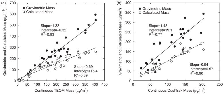
Comparison of gravimetric, calculated, and continuous mass concentrations: (a) TEOM measurement was used at Plants 1 and 2; (b) DustTrak measurement was used at Plant 3. The DustTrak mass concentrations were adjusted with the calculated mass by scenario.

At Plant 1, the average aged particle mass concentrations (i.e., calculated particle mass concentrations) ranged from the lowest of 46.0 μg/m³ for the oxidized scenario (PO) to the highest of 154.9 μg/m³ for the most complex neutralized scenario (PONS). Primary particles (1.0 μg/m³, for the P scenario) accounted for <1% of particle mass for the aged scenarios. Day-to-day and within-day variations in SO₂ and NO_x emissions resulted in substantial variation of the amount of secondary particle formation, as mentioned above. At Plant 2, the pattern of particle mass by scenarios was the same as at Plant 1. The aged particle mass concentrations ranged from 115.5 μg/m³ for the PO scenario to 257.1 μg/m³ for the PONS scenario. Primary particles (1.7 μg/m³) accounted for <1% of total mass for the aged scenarios. During the SCR- off period higher NO concentrations might have resulted in the observed lower ratio of SO₂ to NO_x concentrations and thus less formation of secondary sulfate and aged particles, compared to the SCR-on period. On the other hand, particle number and carbonaceous species showed similar levels regardless of SCR use.

Figure 4b shows relationships between gravimetric, calculated and continuous DustTrak mass concentrations at Plant 3. As for the other plants, the calculated mass was well correlated with the gravimetric mass (R² = .74) and was lower than gravimetric mass. The continuous values from the DustTrak were expected to be a good surrogate of particle mass measurement. However, because light scattering is not a direct measurement of particle mass concentration, the DustTrak values must be corrected using direct particle mass values. The correction factor was determined as the ratio of the calculated particle mass to the averaged DustTrak values. Because the correction factor was expected to vary with particle composition which varied by scenario, it was determined from the ratios for each scenario. The experimentally determined factors were 1.7, 3.9, 6.6, 7.1, 6.8, 3.9, and 7.3 for the P, PO, POS, PONS, OS, O, and S scenarios, respectively. The relationship between the calculated mass and corrected DustTrak mass concentrations for all scenario days is also shown in Figure 4b. The slope was close to unity and the correlation coefficient (R² = .90) was reasonable.

As for Plants 1 and 2, there was a fair amount of day-to-day variation in the aged particle mass concentration at Plant 3. Note, however, that with prior 6-h chamber stabilization, aged particle mass concentrations in exposure atmospheres at all power plants were relatively constant throughout the exposure period on any given day, even though there was substantial variation in SO₂ and NO_x emissions. Although primary particles contributed a small fraction to the aged particle mass concentration at Plants 1 and 2, at Plant 3 primary particle emissions were considerably higher, due possibly to the FGD scrubber (discussed below), as well as to a lower dilution. The aged particle mass concentration averaged by scenario ranged from 43.8 μg/m³ for the control scenario (O) to 173.5 μg/m³ for the PONS scenario. The relative magnitudes for different scenarios at Plant 3 showed the same pattern as at the other two plants. However, at Plant 3 the P scenario contained a relatively higher particle mass concentration (43.2 μg/m³), with a higher number concentration (55,947 particles/cm³), compared to the other plants. Primary particles were composed mainly of sulfate, which was composed mainly of H₂SO₄ and neutralized sulfate, accounting for about 79% of the total mass. The ionic ratio of (H⁺ + NH^{4 +})/(2SO₄ ²⁻ + NO₃ ⁻) ranged from 0.85 to 0.97, with an average of 0.92, which is similar to typical ambient particles with minimal amounts of other salts such as sodium and calcium. The H⁺/SO₄ ²⁻ ratio, indicating relative amount of neutralization, was about 0.72, which means that about 36% of primary sulfate was acidic at this plant. The mass contribution of primary particles to the aged particles was calculated from dilution factors (~12 times, Port A through Port C in Figure 2), primary particle mass concentrations (Port A), and the aged particle mass concentration (Port C) during exposure runs. As a result, primary particles contributed about 8–24% to the total aged particle mass concentrations for the PO, POS, and PONS scenarios, and 115% for the P scenario. An overestimate for the P scenario is likely due to relatively small particle losses that occurred in the pathway to the exposure system.

Particle number and size distribution

It is also worthwhile to compare particle number concentration of the aged particles in the different scenarios. At Plant 1, the highest average was 52,109 particles/cm³ for the neutralized scenario (PONS, which also had the highest aged particle mass concentration), followed by the POS, PO, and P scenarios, with averages of 16,924, 6723, and 1726 particles/cm³, respectively. This pattern was also observed at Plant 2, showing the highest (40,811 particles/cm³) for the PONS scenario, followed by the POS, PO, and P scenarios, with averages of 14,481, 4281, and 910 particles/cm³, respectively. These results suggest that particle number concentration increases with the complexity of scenario, due possibly to increasing particle nucleation.

In addition to primary particle mass concentration, Plant 3 also had a significantly different pattern in particle number concentration. More specifically, the P scenario had a particle number concentration of 55,947 particles/cm³, compared to the first two plants (1726 and 910 particles/cm³ at Plants 1 and 2, respectively). The highest number (69,372 particles/cm³) was for the PO scenario, whereas the lowest (38,483 particles/cm³) was for the neutralized scenario (PONS). Except for the PO scenario (carried out during the last period at this plant), particle number concentration overall decreased inversely with increased scenario complexity, and this could have been a result of increasing particle coagulation with increasing aerosol complexity.

Figure 5 shows the particle size distribution of a typical example of primary particles and aged particles for the PONS scenario at Plants 1 and 2. For primary particles, particle size distribution was monitored using an SMPS plus an APS upstream of the first reaction chamber. The particle size distribution for the aged particles was monitored downstream of the second reaction chamber. The particle size distributions were more or less identical for these two plants. Primary particles were mostly ultrafine particles and had a unimodal distribution with a peak of about 20 nm, whereas the aged particles had a unimodal distribution with a peak of about 100 nm. Overall, the result clearly indicated that the particles grow in size during the aging process.

Figure 5.

Particle size distributions for primary and aged particles at Plants 1 and 2. (See colour version of this figure online at www.informahealthcare.com/iht)

Ionic species

Particulate (total) sulfate for exposure atmospheres was composed mainly of secondary sulfate formed in the first reaction chamber; primary sulfate was negligible at Plants 1 and 2. Total sulfate concentration includes both acidic and neutralized sulfate. Acidic sulfate was calculated from strong acidity (pH) measurement as the equivalent of H₂SO₄ aerosol (Koutrakis et al., 1988). Neutralized sulfate was determined by subtracting acidic sulfate from total sulfate. As expected, all three power plants had similar proportions of the two sulfate species for the same scenario. Day-to-day variation of sulfate within a given scenario contributed significantly to the variation observed in overall aged particle mass concentration.

At Plant 1, the highest total sulfate average was observed for the neutralized scenario (68.2 μg/m³, accounting for 44.0% of the total mass), followed, in order, by the POS and PO scenarios, with averages of 55.8 and 36.1 μg/m³, respectively. The highest acidic sulfate value was 50.2 μg/m³ for the POS scenario, followed by the PO and PONS scenarios, with averages of 27.6 and 14.7 μg/m³, respectively. As expected, neutralized sulfate was present at a higher concentration (53.6 μg/m³) for the neutralized scenario as compared to the unneutralized scenarios (0–8.4 μg/m³). At Plant 2, the highest total sulfate average (154.8 μg/m³, accounting for 62.2% of the total mass) was observed for the neutralized scenario (PONS), followed by the SCR-on POS, PO, and SCR-off POS, with averages of 146.0, 100.3, and 81.5 μg/m³, respectively. The highest acidity sulfate was 107.9 μg/m³ for the SCR-on POS scenario, followed by the PO, SCR-off POS, and PONS scenarios, with averages of 71.6, 68.8, and 15.7 μg/m³, respectively. Acidic sulfate concentrations were higher with lower NO^x emission during the SCR-on period than with higher NO_x emission during the SCR-off period. As expected, neutralized sulfate concentration also showed the highest concentration for the neutralized scenario, 139.1 μg/m³, followed by the SCR-on POS, PO, and SCR-off POS scenarios, with averages of 38.1, 28.8, and 12.9 μg/m³, respectively.

As for the first two plants, at Plant 3 total sulfate concentration for the PONS scenario was the highest (85.0 μg/m³), accounting for 49.0% of the total mass, followed by the POS and PO scenarios, with averages of 83.4 and 77.9 μg/m³, respectively. As expected, the lowest total sulfate concentration was found for the S scenario using particle-free ambient air, instead of stack emissions. For the P scenario, total and neutralized sulfate accounted for 78.7% and 49.1% of the total mass, respectively. Higher concentrations of acidic sulfate were measured for the unneutralized POS (68.9 μg/m³) and PO (66.6 μg/m³) scenarios, which accounted for 47.7% and 80.9% of the total mass, respectively. In addition, lower concentrations of acidic sulfate were observed for the neutralized scenario at this plant compared with Plants 1 and 2 (PONS, 2.5 μg/m³), which demonstrates that most of the H₂SO₄ aerosol was neutralized by the addition of gas-phase NH₃. At all three power plants, addition of gas-phase NH₃ to neutralize H₂SO₄ aerosol for the PONS scenario not only resulted in over five times higher NH^{4 +} concentrations than for the unneutralized scenarios, but also increased particle NO₃ ⁻ concentrations.

Carbonaceous species and secondary organic aerosol

Abnormally high contributions of OC to total particle mass were observed for the primary emissions scenario (P) at all three power plants. These high contributions might have been due to different filter media (Quartz and Teflon filters). A fair amount of artifact OC most likely originated from gas-phase adsorption of VOCs on quartz filters (Mcdow and Huntzicker, 1990; Turpin et al., 1994). Although the source of this VOC is uncertain, it is possible that it may have been due in part to VOCs in ambient air. These could have entered through the purge channel of the parallel plate diffusion denuders and from the addition of particle-free ambient dilution air. A valid statistical comparison of particle OC concentrations with toxicological endpoints requires adjustment for the artifact OC. Toxicological effects are determined from the difference in responses between exposed animals and sham animals (exposed only to particle-free air). It was thus decided to subtract a background OC level to correct the measured OC concentrations for all scenarios. At Plants 1 and 2, the OC concentrations for the P scenario were chosen as the most suitable background value because the total mass (1.0 and 1.7 μg/m³, respectively) was negligible. At Plant 3, the OC concentration for the control oxidized scenario (O) was chosen as the background OC value because it was the lowest value of all scenarios at this plant. The OC concentrations presented in Tables 5–7 are net values reflecting subtraction of this background OC level. These values are different from the unadjusted values reported previously for Plant 1 (Ruiz et al., 2007a).

At all three power plants, the amount of OC formed was determined by the type of scenario. The S code represents adding α-pinene (and ozone) into the second reaction chamber to produce SOA. At Plant 1, after adjustment for background OC, the POS and PONS scenarios had significant amounts of OC, with averages of 51.6 and 53.6 μg/m³, respectively. At Plant 2, inadvertently more than the routine amount of α-pinene was used for the first 2 days of the SCRoff POS scenario, which led to abnormally high OC, particle number, and mass concentrations. As for Plant 1, the SCR-on POS and PONS scenarios showed significant amounts of OC, with averages of 59.0 and 35.1 μg/m³, respectively. At Plant 3, particulate OC concentrations for the POS, PONS, OS, and S scenarios ranged from 52.0 to 83.6 μg/m³, which are substantially higher than those for the P, PO, and O scenarios (0–1.9 μg/m³), all of which lack SOA.

Particulate EC concentrations at the first two power plants were low, with a high variability: 0–11.9 μg/m³ at Plant 1 and 1.7–12.5 μg/m³ at Plant 2. Concentrations were lowest in the P scenarios (Tables 5 and 6), but with aging and addition of SOA, EC increased, suggesting that a portion of this is likely artifactual and representative of pyrolyzed OC erroneously reported as EC (Birth, 1998; Yu et al., 2002). The variability is also likely due to a fair amount of day-to-day variation in primary emissions. In McDonald et al. (2010), EC comprised 10% of the ash, which in turn comprised 1% of the total mass of the lab-based exposure atmosphere. This corresponded to less than 1 μg/m³, a value substantially lower than at these plants. On the other hand, EC at Plant 3 was not detected for any of the scenarios. It has been reported that a wet FGD scrubber can remove some of the primary particles that penetrated through the ESP, and the scrubber itself is not a source for EC emissions (Meij, 1994; US DOE, 2003). Thus, the absence of EC at Plant 3 is likely due to a high collection efficiency of primary particles by the combined ESP and FGD scrubber.

Table 6.

Particle component concentrations at Plant 2.

			POS
Species	P(n = 4)a	PO(n = 4)	Non-SCR (n = 4)	SCR (n = 8)	All (n = 12)	PONS(n = 4)
Particle mass (μg/m3)b	1.7 ± 1.8c	115.5 ± 18.5	213.6 ± 60.2	212.1 ± 39.7	212.7 ± 45.1	257.1 ± 10.0
Gravimetric mass (μg/m3)	1.9 ± 1.3	224.3 ± 53.3	377.2 ± 100.0	432.5 ± 95.0	414.1 ± 96.0	477.7 ± 51.6
Continuous mass (μg/m3)d	13.9 ± 9.5	202.9 ± 36.7	201.3 ± 49.8	308.1 ± 59.7	279.0 ± 74.0	354.8 ± 37.7
Number (particles/cm3)	910 ± 964	4281 ± 1911	22,500 ± 19,085	11,473 ± 3774	14,481 ± 10,457	40,811 ± 2179
Total sulfate (μg/m3)	0.0 ± 0.0	100.3 ± 16.3	81.5 ± 29.0	146.0 ± 36.7	122.6 ± 46.1	154.8 ± 12.4
Acidic sulfate (μg/m3)e	0.0 ± 0.0	71.6 ± 17.0	68.8 ± 22.0	107.9 ± 31.7	93.7 ± 33.7	15.7 ± 3.8
Neutralized sulfate (μg/m3)f	0.0 ± 0.0	28.8 ± 1.3	12.9 ± 10.7	38.1 ± 12.0	28.9 ± 16.8	139.1 ± 15.5
Nitrate (μg/m3)	0.0 ± 0.0	0.2 ± 0.2	0.8 ± 0.2	0.3 ± 0.3	0.5 ± 0.3	6.4 ± 1.7
Ammonium (μg/m3)	0.0 ± 0.0	6.1 ± 0.4	4.7 ± 1.2	9.1 ± 3.4	7.5 ± 3.5	50.3 ± 5.3
OC (μg/m3)	0.0 ± 0.0	0.0 ± 0.0	114.3 ± 71.6	59.0 ± 20.2	81.2 ± 52.5	35.1 ± 10.1
EC (μg/m3)	1.7 ± 1.8	7.3 ± 3.2	10.8 ± 3.9	12.5 ± 6.9	11.9 ± 6.0	10.2 ± 3.9
Na (ng/m3)	0.0 ± 0.0	2.5 ± 4.9	1.3 ± 1.9	0.0 ± 0.0	0.3 ± 0.8	0.0 ± 0.0
Mg (ng/m3)	2.1 ± 2.4	0.8 ± 1.6	2.3 ± 3.2	0.0 ± 0.0	0.5 ± 1.4	0.1 ± 0.1
Al (ng/m3)	0.2 ± 0.5	2.8 ± 2.8	2.7 ± 1.6	2.2 ± 2.4	2.3 ± 2.2	0.2 ± 0.4
Si (ng/m3)	1.5 ± 1.5	8.1 ± 14.3	4.2 ± 0.7	2.5 ± 2.4	2.9 ± 2.2	1.2 ± 0.5
P (ng/m3)	0.0 ± 0.0	4.3 ± 8.5	0.1 ± 0.2	0.7 ± 1.6	0.6 ± 1.4	0.0 ± 0.0
S (μg/m3)	0.0 ± 0.0	33.4 ± 5.4	27.2 ± 9.7	48.7 ± 12.2	40.9 ± 15.4	51.6 ± 4.1
K (ng/m3)	0.2 ± 0.4	0.1 ± 0.2	0.3 ± 0.2	0.0 ± 0.1	0.1 ± 0.1	0.2 ± 0.2
Ca (ng/m3)	0.1 ± 0.2	0.3 ± 0.4	0.4 ± 0.5	0.7 ± 1.2	0.6 ± 1.0	0.2 ± 0.3
Ti (ng/m3)	0.1 ± 0.2	0.1 ± 0.1	0.2 ± 0.2	0.2 ± 0.1	0.2 ± 0.1	0.1 ± 0.1
Cr (ng/m3)	0.1 ± 0.2	0.0 ± 0.0	0.0 ± 0.0	21.2 ± 33.7	17.0 ± 31.0	2.2 ± 3.6
Fe (ng/m3)	3.4 ± 3.9	0.2 ± 0.3	0.0 ± 0.0	175.3 ± 270.4	140.2 ± 249.6	16.8 ± 30.1
Ni (ng/m3)	0.0 ± 0.1	0.0 ± 0.0	0.2 ± 0.1	17.9 ± 28.1	14.3 ± 25.8	1.8 ± 3.5
Zn (ng/m3)	0.0 ± 0.1	0.1 ± 0.1	0.0 ± 0.0	0.1 ± 0.2	0.1 ± 0.2	0.0 ± 0.0
Se (ng/m3)	0.1 ± 0.3	0.4 ± 0.5	0.0 ± 0.0	0.1 ± 0.2	0.1 ± 0.2	0.2 ± 0.3
Pb (ng/m3)	0.5 ± 1.1	0.1 ± 0.1	0.0 ± 0.0	0.1 ± 0.2	0.1 ± 0.2	0.6 ± 0.7

^aNumber of days.

^bParticle mass was estimated from the sum of analyzed components.

^cAll values are average ± standard deviation.

^dContinuous mass was determined using a TEOM monitor.

^eH₂SO₄ equivalent.

^fTotal sulfate - H₂SO₄

A subset of particulate SOA species collected on Teflon filters was measured using GC-MS method. Several representative filters were selected; two and one each from the POS and PONS scenarios at Plants 1 and 2, respectively. This analysis was not conducted at Plant 3 as the pattern was expected to be similar to the previous two plants. Three field blanks were also analyzed to correct for background. Seven SOA species were identified (Table 8). At Plant 1, cis-pinic acid was the dominant species for both scenarios, accounting for about 90% of total SOA species. At Plant 2, the dominant species were cis-pinic acid (about 70% of total SOA species) and pinolic acid (about 20% of total SOA species). On the other hand, pinonaldehyde, cis-nor-pinic acid, pinalic acid, transnor- pinic acid, cis-pinic acid, and trans-pinic acid were minor species at both power plants and scenarios. All these species are typical SOA products of α-pinene (Kanakidou et al., 2005). The sum of the identified SOA species varied considerably and accounted for 50–107% of the corresponding OC concentrations measured by TOR analytical method. The difference might have resulted from analytical or sampling errors due to different filter media (Quartz and Teflon filters) or from different environmental conditions (e.g., relative humidity and temperature). However, the composition of the identified SOA species was relatively similar for the two power plants at which they were measured.

Table 8.

Selected SOA species at Plants 1 and 2.

	Plant 1a		Plant 2
Species	POS(n = 2)b	PONS(n = 2)	POS(n = 1)	PONS(n = 1)
Pinonaldehyde	298 (1.0)c	590 (3.5)	1218 (3.5)	792 (2.6)
Pinalic acid	137 (0.5)	42 (0.2)	1009 (2.9)	242 (0.8)
Trans-nor-pinic acid	560 (1.9)	404 (2.4)	453 (1.3)	515 (1.7)
Cis-pinonic acid	98 (0.3)	110 (0.6)	808 (2.3)	888 (2.9)
Cis-pinic acid	27,102 (89.8)	15,448 (90.7)	23,099 (66.4)	21,414 (70.9)
Trans-pinic acid	376 (1.2)	212 (1.2)	241 (0.7)	155 (0.5)
Pinolic acid	1600 (5.3)	232 (1.4)	7964 (22.9)	6196 (20.5)
Total SOA species	30,171	17,038	34,792	30,202
Organic carbon	60,934	16,903	32,441	37,185
Total %d	50%	101%	107%	81%

^aRuiz et al., 2007a.

^bNumber of samples.

^cConcentration is ng/m³ with % fraction of species to total SOA in parentheses.

^dTotal % of SOA species to corresponding OC concentration.

Elemental composition

Elemental concentrations are summarized by scenario in Tables 5–7. Two times the uncertainty of each XRF measurement was used as the method detection limit (MDL) for each element. Initially, XRF analysis was performed with filter samples collected from the exposure atmospheres. However, these results showed very few elements above their respective MDLs. This was due to the high dilution ratios (a total factor of 1000–2000) between the stack emissions and the exposure atmospheres, coupled with relatively low elemental concentrations in the stack emissions. To overcome this limitation, XRF analysis was subsequently performed for primary particles collected upstream of the first reaction chamber (Port A). The elemental composition of aged particles used for exposure atmospheres was estimated using the dilution factors of Port A through Port C. Sulfur concentrations were independently determined from sulfate concentrations by IC because sulfur is expected to be dominated by secondary sulfate formed and IC sulfate is more reliable than XRF sulfur.

From Table 5 (Plant 1) and Table 6 (Plant 2), a total of 15 elements were identified. Except for sulfur, they were all present at low concentrations. On average, the sum of elements except sulfur account for about 0.1% of the aged particle mass concentration. Elemental concentrations also varied significantly. At Plant 2, in particular, substantially higher concentrations of Cr, Fe, and Ni were observed for 3 days (July 13, September 7 and 8, 2005) of the SCR-on POS scenario days, compared to the other scenarios. A slight elevation in these elements was also observed for 1 day at Plant 1 (November 5, 2004). On these days primary particle concentrations also increased by a factor of 17, compared to the other days. The episode of high Cr, Fe, and Ni concentrations are discussed in detail below. Selenium (Se), an element as a tracer for coal-fired power plant emissions in source apportionment studies (e.g., Thurston and Spengler, 1985), was present at concentrations less than detection limits, due to very low primary particle mass concentrations (1–2 μg/m³) present.

Overall, Al, Si, S, Ca, and Fe were the most abundant elements, relative to other elements, at Plant 1. At Plant 2, Al, Si, and S were the most abundant elements present in the exposure atmospheres, except for the 3 days with higher levels of Cr, Fe, and Ni. These elements are common elements resulting from coal combustion process. Furthermore, the relatively higher amount of Ca at Plant 1 is most likely due to the use of Ca-rich subbituminous coal. In general, coals contain significant amounts of Al, Si, Fe, Ca, and Mg in the form of primarily quartz (SiO₂), kaolin (Al₂Si₂O₅[OH]₄), pyrite (FeS₂), calcite (CaCO₃), or dolomite (MgCa[CO₃]₂). In addition, trace elements in coal undergo complex physical and chemical transformations in the boiler in the process of forming particles. They are vaporized in a high temperature boiler, and as the temperature decreases upstream of the ESP, the elements can nucleate and/or condense onto existing particles (Quann et al., 1990; US DOE, 2003).

At Plant 3 (Table 7), the relative variability of the concentrations was significantly lower than that observed for the other two plants. Most elemental concentrations present in the table were above the MDL values. The abundant elements included Na, Mg, Al, P, S, Fe, and Se for this plant, which was generally different from those for Plants 1 and 2. In addition, the sum of elements (excluding S) corresponded on average to 0.4% of the aged particles, which was higher than that at Plants 1 and 2.

The following may help to explain why the primary particles had a different elemental composition at Plant 3. Although the wet FGD scrubber is expected to remove some of primary particles including trace elements, it is also expected to be a source of stack emission particles (Meij, 1994; US DOE, 2003; Srivastava et al., 2004). Meij (1994) reported that fly dust downstream of wet FGD scrubbers were composed of 40% fly ash, 10% gypsum (CaSO₄·2H₂O), and 50% evaporated droplets saturated with gypsum. However, primary particle composition at Plant 3 was some-what different from the compositions reported previously. This is most likely because of different particle sizes between two studies; primary particles at Plant 3 are expected to be the smaller sizes (presumably submicron size). Srivastava et al. (2004) also described the formation and emissions of submicron H₂SO₄ aerosol by wet FGD scrubbing in coal-fired power plants.

The removal efficiency of ESPs increases with particle size. Although the overall removal efficiency of the ESP is about 99% (of overall particle mass), it is considerably less efficient for submicron particles (0.1–1.0 μm), which are more highly enriched in condensed trace elements (Quann et al., 1990; US EPA, 1993; Meij, 1994). At Plant 3, the overall removal efficiency through the combination of an ESP and a wet FGD scrubber would likely be greater than by an ESP alone because the wet FGD scrubber is expected to remove some particles. On the other hand, the wet scrubbing process is likely to be a source of particles. The finding that a major component of the primary particles down-stream of the scrubber was sulfate (composed mainly of H₂SO₄ and NH₃-neutralized sulfate), accounting for 79% of the total mass, supports this hypothesis. This composition also suggests that primary particles at Plant 3 fell primarily in the submicron size range because sulfate is typically found in this size range in both ambient air (Koutrakis and Kelly, 1993; Hazi et al., 2003) and power plant emissions (Srivastava et al., 2004). Consequently, most of the primary particles at Plant 3 were likely derived from the wet scrubbing rather than from coal combustion.

The wet FGD scrubber used was an inhibited oxidation system, which means that thiosulfate (or elemental S) was added to prevent the formation of CaSO₄·2H₂O (predominately, CaSO₃·1/2H₂O) in a co-current absorber tower. A small amount of sodium formate (NaCOOH) was also added to buffer the pH drop through the absorber and enhance SO₂ removal. Thus it is possible that Na, the most abundant element after sulfur, results from aerosolization of sodium salts in the wet scrubber. Furthermore, selenium (Se) was present at relatively high concentrations at the plant. As Se is a volatile element, it is typically present in vapor phase in stack emissions and its behavior is complex in power plant emissions (EPRI, 2008). It is also found in both fly ash and flue gas, and a substantial amount of Se is not removed by the ESP.

Even though limestone particles containing substantial amounts of Ca are used by the wet FGD scrubber, relatively low concentrations of Ca (6.7–14.8 ng/m³) were found in the exposure atmosphere. It is likely that the particle sizes that passed through the stack extraction system at Plant 3 were within the submicron range, as for the other two plants. On the other hand, calcium sulfate formed in the FGD scrubbing process is an abrasive, sticky, and compressible material and is composed primarily of finely divided crystals ranging from 1 to 250 μm. When FGD scrubbers using limestone were tested with both low-sulfur and high-sulfur coals, less Ca was found in the flue gas downstream of the scrubber for high-sulfur coal combustion (US DOE, 2003). These processes could explain the relatively low amounts of Ca found in the scrubbed stack gas, and consequently, the Ca in the exposure atmospheres could have been mostly from the smaller particles (relatively inefficiently removed by the ESP) that were present in the flue gas due to the combustion of coal, rather than from the limestone.

High Cr, Fe, and Ni episodes

It is important to address the high content of these elements mentioned above. Coals contain significant amounts of Al, Si, Fe, Ca, and Mg; however, Cr and Ni are typically found in only trace amounts. Relatively high amounts of Cr and Ni in relation to primary elemental constituents might have been due to (1) a foreign, non-coal source, such as corrosion, and (2) coal with a much higher-than-normal Cr and Ni content. The latter might be supported by the fact that Plant 2 used bituminous coals derived from various regions.

High Cr and Ni concentrations were also observed from in-stack measurements performed prior to animal exposure experiments at Plant 2. As part of the study, preliminary in-stack tests were conducted to investigate primary particle mass and elemental composition at both Plants 1 and 2, during October 19–24, 2004, and December 13–14, 2004, respectively. Several fine particle samples were collected for 20 min to 3 h on quartz filters with a 2.5-μm cut-off cyclone inside the stack without dilution, and then analyzed for gravimetric mass and elemental concentrations. This test was conducted in accordance with the EPA Conditional Method 040 (US EPA, 2002). Figure 6 shows mass contributions of selected elements to in-stack particle mass concentrations at Plants 1 and 2. In this figure, elements associated with coal combustion (Al, S, Ca, Ti, and Se) are shown in addition to Cr, Fe, and Ni. Si was not available because of the quartz filter media used.

Figure 6.

Weight % of selected elements to in-stack particle mass concentrations at Plants 1 and 2.

At Plant 1, the selected elements clearly varied together; moreover, there was no elevation of Cr and Ni. Ca was the most abundant element, accounting for about 20% of the total mass, which was consistent with exposure atmospheres at this power plant. On the other hand, at Plant 2 some of the in-stack samples indicated elevated Cr, Fe, and Ni concentrations consistent with those observed on the 3 “high” days during the exposure runs. Averaged mass contributions of Cr, Fe, and Ni to the in-stack particle mass were 3.4%, 8.9%, and 1.2%, respectively, with two samples (Samples 1 and 3) having substantially higher Cr and Ni concentrations. In Sample 1, the mass contributions of all elements were elevated altogether, whereas in Sample 3 only Cr and Ni fractions were increased without the concomitant elevation of Fe. Because contamination by corrosion is expected to result in elevations of Cr, Fe, and Ni together, regardless of other elements, this result suggests that the elevated Cr and Ni in these samples is not likely to have been influenced by corrosion.

It is also expected that any oxidized corrosion particles that may have been aerosolized by mechanical processes would predominantly exist in greater-than-submicron size ranges. At the same time, only relatively much smaller particles pass through the ESP with reasonable efficiency, although some larger particles may escape collection. In order to identify single particle size and composition, scanning electron microscope (SEM) analysis was performed for the primary particles collected at Port A for days with both high and low elemental concentrations. An uncoated slice of each of the eight collected filters was placed on a 25-mm Zeiss SEM stub and then examined with a LEO 1450VP scanning electron microscope (Carl Zeiss SMT, Thornwood, NY) at 15 KeV using a magnification of 2000 times. The X-ray analysis was performed with an Inca300/SEM Si (Li) X-ray detector (Oxford Instruments, Concord, MA). From the SEM analyses, the particle sizes were generally submicron particles with a spherical shape. Particles that had substantially higher Cr, Fe, and Ni content were in a similar size (submicron) range to those that contained less of these elements. These elements were also observed generally together on a single particle. This result suggests that the spherical, submicron particles with high Cr, Fe, and Ni content are more likely due to the combustion process, rather than a result of corrosion. However, we are unable to resolve this issue with certainty because of somewhat conflicting information regarding the source of the elevated Cr, Fe, and Ni on certain days.

Comparison of the results among coal-fired power plants

In this section, we compare the physical and chemical properties of the aged particles used for toxicological studies from all three power plants. Particle mass, number, total sulfate, acidic sulfate, neutralized sulfate, and organic carbon are compared in Figure 7.

Figure 7.

Particle component concentrations at the three power plants: The averages with standard deviations (error bars) are shown for each scenario from each of the different plants. (See colour version of this figure online at www.informahealthcare.com/iht)

Of the plants studied, primary particles at Plant 3 contributed somewhat to the aged particle mass concentrations. Figure 7 also shows that the primary particles consisted mostly of H₂SO₄ and NH₃-neutralized sulfate; this is likely a result of emissions from the wet FGD scrubber. On the other hand, at Plants 1 and 2 the primary particle mass concentrations were too low to estimate their composition. For all power plants, the aged particle mass concentrations increased with the complexity of scenario, with the highest values for the most complex, neutralized scenario (PONS), followed by POS, PO, and P scenarios. Furthermore, particle number concentrations at the first two power plants increased with scenario complexity, which suggests that nucleation of H₂SO₄ and SOA was a dominant mechanism of particle formation. In contrast, at Plant 3 particle number concentration decreased somewhat with scenario complexity, which suggests that coagulation was a dominant mechanism of particle formation.

The major components of the aged particles are total sulfate composed of acidic (H₂SO₄) and neutralized sulfate (ammonium sulfate, letovicite, or ammonium bisulfate). Of the three plants studied, Plant 2 had the highest particle mass and sulfate concentrations in the aging scenarios. It was most likely due to the higher ratio of SO₂ to NO_x emissions, due to the use of a SCR for NO_x emission control without SO₂ scrubbing. This was also confirmed with higher sulfate during the SCR-on period than during the SCR-off period. Overall, total sulfate accounted for between 38% and 95% of the aged particle concentrations for the three power plants: H₂SO₄ aerosol accounted for about 1–81% and neutralized sulfate accounted for about 5–54% of the aged particles.

OC concentrations exhibited similar patterns at all three power plants. The OC level depended primarily on whether α-pinene was added to simulate atmospheric production of SOA (scenarios with S code). The POS and PONS scenarios thus had more OC, as well as higher particle mass concentrations, than the other scenarios. Overall, OC accounted for about 14–54% of the aged particle mass concentrations. Previous studies have reported that organic compounds represent about 20–50% of the ambient fine particle mass at continental mid-latitudes (Saxena and Hildemann, 1996; Putaud et al., 2004). In contrast to major components, the contribution of trace elements to the aged particle mass concentrations was very low because of the use of ESPs at all three coal-fired power plants.

Comparison with ambient environments

In order to provide additional context for the toxicological effects documented in the companion TERESA papers, it was of interest to compare the TERESA exposure atmospheres with ambient particles. In particular, our research group has conducted many studies of concentrated ambient particles (CAPs) collected in Boston, and has a rich data set. It is important to note that we would not expect the TERESA exposure atmospheres to be similar to the ambient environment. Although the TERESA scenarios simulated atmospheric reactions of coal-fired power plant emissions, ambient particles are comprised of constituents from multiple sources, including mobile sources, oil-fired power plants, and a variety of industrial emissions. In addition, both biogenically and anthropogenically derived SOA is not limited to α-pinene as a VOC precursor in ambient air, unlike in the TERESA scenarios. However, it is of interest to determine how closely (or disparately) the TERESA atmospheres compare to typical ambient environments.

For the purposes of this comparison, we selected the PONS scenario, as it was expected to be most representative of human exposure. This is because it contains oxidized SO₂, partially neutralized sulfate, and secondary organic aerosol that would be expected to associate with particles formed downwind of the plant. The TERESA PONS exposures were compared to those reported in several CAPs studies, primarily in Boston (Clarke et al., 2000; Batalha et al., 2002; Gurgueira et al., 2002; Wellenius et al., 2003, 2004), but also in Chapel Hill, NC (Kodavanti et al., 2005) and Fresno, CA (Smith et al., 2003). The concentrations of major particle constituents at each of the three power plants are compared to CAPs in Table 9.

Table 9.

Comparison with CAPs compositions.

Parameter	Plant 1 (PONS, n = 12a)	Plant 2 (PONS, n = 4)	Plant 3 (PONS, n = 4)	Boston CAPs studiesb	Fresno CAPs studyc	Chapel Hill CAPs studyd
Particle mass (μg/m3)	155	257	174	333	475	1172
Sulfate (μg/m3)	68 (44%)	155 (60%)	85 (49%)	71 (21%)	29 (6.1%)	338 (29%)
OC (μg/m3)	30 (19%)	35 (14%)	52 (30%)	75 (23%)	95 (20%)	287 (24%)
EC (μg/m3)	5 (3.2%)	10 (3.9%)	0 (0%)	18 (5.4%)	17 (4%)	17 (1.5%)
Particle number (particles/cm3)	52,100	40,800	38,500	44,000	110,000	—e
Sum of elementsf (μg/m3)	0.03 (0.02%)	0.02 (0.01%)	0.3 (0.2%)	26 (7.8%)	20 (4.2%)	2.8 (0.2%)
Na (μg/m3)	0.000	0.000	0.093	5.0	—	—
Mg (μg/m3)	0.001	0.000	0.013	—	—	—
Al (μg/m3)	0.004	0.000	0.010	1.8	3.0	1.6
Si (μg/m3)	0.004	0.001	0.001	6.5	8.3	—
P (μg/m3)	0.001	0.000	0.058	—	—	—
S (μg/m3)	23	52	28	32	6.7	—
K (μg/m3)	0.000	0.000	0.001	2.0	2.2	—
Ca (μg/m3)	0.016	0.000	0.007	3.4	2.4	—
Ti (μg/m3)	0.001	0.000	0.001	0.4	0.3	—
Cr (μg/m3)	0.000	0.002	0.007	0.02	—	—
Fe (μg/m3)	0.003	0.017	0.044	6.0	3.3	—
Ni (μg/m3)	0.000	0.002	0.003	0.1	0.01	0.03
Zn (μg/m3)	0.000	0.000	0.004	0.6	0.5	1.0
Se (μg/m3)	0.000	0.000	0.019	0.03	0.01	—
Pb (μg/m3)	0.000	0.001	0.000	0.3	0.1	0.2

^aNumber of samples.

^bAveraged concentrations reported by Clarke et al., 2000; Batalha et al., 2002; Gurgueira et al., 2002; Wellenius et al., 2003; Wellenius et al., 2004.

^cAverage concentrations reported by Smith et al., 2003.

^dAverage concentrations reported by Kodavanti et al., 2005.

^eNot available.

^fSum of elemental concentration excluding sulfur.

Particle mass and OC concentrations were lower in our study compared to CAPs, whereas sulfate concentrations were generally comparable or higher, with the exception of Chapel Hill CAPs, which were very high in sulfate. Note that sulfate in our study simulated not only primary sulfate emissions from the power plants but also secondary sulfate formation from SO₂ emitted from coal-fired power plants during transport. Particle number concentrations were roughly similar in our study compared with CAPs, except for Fresno CAPs, which were present in significantly higher numbers. Elemental carbon was present at lower concentrations in TERESA than in CAPs, which would be expected given the low EC emissions from power plants and the significant contribution of mobile sources to CAPs in urban areas. All of the individual elemental concentrations in our exposure scenarios were substantially lower than those reported in CAPs studies, with the exception of Cr, which at Plant 3 was about 35% of the Cr in Boston CAPs, and Se, which at Plant 3 was 76% of that in Boston CAPs. As a result, the total contribution of measured elements to mass was much lower in TERESA (0.01–0.2%) than in CAPs studies (0.2–7.9%). The comparison with ambient CAPs suggests that sulfate derived from coal-fired power plant emissions contributes significantly to ambient particles, whereas the elemental contribution is substantially less.

Acidic sulfate in TERESA atmosphere was compared to that in ambient particles because the acidity was not available in CAPs studies. Acidic sulfate concentrations in the TERESA PONS atmospheres, 14.7 μg/m³ at Plant 1, 15.7 μg/m³ at Plant 2, and 2.5 μg/m³ at Plant 3, were substantially higher than in ambient particles, 0.48 μg/m³ and 1.77 μg/m³ in St. Louis, MO, and Eastern Tennessee, respectively (Dockery et al., 1992) and 0.88 μg/m³ in Atlanta, GA (Peel et al., 2005), which are both affected by regionally transported power plant emissions. However, on a total mass basis, acidic sulfate in the TERESA PONS atmospheres contributed 9.5%, 6.1%, and 1.4% at Plants 1, 2, and 3, respectively, which are comparable to 2.7% in St. Louis, 8.4% in Eastern Tennessee, and 4.6% in Atlanta.

Conclusions

The physical and chemical properties of primary and aged particles derived from stack emissions were estimated under different typical simulated atmospheric scenarios at three pulverized coal-fired power plants. The mobile laboratory system designed successfully simulated the atmospheric transformations that emissions undergo in a plume during transport in the atmosphere. Stack emissions were diluted by a total factor of about 1000–2000 to simulate the diffusion of the plume when it reaches the receptor after a transport time of 24–36 h.

Aged particle mass concentrations varied by scenario and plant, ranging from 43.8 to 257.1 μg/m³. The highest concentrations were for the most complex scenario (primary particles + secondary sulfate + NH³ neutralization + secondary organic aerosol). This scenario is considered to be the most representative of urban areas downwind of coal-fired power plants. Our results indicate that the secondary sulfate (as well as aged particle mass) concentrations depend on the ratio of SO₂ and NO emissions, which, in turn, depend on the type of coal and emissions control devices.

All three coal-fired power plants used ESPs, but Plant 3 also used a wet FGD scrubber, and emissions from this plant had substantially higher primary particle mass (47.8 mg/m³, as compared to about 1.0 mg/m³ at the other plants) and number concentrations than those from the other plants. At Plant 3, primary particles were composed primarily of sulfate (primarily H₂SO₄ and NH₃-neutralized sulfate), accounting for about 79% of the total mass, and about 36% of the sulfate was acidic. These particles probably originated primarily from the wet scrubbing process, rather than from the coal combustion process.

At all three coal-fired power plants, sulfate and organic carbon (OC) were major components of the aged particles, whereas the contributions of trace elements (derived from primary particles) were very low as compared to urban ambient particles. This may suggest that sulfate derived from coal-fired power plant emissions contributes significantly to ambient particles, whereas the elemental contribution is substantially lower. This is not unexpected, given the use of primary particle controls (primarily ESPs) on US power plants. Overall, physical and chemical properties of aged particles appear to be influenced by coal type, emissions controls, and the particular atmospheric scenarios employed.

Table 3.

Gaseous species concentrations and metrological parameters for each scenario at Plant 2.^a

			POS
Species	P(n = 4)b	PO(n = 4)	Non-SCR(n = 4)	SCR(n = 8)	All(n = 12)	PONS(n = 4)
O3(ppb)	0.0 ± 0.0c	13.5 ± 1.9	29.6 ± 9.8	17.5 ± 13.8	21.5 ± 13.5	19.0 ± 2.1
NO (ppb)	5.5 ± 1.8	8.4 ± 3.0	1.3 ± 0.4	5.5 ± 2.4	4.1 ± 2.8	6.5 ± 1.0
NO2(ppb)	2.1 ± 0.5	2.2 ± 4.3	0.4 ± 0.5	0.7 ± 1.2	0.6 ± 1.0	0.1 ± 0.1
SO2(ppb)	34.3 ± 12.0	37.0 ± 3.5	36.0 ± 3.0	30.8 ± 7.3	32.5 ± 6.5	25.7 ± 2.2
HNO3(ppb)	0.2 ± 0.1	0.9 ± 0.5	1.2 ± 0.1	0.4 ± 0.1	0.6 ± 0.4	1.1 ± 0.5
HONO (ppb)	2.9 ± 2.2	1.9 ± 0.6	4.5 ± 0.9	2.1 ± 1.2	2.9 ± 1.6	2.2 ± 1.2
NH3(ppb)	0.1 ± 0.2	0.0 ± 0.0	3.2 ± 3.3	15.4 ± 23.3	11.3 ± 19.6	1.9 ± 2.2
Formaldehyde (ppb)	NMd	NM	20.7 ± 2.8	11.8 ± 6.7	14.7 ± 7.1	10.7 ± 7.3
Acetaldehyde (ppb)	NM	NM	6.8 ± 1.1	4.2 ± 1.5	5.0 ± 1.9	5.7 ± 1.9
Acetone (ppb)	NM	NM	22.6 ± 2.9	10.0 ± 7.1	14.2 ± 8.6	20.5 ± 4.5
α-Pinene (ppb)	NM	NM	7.8 ± 8.0	6.2 ± 4.2	6.8 ± 5.4	6.0 ± 3.4
Temp. (°C)	24.2 ± 0.1	22.7 ± 1.2	23.3 ± 1.1	22.7 ± 0.9	22.9 ± 0.9	23.1 ± 0.7
RH (%)	58.2 ± 1.8	37.7 ± 4.4	70.4 ± 34.6	52.4 ± 20.7	58.4 ± 26.1	50.7 ± 2.4

^aVOCs were not measured for the non-SOA scenarios, P and PO, but the concentrations were expected to have been close to typical ambient levels, resulting from relatively high dilution with particle-free ambient air, required to supply the exposure atmospheres and characterization measurements.

^bNumber of days.

^cAverage ± standard deviation.

^dNot measured.

References

- Annual Energy Review. Energy Information Administration, DOE/EIA- 0384 2006 [Google Scholar]
- Batalha JRF, Saldiva PHN, Clarke RW, Coull BA, Stearns RC, Lawrence J, Murthy GGK, Koutrakis P, Godleski JJ. Concentrated ambient air particles include vasoconstriction of small pulmonary arteries in rats. Environ Health Perspect. 2002;110:1191–1197. doi: 10.1289/ehp.021101191. [DOI] [PMC free article] [PubMed] [Google Scholar]
- Chen LC, Lam HF, Kim EJ, Guty J, Amdur MO. Pulmonary effects of ultrafine coal fly ash inhaled by guinea pigs. J Toxicol Environ Health. 1990;29:169–184. doi: 10.1080/15287399009531381. [DOI] [PubMed] [Google Scholar]
- Chen X, Hopke PK. Secondary organic aerosol from α-pinene ozonolysis in a dynamic chamber system. Indoor Air. 2009;19:335–345. doi: 10.1111/j.1600-0668.2009.00596.x. [DOI] [PubMed] [Google Scholar]
- Chow JC, Watson JG, Kuhns H, Etyemezian V, Lowenthal DH, Crow D, Kohl SD, Engelbrecht JP, Green MC. Source profiles for industrial, mobile and area sources in the Big Bend Regional Aerosol Visibility and Observational study. Chemosphere. 2004;54:185–208. doi: 10.1016/j.chemosphere.2003.07.004. [DOI] [PubMed] [Google Scholar]
- Clarke RW, Coull B, Reinisch U, Catalano P, Killingsworth CR, Koutrakis P, Kavouras I, Murthy GGK, Lawrence J, Lovett E, Wolfson JM, Verrier RL, Godleski JJ. Inhaled concentrated ambient particles are associated with hematologic and bronchoalveolar lavage changes in caniners. Environ Health Perspect. 2000;108:1179–1187. doi: 10.1289/ehp.001081179. [DOI] [PMC free article] [PubMed] [Google Scholar]
- Diaz E, Lemos M, Coull B, Long M, Ruiz P, Gupta T, Kang CM, Godleski JJ. Toxicological Evaluation of Realistic Emission Source Aerosols (TERESA) Assessment of Breathing Pattern. 2011;23(S2):42–59. doi: 10.3109/08958378.2010.578169. [DOI] [PMC free article] [PubMed] [Google Scholar]
- Dockery DW, Schwartz J, Spengler JD. Air pollution and daily mortality: Associations with particulates and acid aerosols. Environ Res. 1992;59:362–373. doi: 10.1016/s0013-9351(05)80042-8. [DOI] [PubMed] [Google Scholar]
- Dockery DW, Pope A, Xu X, Spengler JD, Ware JH, Fay ME, Ferris BG, Speizer FE. An association between air pollution and mortality in six U.S. cities. N Engl J Med. 1993;329:1753–1759. doi: 10.1056/NEJM199312093292401. [DOI] [PubMed] [Google Scholar]
- Dormans JA, Steerenberg PA, Arts JH, van Bree L, de Klerk A, Verlaan AP, Bruijntjes JP, Beekhof P, van Soolingen D, van Loveren H. Pathological and immunological effects of resirable coal fly ash in male Wistar rats. Inhal Toxicol. 1999;11:51–69. doi: 10.1080/089583799197267. [DOI] [PubMed] [Google Scholar]
- Electric Power Research Institute. Multimedia Fate of Selenium and Boron at Coal-Fired Power Plants Equipped with Particulate and Wet FGD Controls. Report 1015615. Palo Alto, CA: Electric Power Research Institute; 2008. [Google Scholar]
- Gilmour MI, O’Conner S, Dick CA, Miller CA, Linak WP. Differential pulmonary inflammation and in vitro cytotoxicity of size-fractionated fly ash particles from pulverized coal combustion. J Air Waste Manage Assoc. 2004;54:286–295. doi: 10.1080/10473289.2004.10470906. [DOI] [PubMed] [Google Scholar]
- Godleski JJ, Koutrakis P, Kang CM, Diaz E, Rohr AC. Toxicological Evaluation of Realistic Emission Source Aerosols (TERESA) Introduction and overview. 2011a;23(S2):1–10. doi: 10.3109/08958378.2010.568019. [DOI] [PMC free article] [PubMed] [Google Scholar]
- Godleski JJ, Diaz E, Lemos M, Long M, Ruiz P, Gupta T, Kang CM, Coull B. Toxicological Evaluation of Realistic Emission Source Aerosols (TERESA) Assessment of cellular responses. 2011b;23(S2):60–74. doi: 10.3109/08958378.2010.563804. [DOI] [PMC free article] [PubMed] [Google Scholar]
- Gurgueira SA, Lawrence J, Coull B, Murthy GGK, Gonzalez-Flecha B. Rapid increases in the steady-state concentration of reactive oxygen species in the lungs and heart after particulate air pollution inhalation. Environ Health Perspect. 2002;110:749–755. doi: 10.1289/ehp.02110749. [DOI] [PMC free article] [PubMed] [Google Scholar]
- Hazi Y, Heikkinen MSA, Cohen BS. Size distribution of acidic sulfate ions in fine ambient particulate matter and assessment of source region effect. Atmos Environ. 2003;37:5403–5413. [Google Scholar]
- Kanakidou M, Seinfeld JH, Pandis SN, Barnes I, Dentener FJ, Facchini MC, Van Dingenen R, Ervens B, Nenes A, Nielsen CJ, Swietlicki E, Putaud JP, Balkanski Y, Fuzzi S, Horth J, Moortgat GK, Winterhalter R, Myhre CEL, Tsigaridis K, Vignati E, Stephanou EG, Wilson J. Organic aerosol and global climate modeling: A review. Atmos Chem Phys. 2005;5:1053–1123. [Google Scholar]
- Kodavanti UP, Schladweiler MC, Ledbetter AD, McGee JK, Walsh L, Gilmour PS, Highfill JW, Davies D, Pinkerton KE, Richards JH, Crissman K, Andrews D, Costa DL. Consistent pulmonary and systemic responses from inhalation of fine concentrated ambient particles: Role of rat strains used and physicochemical properties. Environ Health Perspect. 2005;113:1561–1567. doi: 10.1289/ehp.7868. [DOI] [PMC free article] [PubMed] [Google Scholar]
- Koutrakis P, Wolfson JM, Spengler JD. An improved method for measuring aerosol strong acidity: Results from a nine-month study in St Louis, Missouri and Kingston Tennessee. Atmos Environ. 1988;22:157–162. [Google Scholar]
- Koutrakis P, Kelly BP. Equilibrium size of atmospheric aerosol sulfates as a function of particle acidity and ambient relative humidity. J Geophys Res. 1993;98(D4):7141–7147. [Google Scholar]
- Lee SW. Source profiles of particulate matter emissions from a pilot-scale boiler burning North American coal blends. J Air Waste Manage Assoc. 2001;51:1568–1578. doi: 10.1080/10473289.2001.10464381. [DOI] [PubMed] [Google Scholar]
- Lemos M, Diaz E, Gupta T, Kang CM, Ruiz P, Coull B, Gonzalez-Flecha B. Cardiac and pulmonary oxidative stress in rats exposed to realistic emissions of source aerosols. 2011;23(S2):75–83. doi: 10.3109/08958378.2011.601433. [DOI] [PMC free article] [PubMed] [Google Scholar]
- Luria M, Olszyna JJ, Meagher JF. The atmospheric oxidation of flue-gases from a coal-fired power plant—A comparison between smog chamber and airborne plume sampling. J Air Waste Manage Assoc. 1983;33:483–487. [Google Scholar]
- McDonald JD, White RK, Holmes T, Mauderly J, Zielinska B, Chow JC. Simulated downwind coal combustion emissions for laboratory inhalation exposure atmospheres. J Air Waste Manage Assoc. 2010 doi: 10.3109/08958378.2012.661800. In press. [DOI] [PubMed] [Google Scholar]
- Mcdow SR, Huntzicker JJ. Vapor adsorption artifact in the sampling of organic aerosol—Face velocity effects. Atmos Environ. 1990;24:2563–2571. [Google Scholar]
- Meij R. Trace element behavior in coal-fired power plants. Fuel Process Technol. 1994;39:199–217. [Google Scholar]
- Peel JL, Tolbert PE, Klein M, Metzger KB, Flanders WD, Todd K, Mulholland JA, Ryan PB, Frumkin H. Ambient air pollution and respiratory emergency department visits. Epidemiology. 2005;16:164–174. doi: 10.1097/01.ede.0000152905.42113.db. [DOI] [PubMed] [Google Scholar]
- Pope A, Dockery DW. Acute health-effects of PM10 pollution on symptomatic and asymptomatic children. Am Rev Respir Dis. 1992;145:1123–1128. doi: 10.1164/ajrccm/145.5.1123. [DOI] [PubMed] [Google Scholar]
- Putaud JP, Raes F, Van Dingenen R, Brüggemann E, Facchini MC, Decesari S, Fuzzi S, Gehrig R, Hüglin C, Laj P, Lorbeer G, Maenhaut W, Mihalopoulos N, Müller K, Querol X, Rodriguez S, Schneider J, Spindler G, ten Brink H, Tørseth K, Wiedensohler A. A European aerosol phenomenology—2: Chemical characteristics of particulate matter at kerbside, urban, rural and background sites in Europe. Atmos Environ. 2004;38:2579–2595. [Google Scholar]
- Quann RJ, Neville M, Sarofim AF. A laboratory study of the effect of coal selection on the amount and composition of combustion generated submicron particles. Combust Sci Technol. 1990;74:245–265. [Google Scholar]
- Raabe OG, Tyler WS, Last JA, Schwartz LW, Lollini LO, Fisher GL, Wilson FD, Dungworth DL. Studies of the chronic inhalation of coal fly ash by rats. Ann Occup Hyg. 1982;26:189–211. [PubMed] [Google Scholar]
- Rohr AC, Wilkins CK, Clausen PA, Hammer M, Nielsen GD, Wolkoff P, Spengler JD. Upper airway and pulmonary effects of oxidation products of (+)-α–pinene d-limonene and isoprene in Balb/c mice. Inhal Toxicol. 2002;14:663–684. doi: 10.1080/08958370290084575. [DOI] [PubMed] [Google Scholar]
- Ruiz PA, Lawrence JE, Ferguson ST, Wolfson JM, Koutrakis P. A countcurrent parallel plate membrane denuder for the non-specific removal of trace gases. Environ Sci Technol. 2006;40:5058–5063. doi: 10.1021/es060563w. [DOI] [PubMed] [Google Scholar]
- Ruiz PA, Gupta T, Kang CM, Lawrence JE, Ferguson ST, Wolfson JM, Rohr AC, Koutrakis P. Development of an exposure system for the toxicological evaluation of particles derived from coal-fired power plants. Inhal Toxicol. 2007a;19:607–619. doi: 10.1080/08958370701353148. [DOI] [PubMed] [Google Scholar]
- Ruiz PA, Lawrence JE, Wolfson JM, Ferguson ST, Gupta T, Kang CM, Koutrakis P. Development and evaluation of a photochemical chamber to examine the toxicity of coal-fired power plant emissions. Inhal Toxicol. 2007b;19:597–606. doi: 10.1080/08958370701353361. [DOI] [PubMed] [Google Scholar]
- Sandelin K, Backman R. Trace elements in two pulverized coal-fired power stations. Environ Sci Technol. 2001;35:826–834. doi: 10.1021/es000035z. [DOI] [PubMed] [Google Scholar]
- Saxena P, Hildemann LM. Water-soluble organics in atmospheric particles: A critical review of the literature and application of thermodynamics to identify candidate compounds. J Atmos Chem. 1996;24:57–109. [Google Scholar]
- Schwartz J, Morris R. Air pollution and hospital admissions for cardiovascular disease in Detroit, Michigan. Am J Epidemiol. 1995;142:23–35. doi: 10.1093/oxfordjournals.aje.a117541. [DOI] [PubMed] [Google Scholar]
- Seinfield JH, Pandis SN. Atmospheric Chemistry and Physics. Hoboken, New Jersey: Wiley-Interscience; 1986. pp. 1182–1185. [Google Scholar]
- Smith KR, Kim S, Recendez JJ, Teague SV, Menache MG, Grubbs DE, Sioutas C, Pinkerton KE. Airborne particles of the California Central Valley alter the lungs of healthy adult rats. Environ Health Perspect. 2003;111:902–908. doi: 10.1289/ehp.5964. [DOI] [PMC free article] [PubMed] [Google Scholar]
- Smith KR, Veranth JM, Kodavanti UP, Aust AE, Pinkerton KE. Acute pulmonary and systemic effects of inhaled coal fly ash in rats: Comparison to ambient environmental particles. Toxicol Sci. 2006;93:390–399. doi: 10.1093/toxsci/kfl062. [DOI] [PubMed] [Google Scholar]
- Srivastava RK, Miller CA, Erickson C, Jambhekar R. Emissions of sulfur trioxide from coal-fired power plants. J Air Waste Manage Assoc. 2004;54:750–762. doi: 10.1080/10473289.2004.10470943. [DOI] [PubMed] [Google Scholar]
- Thurston GD, Spengler JD. A quantitative assessment of source contributions to inhalable particulate matter pollution in metropolitan Boston. Atmos Environ. 1985;19:9–25. [Google Scholar]
- Turpin BJ, Huntzicker JJ, Hering SV. Investigation of organic aerosol sampling artifacts in the Los Angeles Basin. Atmos Environ. 1994;28:3061–3071. [Google Scholar]
- US Department of Energy. [Accessed 20 April 2007.];Review of handling and use of FGD material: CARRC topical report. DE-FC26-98FT40321. 2003 http://www.undeerc.org/carrc/assets/FGDHandling.pdf.
- US Environmental Protection Agency. [Accessed 18 June 2007.];Emission factor documentation for AP-42 section 1.1: Bituminous and subbituminous coal combustion. 1993 http://www.epa.gov/ttn/chief/ap42/%20ch01/final/c01s01.pdf.
- US Environmental Protection Agency. [Accessed 15 May 2008.];Conditional Test Method 040: Method for the determination of PM10 and PM2.5 emissions. 2002 http://www.epa.gov/ttn/emc/ctm/ctm-040.pdf.
- Venkatachari P, Hopke PK. Characterization of products formed in the reaction of ozone with α-pinene: Case for organic peroxides. J Environ Monitor. 2008;10:966–974. doi: 10.1039/b804357d. [DOI] [PubMed] [Google Scholar]
- Watson JG, Chow JC, Houck JE. PM2.5 chemical source profiles for vehicle exhaust vegetative burning, geological material, and coal burning in Northwestern Colorado during 1995. Chemosphere. 2001;43:1141–1151. doi: 10.1016/s0045-6535(00)00171-5. [DOI] [PubMed] [Google Scholar]
- Watson JG, Chow JC, Lowenthal DH, Robinson NF, Cahill CF, Blumenthal DL. Simulating changes in source profiles from coal-fired power plants: Use in chemical mass balance of PM2.5 in the Mount Zirkel Wilderness. Energy Fuels. 2002;16:311–324. [Google Scholar]
- Wellenius GA, Coull BA, Godleski JJ, Koutrakis P, Okabe K, Savage ST, Lawrence JE, Murthy GGK, Verrier RL. Inhalation of concentrated ambient air particles exacerbates myocardial ischemia in conscious dogs. Environ Health Perspect. 2003;111:402–408. doi: 10.1289/ehp.5775. [DOI] [PMC free article] [PubMed] [Google Scholar]
- Wellenius GA, Batalha JRF, Diaz EA, Lawrence JE, Coull BA, Katz T, Verrier RL, Godleski JJ. Cardiac effects of carbon monoxide and ambient particles in a rat model of myocardial infraction. Toxicol Sci. 2004;80:367–376. doi: 10.1093/toxsci/kfh161. [DOI] [PubMed] [Google Scholar]
- Wellenius GA, Diaz E, Long M, Kang CM, Coull B, Godleski JJ. Coalfired power plant emissions and electrocardiographic changes in a rat model of acute myocardial infarction: Results from the Toxicological Evaluation of Realistic Emission Source Aerosols (TERESA) Study. 2011;23(S2):84–94. doi: 10.3109/08958378.2010.554461. [DOI] [PMC free article] [PubMed] [Google Scholar]