Evidence Synthesis for Decision Making 4

Abstract

Inconsistency can be thought of as a conflict between “direct” evidence on a comparison between treatments B and C and “indirect” evidence gained from AC and AB trials. Like heterogeneity, inconsistency is caused by effect modifiers and specifically by an imbalance in the distribution of effect modifiers in the direct and indirect evidence. Defining inconsistency as a property of loops of evidence, the relation between inconsistency and heterogeneity and the difficulties created by multiarm trials are described. We set out an approach to assessing consistency in 3-treatment triangular networks and in larger circuit structures, its extension to certain special structures in which independent tests for inconsistencies can be created, and describe methods suitable for more complex networks. Sample WinBUGS code is given in an appendix. Steps that can be taken to minimize the risk of drawing incorrect conclusions from indirect comparisons and network meta-analysis are the same steps that will minimize heterogeneity in pairwise meta-analysis. Empirical indicators that can provide reassurance and the question of how to respond to inconsistency are also discussed.

Introduction

Network meta-analysis (NMA), also referred to as mixed treatment comparisons or multiple treatment meta-analysis, combines information from multiple randomized comparisons of treatments A versus B, A versus C, B versus C, A versus D, and so on,^1–6 while preserving randomization.⁷ Given a connected network of comparisons, NMA produces an internally coherent set of estimates of the efficacy of any treatment in the network relative to any other, under the key assumption of evidence consistency. This requires that in every trial i in the network, regardless of the actual treatments that were compared, the true effect δ_iXY of treatment Y relative to treatment X is the same in a fixed effects (FE) model, i.e., δ_iXY = d _XY, or exchangeable between trials in a random effects (RE) model, i.e., δ_iXY ~ Normal(d _XY, σ²). From this assumption, the consistency equations can be deduced,^6,8–10 asserting that for any 3 treatments X, Y, Z, the FE, or mean effects in an RE model, are related as follows: d _YZ = d _XZ − d _XY.

Where doubts have been expressed about NMA, these have focused on the consistency equations.^11,12 This is because, unlike the exchangeability assumptions from which they are derived, which are notoriously difficult to verify, the consistency equations offer a prediction about relationships in the data that can be statistically tested. Note that consistency concerns the relation between the treatment contrasts whereas heterogeneity concerns the variation between trials within each contrast (we use contrast to refer to a pairwise comparison between 2 treatments).

This tutorial suggests methods for detection of inconsistency in evidence networks, clarifies the measures that can be taken to minimize the risk of drawing incorrect conclusions from indirect comparisons and NMA, and suggests some empirical indicators that might help assess what that risk might be. Sample code using the WinBUGS 1.4.3 package¹³ is set out in the appendix.

This tutorial should be seen as an adjunct to Dias and others,¹⁰ which sets out a generalized linear modeling framework for NMA, indirect comparisons, and pairwise meta-analysis and explains how the same core model can be applied with different likelihoods and linking functions. It should be understood that this carries over entirely to the Bayesian models for inconsistency.

Network Structure

Evidence Loops

The first step in checking for inconsistency is to examine network diagrams carefully, as the structure can reveal particular features that may assist in the choice of analysis method. We begin by considering networks that consist only of 2-arm trials, starting with a triangular network ABC (Figure 1a), in which each edge represents direct evidence comparing the treatments it connects. Taking treatment A as our reference treatment, a consistency model^8,10 has 2 basic parameters, say d _AB and d _AC, but we have data on 3 contrasts, d _AB, d _AC, and d _BC. The latter, however, is not an independent parameter but is wholly determined by the 2 other parameters through the consistency equations. Setting aside the question of the number of trials informing each pairwise contrast, we can see that there are 2 independent parameters to estimate and 3 sources of data. This generates 1 degree of freedom with which to detect inconsistency. Thus, if all trials are 2-arm trials, the inconsistency degrees of freedom (ICDF) can be calculated from the number of treatments (nt) and the number of contrasts (N) on which there is evidence as⁶

Figure 1.

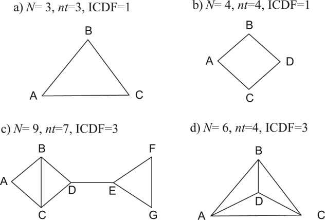
Possible treatment networks: treatments are represented by letters; lines connecting 2 treatments indicate that a comparison between these treatments has been made (in 1 or more randomized controlled trials).

$$\text{ICDF}=N-\left(nt-\text{1}\right).$$

This accords with the commonsense notion of inconsistency, which views it as a property of loops of evidence.^14,15 Every additional independent loop in a network of 2-arm trials represents 1 additional ICDF and one further way in which potential inconsistency can be realized.

In the square network in Figure 1b, there are N = 4 independent pieces of evidence, nt = 4 treatments, and nt − 1 = 3 parameters in a consistency model, giving ICDF = 4 − (4 − 1) = 1. In Figure 1c, there are N = 9 contrasts on which there is evidence, nt = 7 treatments, and 6 parameters, giving ICDF = 3. Note that the ICDF is equal to the number of independent loops. In Figure 1c, there are 2 separate structures in which inconsistency could be detected: the triangle EFG and the square ABCD. In the square, one could count a total of 3 loops: ABC, BCD, and ABCD. However, there are only 2 independent loops in this part of the structure: If we know all the edges of any 2 loops, we immediately know the edges of the third. Therefore, there can be only 2 inconsistencies in the ABCD square. Similarly, in Figure 1d, one can count a total of 7 loops: 4 three-treatment loops (ACD, BCD, ABD, ABC) and 3 four-treatment loops (ABCD, ACDB, CABD). But there are only 3 independent loops: N = 6, nt = 4, and ICDF = 3. It is not possible to specify which loops are independent, only how many there are because knowing the edges of any 3 loops will mean we know the edges of the others.

Multiarm Trials

When multiarm trials (i.e., trials with more than 2 arms) are included in the network, the definition of inconsistency becomes more complex. A 3-arm trial provides evidence on all 3 edges of an ABC triangle, and yet it cannot be inconsistent. In other words, although trial i estimates 3 parameters, δ_i,ΑΒ, δ_i,AC, δ_i,BC, only 2 are independent because δ_i,BC = δ_i,AC − δ_i,AB. There can therefore be no inconsistency within a 3-arm trial. Similarly, if all the evidence was from 3-arm trials on the same 3 treatments, there could be no inconsistency, only between-trials heterogeneity.

The difficulty in defining inconsistency comes when we have 2- and 3-arm trial evidence, for example, AB, AC, BC, and ABC trials. Because ICDF corresponds to the number of independent loops, if a loop is formed from a multiarm trial alone, it is not counted as an independent loop and must therefore be discounted from the total ICDF.⁶ Thus, where there are mixtures of 2-arm and multiarm trials, our definition of inconsistency as arising in loops creates inherent technical difficulties that cannot, as far as is known, be avoided.

Testing for Inconsistency

A key consideration in consistency assessment is whether independent tests for inconsistency can be constructed. These should be used wherever possible as they provide the simplest, most complete, and easiest to interpret analyses of inconsistency. We show how to construct independent tests, explain the circumstances where this is not possible, and set out methods for the more general case, which can be applied to any network.

Bucher Method for Single Loops of Evidence

The simplest method for testing consistency of evidence is essentially a 2-stage method.¹⁶ The first stage is to separately synthesize the evidence in each pairwise contrast; the second stage is to test whether direct and indirect evidence are in conflict. A direct estimate of the C versus B effect, ${\widehat{d}}_{BC}^{Dir}$, is compared with an indirect estimate, ${\widehat{d}}_{BC}^{Ind}$, formed from the AB and AC direct evidence

$${\widehat{d}}_{BC}^{Ind}={\widehat{d}}_{AC}^{Dir}-{\widehat{d}}_{AB}^{Dir}.$$ (1)

The direct estimates can be either from individual trials or from pairwise meta-analyses, whether fixed or random effects. Attached to each direct estimate is a variance, for example, ($\text{Var}({\widehat{d}}_{BC}^{Dir})$. As the direct estimates are statistically independent, we have $Var({\widehat{d}}_{BC}^{Ind})=Var({\widehat{d}}_{AC}^{Dir})+Var({\widehat{d}}_{AB}^{Dir})$ .

Estimates of the inconsistency, ω, and its variance can be formed by subtracting the direct and indirect estimates:

$$\begin{array}{l}{\widehat{\omega }}_{BC}={\widehat{d}}_{BC}^{Dir}-{\widehat{d}}_{BC}^{Ind}\\ \text{Var}({\widehat{\omega }}_{BC})=\text{Var}({\widehat{d}}_{BC}^{Dir})+\text{Var}({\widehat{d}}_{BC}^{Ind})\\ =\text{Var}({\widehat{d}}_{BC}^{Dir}\text{)}+\text{Var}({\widehat{d}}_{AB}^{Dir})+\text{Var}({\widehat{d}}_{AC}^{Dir}).\end{array}$$

An approximate test of the null hypothesis that there is no inconsistency is obtained by referring $z_{BC}=\frac{{\widehat{\omega }}_{BC}}{\sqrt{\text{Var}({\widehat{\omega }}_{BC})}}$ to the standard normal distribution.

It makes no difference whether we compare the direct BC evidence to the indirect evidence formed through AB and AC, or compare the direct AB evidence to the indirect AC and BC, or compare the AC with the AB and BC. The absolute values of the inconsistency estimates will be identical, as will the variances. This agrees with the intuition that, in a single loop, there can be only 1 inconsistency. However, this method can only be applied to 3 independent sources of data. Three-arm trials cannot be included because they are internally consistent and will reduce the chances of detecting inconsistency.

This method generalizes naturally to the square network in Figure 1b, which, like the triangle and any other simple circuit structure, has ICDF = 1. An indirect estimate of any edge can be formed from the remaining edges, and the variance of the inconsistency term is the sum of the variances of all the comparisons. For example, an indirect estimate ${\widehat{d}}_{BD}^{Ind}$ can be formed as ${\widehat{d}}_{BD}^{Ind}={\widehat{d}}_{AC}^{Dir}-{\widehat{d}}_{AB}^{Dir}+{\widehat{d}}_{CD}^{Dir}$, by successive application of the consistency equations. Clearly, as the number of edges in the loop increases, it becomes less and less likely that a real inconsistency will be detected because of the higher variance of the inconsistency estimate.

Extension to networks with multiple loops

Figure 1c represents a further pattern in which the inconsistency analysis can be broken down into separate independent elements: There are a total of 3 independent loops, and ICDF = 9 − (7 − 1) = 3. In this case, one inconsistency relates to the loop EFG, where there are 2 sources of evidence on any edge, whereas the other concerns the edge BC, on which there are 3 independent sources of evidence, 1 direct and 2 indirect. To analyze inconsistency in this structure, the problem is broken down into 2 separate and unrelated components. First, inconsistency in the EFG triangle is examined using the simple Bucher approach. Second, consistency between the 3 sources of evidence on the BC edge is examined by calculating a statistic to refer to a ${\chi }_2^2$ distribution.¹⁷ These 2 independent tests provide a complete analysis of the inconsistency in this network.

These methods are based on 2-arm trials. Inclusion of multiarm trials will lower their power to detect inconsistency. Our suggestion is that when a test on a loop ABC is being constructed, evidence from 3-arm ABC trials is excluded. However, ABC evidence on AB should be included when testing, for example, the ABD loop.

Methods for General Networks

Figure 1d shows a 4-treatment network in which there are data on every contrast and 3 possible inconsistencies. The difference between the networks in Figure 1d and Figure 1c is that in the former, there are 4 three-treatment loops (ACD, BCD, ABD, ABC) and 3 four-treatment loops (ABCD, ACDB, CABD), but these loops are not statistically independent. It is therefore not possible to construct a set of independent tests to examine the 3 inconsistencies.

Applying the Bucher method to each of the 7 loops in the network in turn would be a simple way to check inconsistency in this network. However, the number of loops, and hence the number of tests carried out, will far exceed the maximum number of possible inconsistencies in the network. For example, in a network where N = 42, nt = 12, and ICDF = 31,¹⁸ repeated use of the Bucher method on each of the 3-way loops in this network gave 70 estimates of inconsistency for the response outcome and 63 estimates for the acceptability outcome. In total, 6 loops showed statistically significant inconsistency, and the authors concluded that this was compatible with chance as 133 separate tests were performed. However, this could be questioned on the grounds that the 133 tests were not independent; there could not be more than 62 independent tests, and even this assumes that the 2 outcomes are unrelated.

Difficulties in the interpretation of statistical tests arise if any of the loops show significant inconsistency, at say a P < 0.05 level. One cannot immediately reject the null hypothesis at this level because multiple testing has taken place, and adjustment of significance levels would need to be considered. However, because the tests are not independent, calculating the correct level of adjustment becomes a complex task. Furthermore, in networks with multiple treatments, the total number of triangular, quadrilateral, and higher-order loops may be extremely large.

Unrelated mean effects model

In complex networks, where independent tests cannot be constructed, we propose that the standard consistency model^8,10 is compared with a model not assuming consistency. In the consistency model, a network with nt treatments, A, B, C, … defines nt − 1 basic parameters¹⁹ d_AB, d_AC, …, which estimate the effects of all treatments relative to treatment A, chosen as the reference treatment. Prior distributions are placed on these parameters. All other contrasts can be defined as functions of the basic parameters by making the consistency assumption.

We propose an unrelated mean effects (UME) model in which each of the N contrasts for which evidence is available represents a separate, unrelated, basic parameter to be estimated: no consistency is assumed. This model has also been termed inconsistency model.^9,20,21

Formally, suppose we have a set of M trials comparing nt = 4 treatments, A, B, C, and D, in any connected network. In an RE model, the study-specific treatment effects for a study comparing a treatment X to another treatment Y, δ_i,XY, are assumed to follow a normal distribution

$${\delta }_{i,XY}~N(d_{XY},{\sigma }^2)\text{for}i=1,\mathrm{\dots },M.$$ (2)

In a consistency model, nt − 1 = 3 basic parameters are given vague priors: d_AB, d_AC, d_AD ~N(0,100²), and the consistency equations define all other possible contrasts as

$$\begin{array}{l}{d}_{BC}=d_{AC}-d_{AB}\\ d_{BD}=d_{AD}-d_{AB}\\ d_{CD}=d_{AD}-d_{AC}.\end{array}$$ (3)

In an RE UME model, each of the mean treatment effects in equation 2 is treated as a separate (independent) parameter to be estimated, sharing a common variance σ². So, for the network in Figure 1d, the 6 treatment effects are all given vague priors: d_AB, d_AC, d_AD, d_BC, d_BD, d_CD ~ N(0,100²). Note that the extra number of parameters in this model is equal to the ICDF.

In an FE UME model, no shared variance parameter needs to be considered. The model is then equivalent to performing completely separate pairwise meta-analyses of the contrasts. However, fitting a UME model to all the data has the advantage of easily accommodating multiarm trials as well as providing a single global measure of model fit.

When multiarm trials are included in the evidence, the UME model can have different parameterizations depending on which of the multiple contrasts defined by a multiarm trial are chosen. For example, a 3-arm trial ABC can inform the AB and AC independent effects, or it can be chosen to inform the AB and BC effects (if B was the reference treatment), or the AC and BC effects (with C as reference). The code presented in the appendix arbitrarily chooses the contrasts relative to the first treatment in the trial. Thus, ABC trials inform the AB and AC contrasts, BCD trials inform BC and BD, and so forth. For FE models, the choice of parameterization makes no difference to the results, but in the RE model, the choice of parameterization will affect both the heterogeneity estimate and the tests of inconsistency.

Illustrative Examples

Smoking cessation

Twenty-four studies, including 2 three-arm trials, compared 4 smoking cessation counseling programs and recorded the number of individuals with successful smoking cessation at 6 to 12 mo.^3,6 All possible contrasts were compared, forming the network in Figure 1d, where A = no intervention, B = self-help, C = individual counseling, and D = group counseling.

We contrast a consistency model^8,10 with an RE model estimating 6 independent mean treatment effects. Results for both models are presented in Table 1, along with the posterior mean of the residual deviance and deviance information criterion (DIC), measures to assess model fit.²² Comparison between the deviance and DIC statistics of the consistency and UME models provides an omnibus test of consistency. In this case, the heterogeneity estimates, the posterior means of the residual deviance, and the DICs are very similar for both models.

Table 1.

Smoking Example: Posterior Summaries from Random Effects Consistency and Unrelated Mean Effects Models

	Network Meta-analysisa (Consistency Model)			Unrelated Mean Effects Model
	Mean/Median	SD	CrI	Mean/Median	SD	CrI
dAB	0.49	0.40	(−0.29, 1.31)	0.34	0.58	(−0.81, 1.50)
dAC	0.84	0.24	(0.39, 1.34)	0.86	0.27	(0.34, 1.43)
dAD	1.10	0.44	(0.26, 2.00)	1.43	0.88	(−0.21, 3.29)
dBC	0.35	0.41	(−0.46, 1.18)	−0.05	0.74	(−1.53, 1.42)
dBD	0.61	0.49	(−0.34, 1.59)	0.65	0.73	(−0.80, 2.12)
dCD	0.26	0.41	(−0.55, 1.09)	0.20	0.78	(−1.37, 1.73)
σ	0.82	0.19	(0.55, 1.27)	0.89	0.22	(0.58, 1.45)
resdevb	54.0			53.4
pD	45.0			46.1
DIC	99.0			99.5

Note: Mean, standard deviation (SD), 95% credible interval (CrI) of relative treatment effects, and median of between-trial standard deviation (σ) on the log-odds scale and posterior mean of the residual deviance (resdev), effective number of parameters (pD), and deviance information criterion. Results are based on 100 000 iterations on 3 chains after a burn-in period of 20 000 for the consistency model and after a burn-in of 30 000 for the inconsistency model. Treatments: A= no intervention, B = self-help, C = individual counseling, D = group counseling.

^a. d_BC, d_BD, d_CD calculated using the consistency equations.

^b.Compare to 50 data points.

Plotting the posterior mean deviance of the individual data points in the UME model against their posterior mean deviance in the consistency model (Figure 2) provides information that can help identify the loops in which inconsistency is present. We expect each data point to have a posterior mean deviance contribution of about 1, with higher contributions suggesting a poorly fitting model.²² In this example, the contributions to the deviance are very similar and close to 1 for both models. Two points have a higher than expected posterior mean deviance—these are the arms of 2 trials that have a zero cell—but the higher deviance is seen in both models. In general, trial arms with zero cells will have a high deviance as the model will never predict a zero cell exactly. The parameter estimates are similar for both models, and there is considerable overlap in the 95% credible intervals. This suggests no evidence of inconsistency in the network.

Figure 2.

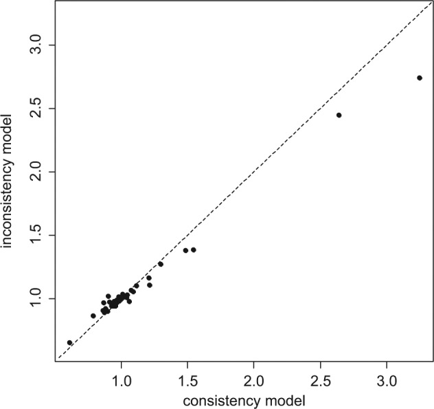
Plot of the individual data points’ posterior mean deviance contributions for the consistency model (horizontal axis) and the unrelated mean effects model (vertical axis) along with the line of equality.

Thrombolytic treatments

Figure 3 represents the treatment network for a data set consisting of 50 trials comparing 8 thrombolytic drugs and percutaneous transluminal coronary angioplasty, following acute myocardial infarction.^23,24 Data consist of the number of deaths in 30 or 35 days and the number of patients in each treatment arm. Note that in this network, not all treatment contrasts have been compared in a trial. There are 9 treatments in total and information on 16 pairwise comparisons, which would suggest an ICDF of 8. However, there is 1 loop, SK, Acc t-PA, SK+t-PA (highlighted in bold), which is only informed by a 3-arm trial and therefore cannot contribute to the number of possible inconsistencies. Discounting this loop gives ICDF = 7.²⁵

Figure 3.

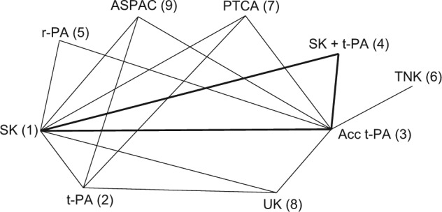
Thrombolytics example network. Lines connecting 2 treatments indicate that a comparison between these treatments (in 1 or more randomized controlled trials) has been made. The triangle highlighted in bold represents comparisons that have been made in only a 3-arm trial. Treatments: streptokinase (SK), alteplase (t-PA), accelerated alteplase (Acc t-PA), reteplase (r-PA), tenecteplase (TNK), urokinase (UK), anistreptilase (ASPAC), percutaneous transluminal coronary angioplasty (PTCA).

An FE NMA (consistency model) with a binomial likelihood and logit link^8,10 was fitted to the data, taking SK as the reference treatment, that is, the 8 treatment effects relative to SK are the basic parameters and have been estimated, whereas the remaining relative effects were obtained from the consistency assumptions. An FE model without the consistency assumptions was also fitted, which estimated 15 independent mean treatment effects (Table 2).

Table 2.

Thrombolitics Example: Posterior Summaries, Mean, Standard Deviation (SD), and 95% Credible Interval (CrI) on the Log-Odds Ratio Scale for Treatments Y versus X for Contrasts That Are Informed by Direct Evidence and Posterior Mean of the Residual Deviance (resdev), Number of Parameters (pD), and DIC for the Fixed Effects Network Meta-analysis and Inconsistency Models

Treatment		Network Meta-analysisa (Consistency Model)			Unrelated Mean Effects Model
X	Y	Mean	SD	CrI	Mean	SD	CrI
SK	t-PA	0.002	0.030	(−0.06, 0.06)	−0.004	0.030	(−0.06, 0.06)
SK	Acc t-PA	−0.177	0.043	(−0.26, −0.09)	−0.158	0.049	(−0.25, −0.06)
SK	SK + t-PA	−0.049	0.046	(−0.14, 0.04)	−0.044	0.047	(−0.14, 0.05)
SK	r-PA	−0.124	0.060	(−0.24, −0.01)	−0.060	0.089	(−0.23, 0.11)
SK	PTCA	−0.173	0.077	(−0.32, −0.02)	−0.665	0.185	(−1.03, −0.31)
SK	UK	−0.476	0.101	(−0.67, −0.28)	−0.369	0.518	(−1.41, 0.63)
SK	ASPAC	−0.203	0.221	(−0.64, 0.23)	0.005	0.037	(−0.07, 0.08)
t-PA	PTCA	0.016	0.037	(−0.06, 0.09)	−0.544	0.417	(−1.38, 0.25)
t-PA	UK	−0.180	0.052	(−0.28, −0.08)	−0.294	0.347	(−0.99, 0.37)
t-PA	ASPAC	−0.052	0.055	(−0.16, 0.06)	−0.290	0.361	(−1.01, 0.41)
Acc t-PA	r-PA	−0.126	0.067	(−0.26, 0.01)	0.019	0.066	(−0.11, 0.15)
Acc t-PA	TNK	−0.175	0.082	(−0.34, −0.01)	0.006	0.064	(−0.12, 0.13)
Acc t-PA	PTCA	−0.478	0.104	(−0.68, −0.27)	−0.216	0.119	(−0.45, 0.02)
Acc t-PA	UK	−0.206	0.221	(−0.64, 0.23)	0.146	0.358	(−0.54, 0.86)
Acc t-PA	ASPAC	0.013	0.037	(−0.06, 0.09)	1.405	0.417	(0.63, 2.27)
resdevb		105.9			99.7
pD		58			65
DIC		163.9			164.7

Note: Results are based on 50 000 iterations on 2 chains after a burn-in period of 50 000 for the consistency model and after a burn-in of 20 000 for the inconsistency model. Treatments: streptokinase (SK), alteplase (t-PA), accelerated alteplase (Acc t-PA), reteplase (r-PA), tenecteplase (TNK), urokinase (UK), anistreptilase (ASPAC), percutaneous transluminal coronary angioplasty (PTCA).

^a.All relative treatment effects not involving SK were calculated using the consistency equations.

^b.Compare to 102 data points.

Although the UME model is a better fit (lower posterior mean of the residual deviance), the DICs are very similar for both models because the UME model has 7 more parameters than the NMA model does. A plot of the individual data points’ posterior mean deviance contribution in each of the 2 models highlights 4 data points that fit poorly to the consistency model (Figure 4). These points correspond to the 2 arms of trials 44 and 45, which were the only 2 trials comparing Acc t-PA to ASPAC. Furthermore, the posterior estimates of the treatment effects of ASPAC versus Acc t-PA (Table 2) in the consistency and UME models differ markedly. The fact that the 2 trials on this contrast give similar results to each other but are in conflict with the remaining evidence supports the notion that there is a systematic inconsistency.

Figure 4.

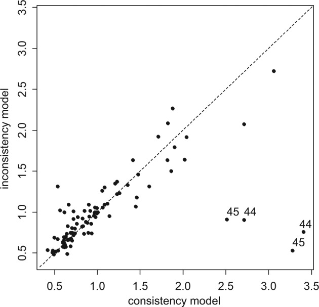
Plot of the individual data points’ posterior mean deviance contributions for the consistency model (horizontal axis) and the unrelated mean effects model (vertical axis) along with the line of equality. Points that have a better fit in the unrelated mean effects model have been marked with the trial number.

Other Methods for Detecting Inconsistency

Variance measures of inconsistency

In the UME models described above, a different basic parameter represents each contrast. One can reparameterize the 6-parameter UME model so that instead of 6 treatment effect parameters (d _AB, d _AC, d _AD, d _BC, d _BD, d _CD) we have (d _AB, d _AC, d _AD, ω_BC, ω_BD, ω_CD), where

$$\{\begin{array}{l}{\omega }_{BC}=d_{BC}-(d_{AC}-d_{AB})\\ {\omega }_{BD}=d_{BD}-(d_{AD}-d_{AB})\\ {\omega }_{CD}=d_{CD}-(d_{AD}-d_{AC})\end{array}.$$

The ω_BC, ω_BD, ω_CD parameters are the inconsistencies between the direct and indirect evidence on these 3 edges. However, rather than considering the 3 inconsistency parameters as unrelated, we might assume that they all come from a random distribution, for example, ω_XY, ~ N(0,${\sigma }_{\omega }^2$), where this additional between-contrast variance serves as a measure of inconsistency.^6,15 We do not recommend this, however, because measures of variance will have very wide credible intervals unless the ICDF is extremely high. Even then, large numbers of large trials on each contrast would be required to obtain a meaningful estimate. Furthermore, where there is a single loop (ICDF = 1), it should be impossible to obtain any estimate of ${\sigma }_{\omega }^2$. See Salanti and others²⁶ for further comments on this issue.

Node splitting

A more sophisticated approach, which needs to be implemented in a Bayesian MCMC framework, is node splitting.²⁵ This is a powerful and robust method that can be recommended as a further option for inconsistency analysis in complex networks. It allows the user to split the information contributing to estimates of a parameter (node), say, d _XY, into 2 distinct components: the direct based on all the XY data (which may come from XY, XYZ, WXY trials) and the indirect based on all the remaining evidence. The process can be applied to any contrast (node) in the network and in networks of any complexity. Like the UME model above, a shared variance term solves the difficulties created in an RE model when some contrasts are supported by only 1 or 2 trials. Node splitting can also generate intuitive graphics showing the difference between the estimates based on direct, indirect, and combined evidence.

Discussion

Although it is essential to carry out tests for inconsistency, this should not be considered in an overly mechanical way. Detection of inconsistency, like the detection of any statistical interaction, requires far more data than is needed to establish the presence of a treatment effect. The null hypothesis of consistency will therefore nearly always fail to be rejected, although this does not mean that there is no inconsistency.

The mechanisms that potentially could create bias in indirect comparisons appear be to identical to those that cause heterogeneity in pairwise meta-analysis. Thus, to ensure that conclusions based on indirect evidence are sound, we must attend to the direct evidence on which they are based, as is clear from equation 1. This states that if the direct estimates of the AB and AC effects are unbiased estimates of the treatment effects in the target population, the indirect estimate of the BC effect must be unbiased as well. Conversely, any bias in the direct estimates, for example, due to effect-modifying covariates arising from the patients not being drawn from the target population, will be passed on to the indirect estimates in equal measure. The term bias in this context must be seen broadly, comprising both internal and external threats to validity.²⁷ So if the direct evidence on AB is based on trials conducted on a patient population different from the target, and a treatment effect modifier is present, using the AB trials to draw inferences about the target population can be considered as (external) bias, which will be inherited by any indirect estimates based on these data.

Thus, the question, “Are conclusions based on indirect evidence reliable?” should be considered alongside the question, “Are conclusions based on pairwise meta-analysis reliable?” Any steps that can be taken to avoid between-trial heterogeneity will be effective in reducing the risk of drawing incorrect conclusions from pairwise meta-analysis, indirect comparisons, and NMA alike.

In the decision-making context, the most obvious sources of potential heterogeneity of effect, such as differences in dose or differences in cotherapies, will already have been eliminated when defining the scope, which is likely to restrict the set of trials to specific doses and cotherapies.

Clear cases in which direct and indirect evidence are in conflict are rare in the literature.^14,28 Where inconsistency has been evident, it illustrates the danger introduced by heterogeneity and in particular by the practice of trying to combine evidence on disparate treatment doses or treatment combinations within meta-analyses, often termed lumping.^1,29

The place for an enquiry into consistency is alongside a consideration of heterogeneity and its causes and, where appropriate, the reduction of heterogeneity through covariate adjustment (meta-regression) and bias adjustment.^27,30,31 This suggests that the risk of inconsistency is greatly reduced if between-trial heterogeneity is low. Empirical assessment of heterogeneity can therefore provide some reassurance or alert investigators to the risk of inconsistency. Tests of homogeneity in the pairwise comparisons can be used, or the posterior summaries of the distribution of the between-trials standard deviation can be compared to the size of the mean treatment effects. A second useful indicator is the between-trials variation in the trial baselines. If the treatment arms representing placebo or a standard treatment have similar proportions of events, this suggests that the trial populations are relatively homogeneous and that there will be little heterogeneity in the treatment effects. If, on the other hand, the baselines are highly heterogeneous, there is a potential risk of heterogeneity in the relative effects. Heterogeneity in baselines can be examined via a Bayesian synthesis.^32,33

One possible cause of inconsistency is a poor choice of scale of measurement, which can also lead to increased heterogeneity.^20,34 It is not always obvious whether to model treatment effects on a risk difference, logit, or other scale. The choice of the most appropriate scale is essentially an empirical one, although there is seldom enough evidence to decide on the basis of goodness of fit.^8,10

The choice of method used to test for inconsistency should be guided by the evidence structure. If it is possible to construct independent tests, then the Bucher method or its extensions represent the most simple and complete approach. In more complex networks, a repeated application of the Bucher method to all the possible loops produces interpretable results as long as no “significant” inconsistencies are found. Each application of the Bucher method is a valid test at its stated significance level. However, if inconsistencies are found when applying the test to all loops in the network, correction for multiple testing is needed, but it is difficult to specify how this should be done.

In networks where multiarm trials are included, assessment of inconsistency becomes more problematic, as the presence of such internally consistent trials tends to hide potential inconsistencies. Our suggestion of removing multiarm trials involved in the loop being checked can become quite cumbersome when there are multiple multiarm trials and multiple loops. Furthermore, removal of some trials may affect the estimated between-trials heterogeneity, which in turn may affect the detection of inconsistency. A careful examination of the network, paying special attention to which contrasts are informed by multiarm trials, how large these trials are, and how they are likely to affect estimates, is recommended. This can inform both the simple Bucher approach and the parameterization of the UME model.

Within a Bayesian framework, a consistency model can be compared with a model without the consistency assumptions. Analyses of residual deviance can provide an omnibus test of global inconsistency and can also help locate it. Node splitting²⁵ is another effective method for comparing direct evidence to indirect evidence in complex networks, but measures of inconsistency variance⁶ or incoherence variance¹⁵ are not recommended as indicators of inconsistency.

Although the Bucher approach is conceptually simpler and easy to apply, it requires 2 stages, whereas Bayesian approaches have the advantage of being one stage: There is no need to summarize the findings on each contrast first. The 2-stage approach introduces a particular difficulty in networks in which the evidence on some contrasts may be limited to a small number of trials. This is that the decision as to whether to fit an RE model must be taken for each contrast separately, and if there is only one study, only an FE analysis is available, even when there is clear evidence of heterogeneity on other contrasts. This causes a further problem: Under the null hypothesis of consistency that the method sets out to test, the true variances have to conform to special relationships known as “triangle inequalities,”⁹ but separate estimation makes it hard to ensure these inequalities are met. The likelihood of detecting an inconsistency, therefore, will be highly sensitive to the pattern of evidence. The choice of FE or RE summaries in the first stage can determine whether inconsistency is detected in the second stage.¹⁷ Interestingly, the UME model with its shared variance parameter offers a way of smoothing the estimates of between-trial heterogeneity.

Sparse data also show drawbacks in the Bayesian methods, especially when an RE analysis is used. The difficulty is that the greater the degree of between-trials heterogeneity, the less likely it is for inconsistency to be detectable, but there is seldom enough data to estimate the between-trials variation. The practice of using vague prior distributions for the between-trials variation, combined with a lack of data, will generate posteriors that allow an unrealistically high variance. This, in turn, is likely to mask all but the most obvious signs of inconsistency.

Although possible inconsistency should be investigated thoroughly, the preferred approach should be to consider potential sources of heterogeneity in advance.

Finally, there has been little work on how to respond to inconsistency when it is detected in a network. It is a reasonable principle that decisions should be based on models that are internally coherent, that is, models in which d _YZ = d _XZ − d _XY, and that these models should fit the data. If the data cannot be fitted by a coherent model, then some kind of adjustment must be made. Any adjustment in response to inconsistency is post hoc, and usually there will be a large number of different adjustments to the body of data that could eliminate the inconsistency. There are clear examples of this in the literature on multiparameter evidence synthesis in epidemiology applications,^35,36 emphasizing the importance of identifying potential causes of heterogeneity of effect at the scoping stage and potential internal biases in advance of synthesis. Similarly, although inconsistency in one part of the network does not necessarily imply that the entire body of evidence is to be considered suspect, a reexamination of all included studies is desirable.

Inconsistency is not a property of individual studies but of loops of evidence, and it may not always be possible to isolate which loop is responsible for the detected inconsistency, let alone which edge.⁶ Where several alternative adjustments are available, a sensitivity analysis is essential.

Appendix: WinBUGS Code for Illustrative Examples

Below, we set out code to fit random and fixed effects NMA and UME models to any network with a binomial likelihood and logit link function. In Dias and others,^8,10 a generalized linear model framework was introduced, with explanations of how the code for the binomial/logit model could be adapted for other likelihoods and link functions, including Poisson/log, Normal/identity, and other models. The models below can be adapted in exactly the same way.

The code below is fully general and will work for any number of multiarm trials with any number of arms. It is suitable for networks in which there is information on all possible treatment contrasts (such as in the smoking example presented in the article) or where there is information on just a subset of possible contrasts (such as in the thrombolytic treatments example in the article). However, in the latter case, the WinBUGS output from the UME model for contrasts that have no information will be redundant; that is, the posterior distribution will be equal to the prior, and no inferences can be made on these contrasts. We therefore recommend a careful consideration of the network structure before looking at the WinBUGS output from the UME code below.

Smoking Cessation: Network Meta-analysis RE Model, Binomial Likelihood

# Binomial likelihood, logit link

# Random effects model for multi-arm trials

model{        # *** PROGRAM STARTS

for(i in 1:ns){        # LOOP THROUGH STUDIES

w[i,1] <- 0         # adjustment for multi-arm trials is zero for control arm

delta[i,1] <- 0        # treatment effect is zero for control arm

mu[i] ~ dnorm(0,.0001)      # vague priors for all trial baselines

for (k in 1:na[i]) {        # LOOP THROUGH ARMS

r[i,k] ~ dbin(p[i,k],n[i,k])      # binomial likelihood

logit(p[i,k]) <- mu[i] + delta[i,k]      # model for linear predictor

rhat[i,k] <- p[i,k] * n[i,k]      # expected value of the numerators

dev[i,k] <- 2 * (r[i,k] * (log(r[i,k])-log(rhat[i,k])) #Deviance contribution

+ (n[i,k]-r[i,k]) * (log(n[i,k]-r[i,k]) - log(n[i,k]-rhat[i,k]))) }

resdev[i] <- sum(dev[i,1:na[i]])      # summed residual deviance contribution for this trial

for (k in 2:na[i]) {        # LOOP THROUGH ARMS

delta[i,k] ~ dnorm(md[i,k],taud[i,k])     # trial-specific LOR distributions

md[i,k] <- d[t[i,k]] - d[t[i,1]] + sw[i,k]     # mean of LOR distributions (with multi-arm trial correction)

taud[i,k] <- tau *2*(k-1)/k      # precision of LOR distributions (with multi-arm trial correction)

w[i,k] <- (delta[i,k] - d[t[i,k]] + d[t[i,1]])     # adjustment for multi-arm RCTs

sw[i,k] <- sum(w[i,1:k-1])/(k-1)      # cumulative adjustment for multi-arm trials

}

}

totresdev <- sum(resdev[])  # Total Residual Deviance

d[1]<-0     # treatment effect is zero for reference treatment

for (k in 2:nt){ d[k] ~ dnorm(0,.0001) }  # vague priors for treatment effects

sd ~ dunif(0,5)     # vague prior for between-trial SD

tau <- pow(sd,-2)     # between-trial precision = (1/between-trial variance)

# pairwise ORs and LORs for all possible pair-wise comparisons

for (c in 1:(nt-1)) {

for (k in (c+1):nt) {

or[c,k] <- exp(d[k] - d[c])

lor[c,k] <- (d[k]-d[c])

}

}

}    # *** PROGRAM ENDS

# Data (Smoking example)

# nt=no. treatments, ns=no. studies

list(nt=4,ns=24 )

r[,1] n[,1] r[,2] n[,2] r[,3] n[,3] t[,1] t[,2] t[,3] na[]

9 140 23 140 10 138 1 3 4 3 # trial 1 ACD

11 78 12 85 29 170 2 3 4 3 # trial 2 BCD

75 731 363 714 NA 1 1 3 NA 2 # 3

2 106 9 205 NA 1 1 3 NA 2 # 4

58 549 237 1561 NA 1 1 3 NA 2 # 5

0 33 9 48 NA 1 1 3 NA 2 # 6

3 100 31 98 NA 1 1 3 NA 2 # 7

1 31 26 95 NA 1 1 3 NA 2 # 8

6 39 17 77 NA 1 1 3 NA 2 # 9

79 702 77 694 NA 1 1 2 NA 2 # 10

18 671 21 535 NA 1 1 2 NA 2 # 11

64 642 107 761 NA 1 1 3 NA 2 # 12

5 62 8 90 NA 1 1 3 NA 2 # 13

20 234 34 237 NA 1 1 3 NA 2 # 14

0 20 9 20 NA 1 1 4 NA 2 # 15

8 116 19 149 NA 1 1 2 NA 2 # 16

95 1107 143 1031 NA 1 1 3 NA 2 # 17

15 187 36 504 NA 1 1 3 NA 2 # 18

78 584 73 675 NA 1 1 3 NA 2 # 19

69 1177 54 888 NA 1 1 3 NA 2 # 20

20 49 16 43 NA 1 2 3 NA 2 # 21

7 66 32 127 NA 1 2 4 NA 2 # 22

12 76 20 74 NA 1 3 4 NA 2 # 23

9 55 3 26 NA 1 3 4 NA 2 # 24

END

# Initial values

# Chain 1

list(sd=1, mu=c(0,0,0,0,0, 0,0,0,0,0, 0,0,0,0,0, 0,0,0,0,0, 0,0,0,0) )

# Chain 2

list(sd=1.5, mu=c(0,2,0,-1,0, 0,1,0,-1,0, 0,0,0,10,0, 0,10,0,0,0, 0,-2,0,0))

# Chain 3

list(sd=3, mu=c(0,0,0,0,0, 0,0,0,0,0, 0,0,0,0,0, 0,0,0,0,0, 0,0,0,0))

Smoking Cessation: UME RE Model, Binomial Likelihood

# Binomial likelihood, logit link, unrelated mean effects model

# Random effects model

model{            # *** PROGRAM STARTS

for(i in 1:ns){            # LOOP THROUGH STUDIES

delta[i,1]<-0            # treatment effect is zero in control arm

mu[i] ~ dnorm(0,.0001)            # vague priors for trial baselines

for (k in 1:na[i]) {            # LOOP THROUGH ARMS

r[i,k] ~ dbin(p[i,k],n[i,k])           # binomial likelihood

logit(p[i,k]) <- mu[i] + delta[i,k]           # model for linear predictor

rhat[i,k] <- p[i,k] * n[i,k]        # expected value of the numerators

dev[i,k] <- 2 * (r[i,k] * (log(r[i,k])-log(rhat[i,k]))     #Deviance contribution

+ (n[i,k]-r[i,k]) * (log(n[i,k]-r[i,k]) - log(n[i,k]-rhat[i,k])))

}

resdev[i] <- sum(dev[i,1:na[i]])           # summed residual deviance contribution for this trial

for (k in 2:na[i]) { # LOOP THROUGH ARMS

delta[i,k] ~ dnorm(d[t[i,1],t[i,k]] ,tau)       # trial-specific LOR distributions

}

}

totresdev <- sum(resdev[])           # Total Residual Deviance

for (c in 1:(nt-1)) {             # priors for all mean treatment effects

for (k in (c+1):nt) { d[c,k] ~ dnorm(0,.0001) }

}

sd ~ dunif(0,5)             # vague prior for between-trial standard deviation

var <- pow(sd,2)             # between-trial variance

tau <- 1/var             # between-trial precision

}              # *** PROGRAM ENDS

# Data is the same as for network meta-analysis model

#Initial values

# chain 1

list(sd=1, mu=c(0,0,0,0,0, 0,0,0,0,0, 0,0,0,0,0, 0,0,0,0,0, 0,0,0,0),

d = structure(.Data = c(NA,0,0,0, NA, NA,0,0, NA,NA,NA,0), .Dim = c(3,4)))

# chain 2

list(sd=1.5, mu=c(0,2,0,-1,0, 0,1,0,-1,0, 0,0,0,10,0, 0,10,0,0,0, 0,-2,0,0),

d = structure(.Data = c(NA,-2,0,5, NA, NA,0,2, NA,NA,NA,5), .Dim = c(3,4)))

# chain 3

list(sd=3, mu=c(0,0,0,0,0, 0,0,0,0,0, 0,0,0,0,0, 0,0,0,0,0, 0,0,0,0),

d = structure(.Data = c(NA,-3,-3,-3, NA, NA,-3,-3, NA,NA,NA,-3), .Dim = c(3,4)))

Thrombolytic Treatments: Network Meta-analysis FE Model, Binomial Likelihood

# Binomial likelihood, logit link

# Fixed effects model

model{      # *** PROGRAM STARTS

for(i in 1:ns){      # LOOP THROUGH STUDIES

mu[i] ~ dnorm(0,.0001)   # vague priors for all trial baselines

for (k in 1:na[i]) {    # LOOP THROUGH ARMS

r[i,k] ~ dbin(p[i,k],n[i,k])   # binomial likelihood

logit(p[i,k]) <- mu[i] + d[t[i,k]] - d[t[i,1]] # model for linear predictor

rhat[i,k] <- p[i,k] * n[i,k]   # expected value of the numerators

dev[i,k] <- 2 * (r[i,k] * (log(r[i,k])-log(rhat[i,k])) #Deviance contribution

+ (n[i,k]-r[i,k]) * (log(n[i,k]-r[i,k]) - log(n[i,k]-rhat[i,k])))

}

resdev[i] <- sum(dev[i,1:na[i]])   # summed residual deviance contribution for this trial

}

totresdev <- sum(resdev[])   # Total Residual Deviance

d[1]<-0      # treatment effect is zero for reference treatment

for (k in 2:nt){ d[k] ~ dnorm(0,.0001) } # vague priors for treatment effects

# pairwise ORs

for (c in 1:(nt-1)) {

for (k in (c+1):nt) {

or[c,k] <- exp(d[k] - d[c])

lor[c,k]<-(d[k]-d[c])

}

}

}   # *** PROGRAM ENDS

# Data (Thrombolytic treatments example)

#nt=no. treatments, ns=no. studies;

list(nt=9,ns=50)

r[,1] n[,1] r[,2] n[,2] r[,3] n[,3] t[,1] t[,2] t[,3] na[] # study ID

1472 20251 652 10396 723 10374 1 3 4 3 # 1

9 130 6 123 NA NA 1 2 NA 2 # 2

5 63 2 59 NA NA 1 2 NA 2 # 3

3 65 3 64 NA NA 1 2 NA 2 # 4

887 10396 929 10372 NA NA 1 2 NA 2 # 5

1455 13780 1418 13746 1448 13773 1 2 9 3 # 6

7 85 4 86 NA NA 1 2 NA 2 # 7

12 159 7 157 NA NA 1 2 NA 2 # 8

10 135 5 135 NA NA 1 2 NA 2 # 9

4 107 6 109 NA NA 1 4 NA 2 # 10

285 3004 270 3006 NA NA 1 5 NA 2 # 11

11 149 2 152 NA NA 1 7 NA 2 # 12

1 50 3 50 NA NA 1 7 NA 2 # 13

8 58 5 54 NA NA 1 7 NA 2 # 14

1 53 1 47 NA NA 1 7 NA 2 # 15

4 45 0 42 NA NA 1 7 NA 2 # 16

14 99 7 101 NA NA 1 7 NA 2 # 17

9 41 3 46 NA NA 1 7 NA 2 # 18

42 421 29 429 NA NA 1 7 NA 2 # 19

2 44 3 46 NA NA 2 7 NA 2 # 20

13 200 5 195 NA NA 2 7 NA 2 # 21

2 56 2 47 NA NA 2 7 NA 2 # 22

3 55 1 55 NA NA 3 7 NA 2 # 23

10 94 3 95 NA NA 3 7 NA 2 # 24

40 573 32 565 NA NA 3 7 NA 2 # 25

2 61 3 62 NA NA 3 7 NA 2 # 26

16 419 20 421 NA NA 3 7 NA 2 # 27

5 69 3 71 NA NA 3 7 NA 2 # 28

5 75 5 75 NA NA 3 7 NA 2 # 29

59 782 52 790 NA NA 3 7 NA 2 # 30

5 81 2 81 NA NA 3 7 NA 2 # 31

16 226 12 225 NA NA 3 7 NA 2 # 32

8 66 6 71 NA NA 3 7 NA 2 # 33

522 8488 523 8461 NA NA 3 6 NA 2 # 34

356 4921 757 10138 NA NA 3 5 NA 2 # 35

13 155 7 169 NA NA 3 5 NA 2 # 36

10 203 7 198 NA NA 1 8 NA 2 # 37

3 58 2 52 NA NA 1 9 NA 2 # 38

3 86 6 89 NA NA 1 9 NA 2 # 39

3 58 2 58 NA NA 1 9 NA 2 # 40

13 182 11 188 NA NA 1 9 NA 2 # 41

2 26 7 54 NA NA 3 8 NA 2 # 42

12 268 16 350 NA NA 3 8 NA 2 # 43

5 210 17 211 NA NA 3 9 NA 2 # 44

3 138 13 147 NA NA 3 9 NA 2 # 45

8 132 4 66 NA NA 2 8 NA 2 # 46

10 164 6 166 NA NA 2 8 NA 2 # 47

6 124 5 121 NA NA 2 8 NA 2 # 48

13 164 10 161 NA NA 2 9 NA 2 # 49

7 93 5 90 NA NA 2 9 NA 2 # 50

END

#Initial Values

#chain 1

list(d=c( NA, 0,0,0,0,0,0,0,0), mu=c(0,0,0,0,0, 0,0,0,0,0, 0,0,0,0,0, 0,0,0,0,0, 0,0,0,0,0, 0,0,0,0,0, 0,0,0,0,0, 0,0,0,0,0, 0,0,0,0,0, 0,0,0,0,0))

#chain 2

list(d=c( NA, -1,1,-1,1,1,-1,-2,2), mu=c(-3, -3, -3, -3, -3, -3, -3, -3, -3, -3, -3, -3, -3, -3, -3, -3, -3, -3, -3, -3, -3, -3, -3, -3, -3, -3, -3, -3, -3, -3, -3, -3, -3, -3, -3, -3, -3, -3, -3, -3, -3, -3, -3, -3, -3, -3, -3, -3, -3, -3))

#chain 3

list(d=c( NA, 2,-1,5,1,1,1,-1,-1), mu=c(-3, -3, -7, -3, -3, -3, -3, -3, -3, -3, -3, 1, 3,3, 3, -3, -3, -3, -3, -3, -3, 5, -3, -3, -3, -3, -3, -3, -5, -3, -3, -3, 5, -3, -3, -3, 8, -3, -3, -3, -3, 3, 3, 3, -3, -3, 3, -3, -3, 3))

Thrombolytic Treatments: UME FE Model, Binomial Likelihood

# Binomial likelihood, logit link, unrelated mean effects model

# Fixed effects model

model{      # *** PROGRAM STARTS

for(i in 1:ns){      # LOOP THROUGH STUDIES

mu[i] ~ dnorm(0,.0001)      # vague priors for trial baselines

for (k in 1:na[i]) {      # LOOP THROUGH ARMS

r[i,k] ~ dbin(p[i,k],n[i,k])     # binomial likelihood

logit(p[i,k]) <- mu[i] + d[t[i,1],t[i,k]]   # model for linear predictor

rhat[i,k] <- p[i,k] * n[i,k]     # expected value of the numerators

dev[i,k] <- 2 * (r[i,k] * (log(r[i,k])-log(rhat[i,k])) #Deviance contribution

+ (n[i,k]-r[i,k]) * (log(n[i,k]-r[i,k]) - log(n[i,k]-rhat[i,k])))

}

resdev[i] <- sum(dev[i,1:na[i]])    # summed residual deviance contribution for this trial

}

totresdev <- sum(resdev[])     # Total Residual Deviance

for (k in 1:nt) { d[k,k] <- 0 }     # set effects of k vs k to zero

for (c in 1:(nt-1)) {       # priors for all mean treatment effects

for (k in (c+1):nt) { d[c,k] ~ dnorm(0,.0001) }

}

}        # *** PROGRAM ENDS

# Data is the same as for network meta-analysis model

# Initial values

# chain 1

list(mu=c(0,0,0,0,0, 0,0,0,0,0, 0,0,0,0,0, 0,0,0,0,0, 0,0,0,0,0,

0,0,0,0,0, 0,0,0,0,0, 0,0,0,0,0, 0,0,0,0,0, 0,0,0,0,0),

d = structure(.Data = c(NA,0,0,0,0,0,0,0,0, NA,NA,0,0,0,0,0,0,0, NA,NA,NA,0,0,0,0,0,0, NA,NA,NA,NA,0,0,0,0,0, NA,NA,NA,NA,NA,0,0,0,0, NA,NA,NA,NA,NA,NA,0,0,0, NA,NA,NA,NA,NA,NA,NA,0,0, NA,NA,NA,NA,NA,NA,NA,NA,0, NA,NA,NA,NA,NA,NA,NA,NA,NA), .Dim = c(9,9)) )

# chain 2

list(mu=c(0,0,10,0,-1, 0,0,0,0,0, 0,0,0,0,0, 0,0,0,0,0, 0,0,0,0,0,

0,0,0,0,0, 3,0,0,-2,0, 0,0,-1,0,0, 0,-0.5,5,0.5,0.5, 0,0,0,2,0),

d = structure(.Data = c(NA,0,1,0,0,-2,0,0,0, NA,NA,0,0,2,0,0,-2,0, NA,NA,NA,0,0,0,0,0,0, NA,NA,NA,NA,0,0,0,0,0, NA,NA,NA,NA,NA,0,0,1,0, NA,NA,NA,NA,NA,NA,0,0,-2, NA,NA,NA,NA,NA,NA,NA,0,0, NA,NA,NA,NA,NA,NA,NA,NA,0, NA,NA,NA,NA,NA,NA,NA,NA,NA), .Dim = c(9,9)) )

# chain 3

list(mu=c(0,0,10,0,5, 0,0,0,0,0, 0,0,0,0,0, 0,0,0,0,0, 0,0,0,0,0,

0,0,0,0,0, 3,0,0,-2,0, 0,0,-8,0,0, 0,-0.5,5,0.5,0.5, 0,0,0,2,0),

d = structure(.Data = c(NA,0,1,0,0,-5,0,5,0, NA,NA,0,0,3,0,0,-2,0, NA,NA,NA,0,0,0,0,0,0, NA,NA,NA,NA,0,0,0,0,0, NA,NA,NA,NA,NA,0,-5,1,0, NA,NA,NA,NA,NA,NA,0,0,-4, NA,NA,NA,NA,NA,NA,NA,0,0, NA,NA,NA,NA,NA,NA,NA,NA,0, NA,NA,NA,NA,NA,NA,NA,NA,NA), .Dim = c(9,9)) )

References

- 1. Caldwell DM, Ades AE, Higgins JPT. Simultaneous comparison of multiple treatments: combining direct and indirect evidence. BMJ. 2005;331:897–900 [DOI] [PMC free article] [PubMed] [Google Scholar]
- 2. Gleser LJ, Olkin I. Stochastically dependent effect sizes. In: Cooper H, Hedges LV, eds. The Handbook of Research Synthesis. New York: Russell Sage Foundation; 1994. p 339–55 [Google Scholar]
- 3. Hasselblad V. Meta-analysis of multi-treatment studies. Med Decis Making. 1998;18:37–43 [DOI] [PubMed] [Google Scholar]
- 4. Higgins JPT, Whitehead A. Borrowing strength from external trials in a meta-analysis. Stat Med. 1996;15:2733–49 [DOI] [PubMed] [Google Scholar]
- 5. Lu G, Ades A. Combination of direct and indirect evidence in mixed treatment comparisons. Stat Med. 2004;23:3105–24 [DOI] [PubMed] [Google Scholar]
- 6. Lu G, Ades A. Assessing evidence consistency in mixed treatment comparisons. J Am Stat Assoc. 2006;101:447–59 [Google Scholar]
- 7. Glenny AM, Altman DG, Song F, et al. Indirect comparisons of competing interventions. Health Technol Assess. 2005;9(26):1–134 [DOI] [PubMed] [Google Scholar]
- 8. Dias S, Welton NJ, Sutton AJ, Ades AE. NICE DSU Technical Support Document 2: A Generalised Linear Modelling Framework for Pair-wise and Network Meta-analysis. NICE Decision Support Unit; 2011. Available from: URL: http://www.nicedsu.org.uk [PubMed]
- 9. Lu G, Ades AE. Modelling between-trial variance structure in mixed treatment comparisons. Biostatistics. 2009;10:792–805 [DOI] [PubMed] [Google Scholar]
- 10. Dias S, Sutton AJ, Ades AE, Welton NJ. Evidence synthesis for decision making 2: a generalized linear modeling framework for pairwise and network meta-analysis of randomized controlled trials. Med Decis Making. 2013;33(5):607-617 [DOI] [PMC free article] [PubMed] [Google Scholar]
- 11. Song F, Loke Y-K, Walsh T, Glenny A-M, Eastwood AJ, Altman DG. Methodological problems in the use of indirect comparisons for evaluating healthcare interventions: survey of published systematic reviews. BMJ. 2009;338(31):b1147. [DOI] [PMC free article] [PubMed] [Google Scholar]
- 12. Cranney A, Guyatt G, Griffith L, et al. Summary of meta-analyses of therapies for post-menopausal osteoporosis. Endocr Rev. 2002;23(4):570–8 [DOI] [PubMed] [Google Scholar]
- 13. Lunn DJ, Thomas A, Best N, Spiegelhalter D. WinBUGS—a Bayesian modelling framework: concepts, structure, and extensibility. Stat Comput. 2000;10:325–37 [Google Scholar]
- 14. Song F, Altman D, Glenny A-M, Deeks J. Validity of indirect comparison for estimating efficacy of competing interventions: evidence from published meta-analyses. BMJ. 2003;326:472–6 [DOI] [PMC free article] [PubMed] [Google Scholar]
- 15. Lumley T. Network meta-analysis for indirect treatment comparisons. Stat Med. 2002;21:2313–24 [DOI] [PubMed] [Google Scholar]
- 16. Bucher HC, Guyatt GH, Griffith LE, Walter SD. The results of direct and indirect treatment comparisons in meta-analysis of randomized controlled trials. J Clin Epidemiol. 1997;50(6):683–91 [DOI] [PubMed] [Google Scholar]
- 17. Caldwell DM, Welton NJ, Ades AE. Mixed treatment comparison analysis provides internally coherent treatment effect estimates based on overviews of reviews and can reveal inconsistency. J Clin Epidemiol. 2010;63:875–82 [DOI] [PubMed] [Google Scholar]
- 18. Cipriani A, Furukawa TA, Salanti G, et al. Comparative efficacy and acceptability of 12 new generation antidepressants: a multiple-treatments meta-analysis. Lancet. 2009;373:746–58 [DOI] [PubMed] [Google Scholar]
- 19. Eddy DM, Hasselblad V, Shachter R. Meta-analysis by the Confidence Profile Method. London: Academic Press; 1992 [Google Scholar]
- 20. Caldwell DM, Welton NJ, Dias S, Ades AE. Selecting the best scale for measuring treatment effect in a network meta-analysis: a case study in childhood nocturnal enuresis. Res Synth Meth. 2012;3:126–141 [DOI] [PubMed] [Google Scholar]
- 21. Dias S, Welton NJ, Sutton AJ, Caldwell DM, Lu G, Ades AE. NICE DSU Technical Support Document 4: Inconsistency in Networks of Evidence Based on Randomised Controlled Trials. NICE Decision Support Unit; 2011. Available from: URL: http://www.nicedsu.org.uk [PubMed]
- 22. Spiegelhalter DJ, Best NG, Carlin BP, van der Linde A. Bayesian measures of model complexity and fit. J R Stat Soc B. 2002;64(4):583–616 [Google Scholar]
- 23. Boland A, Dundar Y, Bagust A, et al. Early thrombolysis for the treatment of acute myocardial infarction: a systematic review and economic evaluation. Health Technol Assess. 2003;7(15):1–136 [DOI] [PubMed] [Google Scholar]
- 24. Keeley EC, Boura JA, Grines CL. Primary angioplasty versus intravenous thrombolytic therapy for acute myocardial infarction: a quantitative review of 23 randomised trials. Lancet. 2003;361:13–20 [DOI] [PubMed] [Google Scholar]
- 25. Dias S, Welton NJ, Caldwell DM, Ades AE. Checking consistency in mixed treatment comparison meta-analysis. Stat Med. 2010;29:932–44 [DOI] [PubMed] [Google Scholar]
- 26. Salanti G, Higgins JPT, Ades AE, Ioannidis JPA. Evaluation of networks of randomised trials. Stat Methods Med Res. 2008;17(3):279–301 [DOI] [PubMed] [Google Scholar]
- 27. Turner RM, Spiegelhalter DJ, Smith GCS, Thompson SG. Bias modelling in evidence synthesis. J R Stat Soc A. 2009;172:21–47 [DOI] [PMC free article] [PubMed] [Google Scholar]
- 28. Song F, Xiong T, Parekh-Bhurke S, et al. Inconsistency between direct and indirect comparisons of competing interventions: meta-epidemiological study. BMJ. 2011;343:d4909. [DOI] [PMC free article] [PubMed] [Google Scholar]
- 29. Caldwell DM, Gibb DM, Ades AE. Validity of indirect comparisons in meta-analysis. Lancet. 2007;369(9558):270. [DOI] [PubMed] [Google Scholar]
- 30. Dias S, Sutton AJ, Welton NJ, Ades AE. Evidence synthesis for decision making 3: heterogeneity–subgroups, meta-regression, bias, and bias-adjustment. Med Decis Making. 2013;33(5):618-640 [DOI] [PMC free article] [PubMed] [Google Scholar]
- 31. Dias S, Welton NJ, Marinho VCC, Salanti G, Higgins JPT, Ades AE. Estimation and adjustment of bias in randomised evidence by using mixed treatment comparison meta-analysis. J R Stat Soc A. 2010;173(3):613–29 [Google Scholar]
- 32. Dias S, Welton NJ, Sutton AJ, Ades AE. NICE DSU Technical Support Document 5: Contructing the Baseline Model. NICE Decision Support Unit; 2011. Available from: URL: http://www.nicedsu.org.uk
- 33. Dias S, Welton NJ, Sutton AJ, Ades AE. Evidence synthesis for decision making 5: the baseline natural history model. Med Decis Making. 2013;33(5):657-670 [DOI] [PMC free article] [PubMed] [Google Scholar]
- 34. Deeks JJ. Issues on the selection of a summary statistic for meta-analysis of clinical trials with binary outcomes. Stat Med. 2002;21:1575–600 [DOI] [PubMed] [Google Scholar]
- 35. Goubar A, Ades AE, De Angelis D, et al. Estimates of human immunodeficiency virus prevalence and proportion diagnosed based on Bayesian multiparameter synthesis of surveillance data. J R Stat Soc A. 2008;171:541–80 [Google Scholar]
- 36. Presanis A, De Angelis D, Spiegelhalter D, Seaman S, Goubar A, Ades A. Conflicting evidence in a Bayesian synthesis of surveillance data to estimate HIV prevalence. J R Stat Soc A. 2008;171:915–37 [Google Scholar]