Voxelwise quantification of [¹¹C](R)-rolipram PET data: a comparison between model-based and data-driven methods

Abstract

This study compared model-based and data-driven methods to assess the best methodology for generating precise and accurate parametric maps of the parameters of interest in [¹¹C](R)-rolipram brain positron-emission tomography studies. Parametric images were generated using (1) a two-tissue compartmental model (2TCM) solved with the hierarchical basis function method (H-BFM) linear estimator; (2) data-driven spectral-based methods: standard spectral analysis (std SA) and rank-shaping SA (RS); and (3) the Logan graphical plot. Nonphysiologic V_T estimates were eliminated and the remaining ones were compared with the reference values, i.e., those obtained with a voxelwise 2TCM solved with a nonlinear estimator. With regard to voxelwise V_T estimates, H-BFM showed the best agreement with weighted nonlinear least square (WNLLS) values and the lowest percentage of mean relative difference (1±1%). All methods showed comparable variability in the relative differences. H-BFM provided the best correlation with WNLLS (y=1.034x−0.013; R²=0.973). Despite a slight bias, the other three methods also showed good agreement and high correlation (R²>0.96). H-BFM yielded the most reliable voxelwise quantification of [¹¹C](R)-rolipram as well as the complete description of the tracer kinetic. The Logan plot represents a valid alternative if only V_T estimation is required. Its marginally higher bias was outweighed by a low computational time, ease of implementation, and robustness.

Introduction

[¹¹C](R)-rolipram is a positron-emission tomography radioligand for the quantification in vivo of phosphodiesterase type IV, an enzyme that metabolizes 3′,5′-cyclic adenosine monophosphate. The cyclic adenosine monophosphate cascade plays an important role in major depressive disorder (MDD) and is a potential target for drug development. In particular, postmortem brain studies found that multiple markers of the cyclic adenosine monophosphate cascade were decreased in patients with MDD.^{1, 2, 3, 4} Rodent experiments have similarly shown that chronic administration of antidepressants upregulates several components of the cyclic adenosine monophosphate cascade, including phosphodiesterase type IV.⁵ A recently published study using PET and [¹¹C](R)-rolipram showed for the first time that phosphodiesterase type IV is downregulated in vivo in unmedicated individuals with MDD.⁶

As phosphodiesterase type IV is ubiquitously distributed in the brain, no appropriate reference regions exist that are devoid of specific binding. Consequently, noninvasive reference tissue models, such as the simplified reference tissue model⁷ or the multilinear reference tissue model,⁸ cannot be used for [¹¹C](R)-rolipram quantification, and the acquisition of an arterial input function for kinetic modeling is unavoidable.

A previous study in humans showed that the pharmacokinetics of [¹¹C](R)-rolipram is well described by a two-tissue four-rate constant compartmental model (2TCM), and that Logan graphical analysis yielded similar results at the region of interest (ROI) level.⁹ While the Logan plot allows the easy computation of parametric images for the total distribution volume (V_T), it does not account for the vascular component within the voxel, and generally underestimates the parameter of interest in noisy data,¹⁰ especially when applied voxelwise. Nevertheless, the resulting bias is almost constant and thus, these limitations can be neglected when using the Logan plot in statistical comparison between different groups of subjects.

It is important to note, however, that voxelwise analysis of the whole kinetic of the tracer in tissues may yield the ability to generate quantitatively accurate parametric maps and thus harness the full potential of [¹¹C](R)-rolipram for the study of MDD and related diseases. Towards this end, different strategies, based on compartmental modeling or data-driven approaches, may be used to generate parametric maps.

In general, model-driven methods require the definition of the compartmental structure that best describes the behavior of the tracer, with specific assumptions about the number of compartments and their connections. The present study applied the 2TCM proposed in the literature at the ROI level⁹ at the voxel level, and solved it with a nonlinear estimator. Nonlinear estimators typically have significant drawbacks when applied to voxelwise estimation (i.e., sensitivity to initial estimates, high computational time, nonconvergence in a significant percentage of voxels). To overcome these problems, we performed 2TCM analysis in conjunction with the hierarchical-basis function method (H-BFM), as implemented by Rizzo et al.¹¹ This method uses a linear estimator to identify the parameters of the classic compartmental model at the voxel level, and integrates information derived at the ROI level.

In contrast, data-driven methods require no a priori definition of the model structure, because this information is derived directly from the kinetic data. Furthermore, data-driven methods generally require less restrictive initial hypotheses compared with model-driven methods. The present study used standard spectral analysis (std SA), as developed by Cunningham and Jones,¹² and the rank-shaping regularization of the std SA (RS), developed by Turkheimer et al.¹³ In SA, the kinetic activity of the tracer in the tissue is described by the sum of decaying exponentials convolved with an input function, and the coefficients of a predefined set of biologically plausible exponential basis functions are estimated using non-negative least squares to fit the data. This technique also provides information about the number of compartments necessary to describe the data. The SE allows investigators to characterize the transfer function of the system even if the actual relationship of these parameters to the physiologic measures is possible only with prior knowledge of the biochemical properties of the tracer and the model structure. Based on the same hypothesis as std SA, RS implements a filtering procedure optimized for quantification of reversible tracers without using the non-negativity constraints of the least squares estimator of SA. Therefore, RS is less sensitive to the noise associated with voxelwise images and might improve the calculation of parametric maps.

This study aimed to assess the best methodology for voxelwise quantification of [¹¹C](R)-rolipram in brain PET studies to generate precise and accurate parametric maps of the parameters of interest.

MATERIALS AND METHODS

Radioligand Preparation

[¹¹C](R)-rolipram was synthesized as previously described¹⁴ and, according to the Investigational New Drug Application #73,149, submitted to the US Food and Drug Administration. A copy of the application is available at: http://pdsp.med.unc.edu/snidd/nidpulldownPC.php. The radioligand was obtained in high radiochemical purity (>99%).

Image Acquisition

Data obtained from 10 healthy subjects enrolled in a previous study⁶ were used. The protocol was approved by the Ethics Committee of the National Institutes of Health; all subjects gave written informed consent.

All PET images were acquired using an Advance tomograph (GE Medical Systems, Waukesha, WI, USA) after a bolus injection of 695±152 MBq (range, 727 to 756) of [¹¹C](R)-rolipram, with the exception of one subject who had 264 MBq. An 8-minute ⁶⁸Ge transmission scan was obtained before injection of the radiotracer for attenuation correction. Dynamic image data were acquired in 3D mode for 90 minutes, which is adequate to measure the V_T of [¹¹C](R)-rolipram with small bias and good identifiability.⁹ The dynamic scan comprised 27 frames (6 × 30, then 3 × 60, 2 × 120, and 16 × 300 seconds). Positron-emission tomography data were reconstructed on a 128 × 128 matrix with a pixel size of 2.0 × 2.2 × 4.25 mm³. For scanning protocol and image reconstruction details, the interested reader is referred to Fujita et al.⁶

During the acquisition, blood samples (1 ml each) were drawn from the radial artery at 15-second intervals until 150 seconds, followed by 3-ml samples at 3, 4, 6, 8, 10, 15, 20, 30, 40, and 50 minutes, and 4.5 ml at 60, 75, and 90 minutes. Decay-corrected whole-blood activity, the fraction of unchanged radioligand in plasma, and the plasma/whole blood ratio were calculated as described previously.^{14, 15}

Each subject also underwent a high-resolution 3D T1-weighted magnetic resonance imaging (MRI) scan using either a 3-T Signa scanner (GE Medical Systems) or an Achieva 3-T MRI scanner (Philips Health Care, Andover, MA, USA). The MRI data sets were used to derive the anatomic information necessary to define ROIs.

Compartmental Model

The model proposed in the literature for use in both animals and humans to describe [¹¹C](R)-rolipram kinetics in brain tissue is a 2TCM.^{9, 14} The model includes an arterial plasma component (C_p) and two-tissue compartments, one describing the nondisplaceable component (C_nd) and one describing the specific binding (C_s), as follows:

where the microparameters K₁ (ml/cm³ per minute), k₂ (min⁻¹), k₃ (min⁻¹), and k₄ (min⁻¹) are the rate constants for tracer transport from plasma to tissue and back, and from the nondisplaceable compartment to the specific one and back, respectively. Thus, the concentration of radioactivity in tissue at time t (C_T) can be expressed as

Once the concentration of [¹¹C](R)-rolipram in tissues has been defined, the measurement equation (C_meas) that also takes into account the contribution of tracer in blood in a specified volume of observation is given by

where C_b represents the concentration of the tracer in the whole blood, including radiometabolites (kBq/ml), and V_b is the fraction of blood volume, which is unitless.

Knowledge of the system microparameters also makes it possible to derive V_T (ml/cm³), which is defined as the ratio of the tracer concentration in the tissue to the metabolite-corrected plasma concentration at equilibrium. In the case of the 2TCM model, V_T can be calculated as

To quantify [¹¹C](R)-rolipram with a 2TCM at the voxel level, we selected a set of approaches based on the reversibility of tracer kinetics already described in the literature (detailed below). In particular, we chose those methods appropriate to the analysis of tracers with reversible kinetics, robust to the low signal-to-noise ratio of the voxel time–activity curves (TACs), and that are optimized to estimate the volume of distribution parametric maps.

Compartmental modeling solved with a nonlinear estimator

The 2TCM microparameters (k₁, k₂, k₃, k₄, and V_b) were quantified for each voxel TAC by using the WNLLS, as implemented in Matlab2011b (The Mathworks, Natick, MA, USA) by the lsqnonlin.m function. This approach was used based on the assumption that the model that describes tracer kinetics in the ROI can also be extended at the voxel level. For each subject, the initial parameters were derived from the 2TCM applied at the ROI level. The convergence criteria were set as defaults as implemented in Matlab. We set no upper bounds and lower bounds were set equal to zero. Although 2TCM has been reported as the model of choice for describing the kinetic of [¹¹C](R)-rolipram,⁹ in the present study we also generated parametric images with a 1TCM solved with a nonlinear estimator.

We assessed the performance of both models for fitting ROI TACs using the Akaike Information Criterion, the visual comparison of the data model fit, the precision of the estimates expressed as their between-subject s.d., and the percentage of model failures at the voxel level.

Compartmental modeling solved with a linear estimator: hierarchical basis function method

Because of the weakness of the nonlinear estimator applied at the voxel level (convergence issues, high computational time, sensitivity to initial estimates), we also identified the 2TCM using H-BFM, as implemented by Rizzo et al.¹¹ H-BFM identifies all the system micro- and macroparameters (i.e., k₁, k₂, k₃, k₄, V_b, V_T and nondisplaceable binding potential (BP_ND)) following a hierarchical scheme from ROI to voxel analysis. In fact, the results obtained by solving the 2TCM for each ROI TAC (segmented using anatomic information) with WNLLS were used a priori to automatically generate local grids for voxel-by-voxel analysis. From the regionwise estimates, one two-dimensional grid was evaluated for each ROI and set to be 20 × 20 elements. From the grids, a set of basis functions consisting of exponential terms convolved with the input function were defined, and the model was then solved with a linear estimator, choosing as the best solution the one that minimized the weighted residual sum of squares. To derive this method, the interested reader is referred to the original reference by Rizzo et al.¹¹

Data-Driven Spectral-Based Methods

Standard spectral analysis

Spectral analysis is based on a time-invariant single input/single output model, used to identify the kinetic components of tissue tracer activity, without fixing a priori the number of compartments in the system.¹² In SA, the concentration of radioactivity in tissue at time t, C_T(t), is modeled as a convolution of the plasma time–activity curve, C_p(t), with the sum of M+1 distinct exponential terms given as

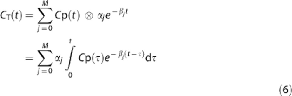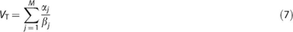
where α_j and β_j are assumed to be real valued and non-negative. Not all compartmental models satisfy these assumptions, but they are met by the kinetic models used with many PET tracers,¹⁶ including [¹¹C](R)-rolipram. In equation (6) the maximum number of terms to be included in the model, M+1, is predefined and set to an arbitrary large number, e.g., 100. Possible values of β_j are fixed to cover a biologic plausible spectral range, and values of α_j are estimated from blood and tissue TACs by a non-negative linear least squares procedure, as implemented in Matlab by the lsqnonneg.m function. In practice, only a few components with α_j>0 are detected.¹⁷ The factors determining which components are identified are the definition of the grid, the measurement error affecting the data, the sensitivity of the radioactivity to the changes in the intervals of the exponents, the algorithm chosen, and the convergence criteria.¹⁸ It must be recalled that the components of the spectra do not depend on a specific model, and the interpretation of the parameters of the different components can be derived only on the basis of a structural model. However, from the estimated parameters, it is possible to derive the total binding rate constant (K_i, ml/cm³ per minute) for irreversible tracers, or the total volume of distribution (V_T ),¹⁸ as in the case of [¹¹C](R)-rolipram. In particular, V_T was calculated from the estimated spectrum as

From the analysis of the kinetic spectrum, it is always possible to derive the tracer delivery from plasma to tissue (K₁) as the sum of α_j estimated amplitudes. Moreover, it is possible to derive blood volume information (V_b) by combining the measurement equation (equation (4)) with the SA tissue kinetic model (equation (6)). The grids for the β_j's of equation (6) were defined as a logarithmic distribution of β_j, j=1, 2, …, M,^{18, 19} with M set equal to 100. The lower and upper limits of the distribution were defined as β₁=1/(3T_end) and β_M=(3/T_in), where T_end and T_in, respectively, represent the end time of the scan (T_end=90 min) and the duration of the first scan (T_in=0.25 minutes). The spacing of the β_j's was thus fixed as

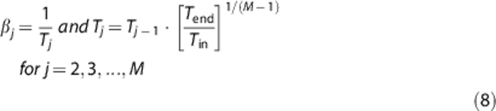This distribution guarantees that all the possible kinetics measurable within the specific time window of the experiment and its sampling times can be detected with SA.¹² The M unknown values α_j were estimated with the weighted non-negative linear least squares algorithm implemented in Matlab.

Rank-shaping spectral analysis

To overcome the high sensitivity of the std SA to the noise in the voxel data, we also applied an improved variation of the RS SA method.¹³ Rank shaping is a Bayesian development of std SA, optimized for reversible tracers, which works on the same principles as SA but does not rely on the non-negativity constraints of non-negative least squares. It implements a Kalman filter of the estimated kinetic spectrum to provide reliable estimates of V_T, which is the only outcome measure for this method. For the derivation of RS, the interested reader is referred to the original reference by Turkheimer et al.¹³

The grids were defined as described above for the std SA. However, RS also required the signal-to-noise ratio interval bound values to be set, representing the signal-to-noise ratio expected in the tissue data. Commonly, 1/signal-to-noise ratio has been fixed at 1% as shown in the original paper.¹³ However, different settings (5%, 20%) did not significantly change the results.

Graphical Logan Analysis

In addition to the methods described above, we also quantified [¹¹C](R)-rolipram binding with Logan analysis.²⁰ Logan plot is a model-independent graphical method and allows the parameters of interest to be estimated quickly. It transforms the data so that, after a certain time (t>t*), the data show a linear trend whose slope can be related to the V_T, according to

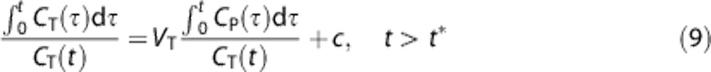It must be noted that Logan analysis neither accounts for the blood volume nor allows the full description of the whole time course of the tracer in the tissues. Moreover, it has been shown to be highly sensitive to noise in the data, resulting in a bias in the final results, especially when applied voxelwise.¹⁰

For Logan analysis, the optimal value of the equilibrium point t* of equation (9) was chosen by visual inspection of several Logan plots and set to use the last 12 frames for the estimation. We checked the impact of using different number of frames for the Logan analysis, and the relative differences on the estimated parameters were less than 1%.

Error Measurements

All the quantification methods were implemented with relative weighted estimators. Weights were derived as the inverse of the variance of the PET measurement error, which was assumed to be additive and uncorrelated from a Gaussian distribution with zero mean. Its covariance matrix was defined from the noise error count less than a scale factor γ. The proportionality constant γ was estimated a posteriori as in Bertoldo et al..²¹

Data Preprocessing

Brain ROI segmentation

A probabilistic atlas was generated in standard stereotaxic space (MNI/ICBM152) by merging the Harvard–Oxford cortical, subcortical, and cerebellum structural atlases made available via FMRIB Software Library.^{22, 23} We considered right and left hemispheres combined for a total of 48 cortical and 10 subcortical regions.

To coregister the atlas to the individual subject's MR, the MR image of the Montreal Neurologic Institute brain template was normalized to each subject's MR image by applying a linear registration as implemented in FSL (FMRIB Software Library),^{24, 25} and the atlas was registered to the subject's MR space by applying the normalization parameters. The rigid transformation for MRI-to-PET coregistration was derived in the same way from FSL linear registration and applied to the original MRI and the transformed maximum probability atlas, resulting in all the images being coregistered with the unchanged PET image data set. Finally, we multiplied the atlas in PET space and derived the 58 ROI TACs, obtained by averaging the voxel TACs belonging to each of the 58 anatomic regions. The MR and the PET image summed across the whole time scan along with the coregistered MR and anatomic atlas of a representative subject are given in Figure 1.

Figure 1.

Brain images of one representative subject. (A) Magnetic resonance imaging (MRI) T1 weighted in its original space. (B) Summed dynamic [¹¹C](R)-rolipram PET image over time. (C) Anatomic atlas co-registered in PET space. For each panel, figures are reported in axial and sagittal views.

Arterial modeling

For all subjects, the measured input function values (C_p(t), kBq/ml) were preprocessed before the quantification using both the measured samples and the fit of the plasma data to the three-exponential model proposed by Feng et al.²⁶ The mathematical expression for Feng's plasmatic model without the delay factor is given by

where λ₁, λ₂, and λ₃ (in min⁻¹) are the eigenvalues of the model and A₁ (in kBq/ml/min), A₂, and A₃ (in kBq/ml) represent the coefficients of the model. The delay values were provided from previous analysis.⁹ The model was solved by minimizing the weighted residual sum of squares. Weights were defined as the inverse of the variance associated to the arterial measures, which was modeled assuming Poisson statistics. Feng's model provided a reliable description of the washout (from peak to tail), but made it difficult to properly describe the impulsive shape of the arterial time curves;²⁶ thus, we constrained the model at the peak of the arterial measurements (t_peak) to the maximum of the arterial samples (C_peak), as follows:

Based on the visual analysis of the model fit and the comparison of the weighted residuals, Feng's model was chosen because it provided the best trade-off between data description and goodness of fit in this population of 10 subjects. However, choosing a different input function would not alter the results of this study, because all parametric maps for each subject were generated using the same input function.

Statistical Analysis

Results obtained at voxel level using 2TCM model solved with WNLLS were used as the reference values. From the parametric maps obtained with the different methods, we discarded those voxels with biologically implausible results, specifically those with V_T values ⩽0 and also those with V_T values >1.5 ml/cm³. This cutoff value was chosen because it is more than 100% higher than the maximum value found in the literature at the ROI level, i.e., V_T=0.73 ml/cm³ (ref. 9) and was not a conservative threshold, as doubling the upper bound did not affect the results (maximum difference⩽1%). The coefficient of variation (CV) was also considered to assess the precision of the different approaches, and it was calculated using the rule of error propagation. In addition, we also discarded QUOTE values with a CV higher than 50% or with an imaginary CV to eliminate unreliable estimates. In this case, we decided to maintain a conservative cutoff, in order to keep only reliable values. For each subject, we therefore only considered the subset of voxels in which all the methods reached convergence, and used the statistical analysis in these groups of voxels.

For each method, we averaged the V_T estimates obtained in the voxels composing each ROI, and considered only the subset of voxels in which all the methods converged. These average values were compared with the average of the V_T estimates obtained with WNLLS in the same voxels in terms of mean relative differences (m.r.d.'s).

The percentage m.r.d. (m.r.d.%) was calculated between the estimates obtained with WNLLS and the other methods (below indicated as met1 and met2):

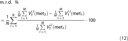where N is the number of subjects, M the number of voxels of the ROI, the value of WNLLS estimate in the lth voxel for the ith subject and the value of the other method's (std SA or RS or Logan or H-BFM) estimate in the lth voxel for the ith subject.

As the averaged results in the ROIs did not provide any information about variability within the system, we also evaluated the distribution of the relative differences of the voxel estimates between the alternative methods and the reference method, considering only those voxels that yielded both physiologic and reliable estimates. This analysis allowed the assessment of the voxelwise error variability and was performed in a subset of brain ROIs: hippocampus, amygdala, cerebellum, thalamus, frontal cortex, caudate, putamen, pallidum, and brain stem.⁹

Finally, we evaluated the correlation between the results with a regression analysis: the slope and the intercept of the fitted regression line with the mean of V_T WNLLS in each ROI as an independent variable and the mean of values obtained with the alternative methods in each ROI as dependent variable were calculated considering every ROI for all subjects. Pearson R² values were reported as a correlation measure.

Results

In line with previously reported results,⁹ 2TCM was a better model than 1TCM for describing [¹¹C](R)-rolipram data for most of the cerebral voxels and in all subjects (data not shown). For example, for the subject considered in Figure 1, 2TCM was the better model for 81% of the voxels; in the remaining voxels, it is likely that the high noise in the voxel TACs prevented the distinction of the two different kinetic components in the data, and the simpler model was selected as best. Therefore, 1TCM was not used for any subsequent analyses.

All the parametric maps are presented before correction for the outliers in Figure 2 for the same representative subject shown in Figure 1. Here, both WNLLS and SA V_T estimates were visually very noisy, while H-BFM, RS, and Logan had only a limited or negligible amount of outlying voxels (Table 1). The weighted nonlinear least square yielded the poorest image quality, and more than 50% of the voxels had to be eliminated (Table 1). In particular, 16% on average of the voxels had to be discarded for nonphysiologic estimates, 29% for values with a CV ⩾50%, and 12% for values with an imaginary CV. Moreover, WNLLS required high computational time (up to five times greater than the other methods). Although the V_T estimates in the remaining voxels are considered as the reference values, these results clearly highlight the necessity of an alternative method for voxelwise quantification.

Figure 2.

Distribution volume (V_T) parametric maps obtained with (A) Weighted nonlinear least squares (WNLLS) applied to a two-tissue compartmental model, (B) standard spectral analysis (std SA), (C) Rank-shaping spectral analysis (RS), (D) Hierarchical Basis Function Method (H-BFM) and (E) Logan graphical analysis. Results refer to a transaxial slice at the cortical level for a representative subject. For this particular subject, the percentage of voxels outside the physiologic range (as defined in the Methods section) was less than 2% for SA (spectral analysis) (due to high V_T results) and 4% for H-BFM (due to the presence of some negative V_T values), but was as high as 24% for WNLLS.

Table 1. Analysis of outliers and failures: inter-subject variability.

	WNLLS	H-BFM	Logan	std SA	RS
Negative VT estimatesa
Mean	0.0%	6.2%	<0.001%	0.0%	0.0%
s.d.	0.0%	3.7%	<0.001%	0.0%	0.0%
Min	0.0%	1.0%	<0.001%	0.0%	0.0%
Max	0.0%	12.4%	<0.001%	0.0%	0.0%
Not physiologic VT estimates VTb
Mean	16.0%	0.3%	<0.001%	0.8%	<0.001%
s.d.	7.3%	0.9%	<0.001%	0.7%	<0.001%
Min	7.7%	<0.001%	<0.001%	<0.001%	<0.001%
Max	31.4%	2.8%	<0.001%	2.3%	<0.001%
Convergence problems (imaginary CV for VT)c
Mean	11.7%	<0.001%	<0.001%	<0.001%	<0.001%
s.d.	5.0%	<0.001%	<0.001%	<0.001%	<0.001%
Min	5.9%	<0.001%	<0.001%	<0.001%	<0.001%
Max	18.7%	<0.001%	<0.001%	<0.001%	<0.001%
Unreliable VT estimates 𝒞𝒱VTℰ𝒩𝒯ℐ𝒯𝒴𝒮𝒯𝒜ℛ𝒯ℰ𝒩𝒯ℐ𝒯𝒴ℰ𝒩𝒟d
Mean	28.5%	0.1%	<0.001%	3.9%	<0.001%
s.d.	9.5%	0.1%	<0.001%	1.3%	<0.001%
Min	15.2%	<0.001%	<0.001%	1.8%	<0.001%
Max	44.1%	0.2%	<0.001%	6.6%	<0.001%
Total number of outliers
Mean	56.2%	6.7%	<0.001%	4.7%	<0.001%
s.d.	5.4%	1.5%	<0.001%	0.7%	<0.001%

Abbreviations: CV, coefficient of variation; H-BFM, hierarchical basis function method; Logan, Logan graphical analysis; RS, rank-shaping spectral analysis; std SA, standard spectral analysis; s.d., standard deviation; V_T, distribution volume; WNLLS, weighted nonlinear least squares.

^aIntersubject variability of the fraction of voxel-negative V_T estimates with respect to the whole brain.

^bIntersubject variability of the fraction of not physiologic voxel V_T estimates with respect to the whole brain.

^cIntersubject variability of the fraction of voxels with estimator convergence issues with respect to the whole brain.

^dIntersubject variability of the fraction of unreliable voxel V_T estimates with respect to the whole brain.

When considering the mean values of V_T voxel estimates averaged within the subset of the different brain regions for all subjects, we found that H-BFM showed the smallest m.r.d. (1±1%) as compared with the reference of voxel WNLLS analysis. All other methods showed slightly more biased but comparable results in all the regions and all the subjects, along with a comparable variability in the relative differences (Table 2, Figure 3). Rank shaping showed a negative bias of ∼5%, probably because of the filtering procedure inherent to the method, which tends to remove high-frequency kinetic components along with noise. The Logan method performed the worst, with a m.r.d. of −6±2%.

Table 2. Correlation with the reference method (WNLLS).

	H-BFM	Logan	std SA	RS
Mean comparison: relative difference
Mean	1%	−6%	−4%	−5%
s.d.	1%	2%	1%	2%
Min	−1%	−12%	−6%	−11%
Max	5%	−2%	−2%	−1%
Linear regression
Slope	1.034	0.938	0.950	0.927
Intercept	−0.013	−0.001	0.006	0.013
R2	0.973	0.977	0.984	0.960

Abbreviations: H-BFM, hierarchical basis function method; Logan, Logan graphical analysis; RS, rank-shaping spectral analysis; std SA, standard spectral analysis; s.d., standard deviation; WNLLS, weighted nonlinear least squares.

Figure 3.

(A) Mean and variability of voxel V_T estimates within regions. Black, white, light-gray, gray, and dark-gray bars refer respectively to weighted nonlinear least squares (WNLLS), Hierarchical Basis Function Method (H-BFM), Logan analysis, standard spectral analysis (std SA), and Rank-shaping spectral analysis (RS). Results are computed considering all the 10 subjects in the study for some representative regions. (B) Mean relative differences (m.r.d.) of regional V_T estimates with respect to the reference (WNLLS). In order, from top to bottom, results are reported for H-BFM, Logan analysis, std SA, and RS. Dotted lines represent the mean of the m.r.d. between regions.

In terms of distribution of the voxel's relative differences of V_T, H-BFM showed the smallest m.r.d. across the cerebral volume (0.8±8.7%). Rank shaping yielded similar results, but with a slightly higher variability (−0.5±9.7%). Spectral analysis had the highest variability (−1±17%), while Logan results showed the most substantial V_T underestimation (−4±8.7%) (Figure 4). All differences were calculated in the intersection of brain voxels, where all methods lead to physiologic and reliable estimates.

Figure 4.

Distributions of m.r.ds. for voxel V_T estimates in a representative subject. Results are reported for Hierarchical Basis Function Method (H-BFM), standard spectral analysis (std SA), rank-shaping spectral analysis (RS) and Logan plot (panels A–D respectively) in comparison with the reference quantification method (weighted nonlinear least squares (WNLLS)). For each method, distribution mean and standard deviation are also reported.

All the methods yielded good agreement and high correlation with the reference values, as shown by the regression lines and Pearson's coefficient values (R²>0.96) (Figure 5 and Table 2). H-BFM agreed best with the WNLLS voxel estimates and had one of the highest correlations (R²=0.97), despite an average 6% of voxels yielding a negative V_T. Although the Logan plot most underestimated the parameter of interest, it was well correlated with reference values (R²=0.98). Despite a poorer image quality, std SA performed better than RS in terms of agreement and correlation (std SA: R²=0.98; RS: R²=0.96).

Figure 5.

Scatter plots of V_T estimates. The mean of V_T voxel parameter estimates within regions estimated using weighted nonlinear least squares (WNLLS) analysis (x axis) versus the mean of V_T voxel parameter estimates within regions estimated using (A) Hierarchical Basis Function Method (H-BFM), (B) Logan, (C) standard spectral analysis (std SA), and (D) rank-shaping spectral analysis (RS) (y axis) are reported for all subjects. In each scatter plot, the values of slope and intercept of the fitted regression line and Pearson's value R² are reported.

In terms of computational time, the fastest method was the Logan analysis (<5 minutes for an entire brain volume), followed by the spectral-based methods (∼2 hours each for both) and H-BFM (5–6 hours). As expected, the slowest method was WNLLS, with an average time of 20±3 hours (mean±s.d.) for a single subject analysis. Figure 1 of Supplementary material provides an example of the different model fits for two representative voxels, one belonging to the thalamus and one to the occipital cortex. For both voxels, no differences were observed in the model fits for 2TCM, H-BFM, or std SA. Only RS sometimes presented a different fit, but in general, it was always characterized by a higher residual sum of squares.

Discussion

Previous studies identified 2TCM as the optimal model to describe [¹¹C](R)-rolipram kinetics at the ROI level.⁹ The present work investigated whether this model could be extended to the voxel level, and confirmed that for the majority of the cerebral voxels 2TCM is a better model than 1TCM to describe [¹¹C](R)-rolipram binding. In the remaining voxels, it is likely that the high noise in the voxel TACs prevented the distinction of the two different kinetic components in the data, and therefore a simpler model (i.e., 1TCM) gave a better fit. In support of this hypothesis, no spatial clusterization of these voxels was found; instead, they were randomly spread across the cerebral volume. In terms of performance, however, voxelwise 2TCM solved with WNLLS was associated with high computational time (∼20 hours), poor image quality, and high percentage of outliers, underscoring the need for an alternative method of quantification at the voxel level.

When applied voxelwise, a 2TCM solved with WNLLS has significant disadvantages, such as sensitivity to initial estimates, high computational time, and nonconvergence in a significant percentage of voxels. These disadvantages could have been minimized by using two-compartmental fitting with constraints (e.g., fixing K₁/k₂ or k₄ to the values obtained from data at the regional level). This would have reduced computational time and improved image quality by reducing the number of outlying voxels. However, a constrained compartmental model, even if it improves identifiability, may theoretically introduce a bias in the results. Therefore, we chose an unconstrained fitting and selected those subsets of voxels whose V_T estimates showed physiologic values and good identifiability, and used them as the reference values. This choice was justified by the fact that when the nonlinear estimator was applied at the voxel level, the results obtained when it converged were characterized by the same properties as the estimator itself, i.e., nonpolarization, consistency, asymptotic normality, and efficiency.²⁷

Comparing alternative methodologies to 2TCM showed that (1) H-BFM was the method showing the smallest m.r.d. and one of the highest correlation, with a considerably smaller computational cost; (2) std SA provided useful information about tissue kinetics and blood volume and had a very small absolute quantification bias, but was associated with the highest variability of voxel estimates; (3) rank shaping gave results comparable to std SA in terms of absolute quantification, but had a significantly better image quality; (4) the Logan analysis was the fastest and simplest method but yielded the highest bias, though it was still comparable to those obtained with more technically demanding methods (e.g., RS); (5) notably, the results of the subject who received a lower injection activity (264 MBq) were comparable to those of the subjects who had a high injection activity (727 to 756 MBq). This suggests that the methods performance is robust with respect to the injection activity. Taken together, these results show that all the alternative approaches gave comparable results with the reference method (R² ⩾0.96 and absolute value of m.r.d.⩾6%); some of them improved map quality, or differed in their computational time and failure rate. Nevertheless, each method was associated with its own strengths and drawbacks, as elaborated below.

H-BFM provided the best estimates in terms of quantification compared with the reference method, and kept the computational time within reasonable limits (∼6 hours). Because it may be considered as a compartmental model optimized for voxelwise analysis, it allows the estimation of k₁, k₂, k₃, k₄, and V_b for each element of the PET image. In addition to having more detailed information about the physiology of the system under study, for tracers where the reference region is not available (such as [¹¹C](R)-rolipram), knowledge of the microparameters allows the calculation of other macroparameters in addition to V_T. For example, it is possible to obtain the BP_ND from the ratio of k₃ to k₄ or the nondisplaceable volume of distribution (V_ND) from the ratio of K₁ to k₂. In Supplementary material, Figures 2A and 2B report the BP_ND and V_ND, respectively, obtained with H-BFM for a representative subject. The results are in agreement with those previously reported inZanotti-Fregonara et al.⁹ Figures 2C and 2D report the K₁ and V_b parametric maps obtained with H-BFM providing extra information about the analyzed system of interest. In particular, the nonhomogenous spatial distribution of V_b estimates indicates the necessity of taking into account the blood fraction when analyzing [¹¹C](R)-rolipram data also at the voxel level.

However, the computational time was still more demanding than that associated with spectral approaches (up to three times as long as an RS analysis). It also had a higher failure rate than spectral-based approaches (in up to 8% of voxels).

Spectral analysis parametric maps were noisy compared with other methods, though they showed the highest correlation with reference values in the subset of voxels where all the methods converged. Despite having one of the smallest absolute values of m.r.d. (4%), std SA yielded the highest variability of voxel estimates (17%). However, it provided useful information about tissue kinetics and blood volume, which would be impossible to obtain with graphical approaches such as the Logan plot. It should be noted that the information derived by std SA about the number and type of components necessary to describe the [¹¹C](R)-rolipram kinetic at voxel level agreed with the 2TCM (data not shown).

Despite being an extension and improvement of std SA, RS provided comparable results in terms of agreement with the reference method. However, RS resulted in significantly better image quality with respect to std SA, with very few outlying voxels (<0.001%).

Logan analysis provided no insight regarding tracer kinetic behavior and blood volume estimation. Moreover, it was associated with a slightly higher bias than the other techniques. Nevertheless, the Logan plot was the simplest and fastest technique, and therefore well suited for clinical studies. Indeed, voxelwise Logan analysis has been successfully used to demonstrate a widespread reduction of [¹¹C](R)-rolipram binding in MDD patients compared with healthy controls.⁶ Moreover, the Logan plot is the only technique among those evaluated in the present study that potentially allows investigators to use a less invasive input function, such as an image-derived input function (IDIF) or a population-based input function (PBIF).²⁸ In fact, the Logan plot is relatively insensitive to errors in the shape of the input function as long as the total area under the curve is well estimated.²⁹ In contrast, model-driven and spectral-based approaches require that the shape of the input function, including the peak, be perfectly estimated. If the shape is wrong—a common event with both image-derived input function and population-based input function —then not only the microparameters but also the macroparameters, which are derived from the mathematical combination of the microparameters, will be erroneously estimated. The macroparameter V_T would be estimated reliably only if the errors of the microparameters cancel out and the integral of the input is preserved.

The present study did not consider variations on the Logan plot, such as the likelihood estimation graphical analysis,³⁰ the empirical Bayesian estimation in graphical analysis³¹ or the multilinear analysis³² because these methods do not provide any additional information compared with the Logan plot. Moreover, likelihood estimation graphical analysis and empirical Bayesian estimation in graphical analysis require the use of a nonlinear estimator, with all the associated convergence issues and computational heaviness.

Finally, the present study used [¹¹C](R)-rolipram as an example; nevertheless, the advantages and drawbacks described here for the different methods should not be particularly tracer-specific. Similar results are thus to be expected for any tracer with comparable kinetics in receptor binding studies.

Conclusion

In conclusion, different techniques exist to generate parametric images, and each has its own advantages and drawbacks. H-BFM allows a complete and reliable quantification of the [¹¹C](R)-rolipram kinetic at the voxel level. If the whole description of the tracer kinetics is not necessary, or if only the V_T estimate is required to compare different populations or in longitudinal studies, then the Logan plot represents a valid alternative. Its marginally higher bias is outweighed by the ease of implementation and robustness of the method.

The authors declare no conflict of interest.

References

- Cowburn RF, Marcusson JO, Eriksson A, Wiehager B, Oneill C. Adenylyl-cyclase activity and g-protein subunit levels in postmortem frontal-cortex of suicide victims. Brain Res. 1994;633:297–304. doi: 10.1016/0006-8993(94)91552-0. [DOI] [PubMed] [Google Scholar]
- Dwivedi Y, Conley RR, Roberts RC, Tamminga CA, Pandey GN. [3H]cAMP binding sites and protein kinase a activity in the prefrontal cortex of suicide victims. Am J Psychiatry. 2002;159:66–73. doi: 10.1176/appi.ajp.159.1.66. [DOI] [PubMed] [Google Scholar]
- Reiach JS, Li PP, Warsh JJ, Kish SJ, Young LT. Reduced adenylyl cyclase immunolabeling and activity in postmortem temporal cortex of depressed suicide victims. J Affect Disord. 1999;56:141–151. doi: 10.1016/s0165-0327(99)00048-8. [DOI] [PubMed] [Google Scholar]
- Dowlatshahi D, MacQueen GM, Wang JF, Young LT. Increased temporal cortex CREB concentrations and antidepressant treatment in major depression. Lancet. 1998;352:1754–1755. doi: 10.1016/S0140-6736(05)79827-5. [DOI] [PubMed] [Google Scholar]
- Duman RS, Malberg J, Thome J. Neural plasticity to stress and antidepressant treatment. Biol Psychiatry. 1999;46:1181–1191. doi: 10.1016/s0006-3223(99)00177-8. [DOI] [PubMed] [Google Scholar]
- Fujita M, Hines CS, Zoghbi SS, Mallinger AG, Dickstein LP, Liow JS, et al. Downregulation of brain phosphodiesterase type IV measured with 11C-(R)-rolipram PET in major depressive disorder. Biol Psychiatry. 2012;72:548–554. doi: 10.1016/j.biopsych.2012.04.030. [DOI] [PMC free article] [PubMed] [Google Scholar]
- Lammertsma AA, Hume SP. Simplified reference tissue model for PET receptor studies. Neuroimage. 1996;4:153–158. doi: 10.1006/nimg.1996.0066. [DOI] [PubMed] [Google Scholar]
- Ichise M, Liow JS, Lu JQ, Takano A, Model K, Toyama H, et al. Linearized reference tissue parametric imaging methods: application to [11C]DASB positron-emission tomography studies of the serotonin transporter in human brain. J Cereb Blood Flow Metab. 2003;23:1096–1112. doi: 10.1097/01.WCB.0000085441.37552.CA. [DOI] [PubMed] [Google Scholar]
- Zanotti-Fregonara P, Zoghbi SS, Liow JS, Luong E, Boellaard R, Gladding RL, et al. Kinetic analysis in human brain of [11C](R)-rolipram, a positron emission tomographic radioligand to image phosphodiesterase 4: a retest study and use of an image-derived input function. Neuroimage. 2011;54:1903–1909. doi: 10.1016/j.neuroimage.2010.10.064. [DOI] [PMC free article] [PubMed] [Google Scholar]
- Slifstein M, Laruelle M. Effects of statistical noise on graphic analysis of PET neuroreceptor studies. J Nucl Med. 2000;41:2083–2088. [PubMed] [Google Scholar]
- Rizzo G, Turkheimer FE, Bertoldo A. Multi-scale hierarchical approach for parametric mapping: assessment on multi-compartmental models. Neuroimage. 2013;67:344–353. doi: 10.1016/j.neuroimage.2012.11.045. [DOI] [PubMed] [Google Scholar]
- Cunningham VJ, Jones T. Spectral analysis of dynamic pet studies. J Cereb Blood Flow Metab. 1993;13:15–23. doi: 10.1038/jcbfm.1993.5. [DOI] [PubMed] [Google Scholar]
- Turkheimer FE, Hinz R, Gunn RN, Aston JAD, Gunn SR, Cunningham VJ. Rank-shaping regularization of exponential spectral analysis for application to functional parametric mapping. Phys Med Biol. 2003;48:3819–3841. doi: 10.1088/0031-9155/48/23/002. [DOI] [PubMed] [Google Scholar]
- Fujita M, Zoghbi SS, Crescenzo MS, Hong J, Musachio JL, Lu J-Q, et al. Quantification of brain phosphodiesterase 4 in rat with (R)-[11C]rolipram-PET. NeuroImage. 2005;26:1201–1210. doi: 10.1016/j.neuroimage.2005.03.017. [DOI] [PubMed] [Google Scholar]
- Zoghbi SS, Shetty HU, Ichise M, Fujita M, Imaizumi M, Liow JS, et al. PET imaging of the dopamine transporter with 18F-FECNT: a polar radiometabolite confounds brain radioligand measurements. J Nucl Med. 2006;47:520–527. [PubMed] [Google Scholar]
- Schmidt K. Which linear compartmental systems can be analyzed by spectral analysis of PET output data summed over all compartments. J Cereb Blood Flow Metab. 1999;19:560–569. doi: 10.1097/00004647-199905000-00010. [DOI] [PubMed] [Google Scholar]
- Press HW, Flannery BP, Teukolsky SA, Vetterling WT. Numerical Recipes: The Art of Scientific Computing. Cambridge University Press; 1986. [Google Scholar]
- Turkheimer F, Moresco RM, Lucignani G, Sokoloff L, Fazio F, Schmidt K. The use of spectral analysis to determine regional cerebral glucose utilization with positron-emission tomography and [f-18] fluorodeoxyglucose — theory, implementation, and optimization procedures. J Cereb Blood Flow Metab. 1994;14:406–422. doi: 10.1038/jcbfm.1994.52. [DOI] [PubMed] [Google Scholar]
- Distefano JJ. Optimized blood-sampling protocols and sequential design of kinetic-experiments. Am J Physiol. 1981;240:R259–R265. doi: 10.1152/ajpregu.1981.240.5.R259. [DOI] [PubMed] [Google Scholar]
- Logan J, Fowler JS, Volkow ND, Wolf AP, Dewey SL, Schlyer DJ, et al. Graphical analysis of reversible radioligand binding from time-activity measurements applied to [N-11C-methyl]-(−)cocaine PET studies in human subjects. J Cereb Blood Flow Metab. 1990;10:740–747. doi: 10.1038/jcbfm.1990.127. [DOI] [PubMed] [Google Scholar]
- Bertoldo A, Vicini P, Sambuceti G, Lammertsma AA, Parodi O, Cobelli C. Evaluation of compartmental and spectral analysis models of [F-18]FDG kinetics for heart and brain studies with PET. Ieee T Bio-Med Eng. 1998;45:1429–1448. doi: 10.1109/10.730437. [DOI] [PubMed] [Google Scholar]
- Smith SM, Jenkinson M, Woolrich MW, Beckmann CF, Behrens TEJ, Johansen-Berg H, et al. Advances in functional and structural MR image analysis and implementation as FSL. Neuroimage. 2004;23:S208–S219. doi: 10.1016/j.neuroimage.2004.07.051. [DOI] [PubMed] [Google Scholar]
- Woolrich MW, Jbabdi S, Patenaude B, Chappell M, Makni S, Behrens T, et al. Bayesian analysis of neuroimaging data in FSL. Neuroimage. 2009;45:S173–S186. doi: 10.1016/j.neuroimage.2008.10.055. [DOI] [PubMed] [Google Scholar]
- Jenkinson M, Bannister P, Brady M, Smith S. Improved optimization for the robust and accurate linear registration and motion correction of brain images. Neuroimage. 2002;17:825–841. doi: 10.1016/s1053-8119(02)91132-8. [DOI] [PubMed] [Google Scholar]
- Jenkinson M, Smith S. A global optimisation method for robust affine registration of brain images. Med Image Anal. 2001;5:143–156. doi: 10.1016/s1361-8415(01)00036-6. [DOI] [PubMed] [Google Scholar]
- Feng D, Huang SC, Wang XM. Models for computer-simulation studies of input functions for tracer kinetic modeling with positron-emission tomography. Int J Biomed Comput. 1993;32:95–110. doi: 10.1016/0020-7101(93)90049-c. [DOI] [PubMed] [Google Scholar]
- Cobelli C, Carson R. Introduction to Modeling in Physiology and Medicine. Elsevier/Academic Press: San Diego; 2001. [Google Scholar]
- Zanotti-Fregonara P, Hines CS, Zoghbi SS, Liow JS, Zhang Y, Pike VW, et al. Population-based input function and image-derived input function for [11C](R)-rolipram PET imaging: Methodology, validation, and application to the study of major depressive disorder. Neuroimage. 2012;63:1532–1541. doi: 10.1016/j.neuroimage.2012.08.007. [DOI] [PMC free article] [PubMed] [Google Scholar]
- Zanotti-Fregonara P, Chen K, Liow JS, Fujita M, Innis RB. Image-derived input function for brain PET studies: many challenges and few opportunities. J Cereb Blood Flow Metab. 2011;31:1986–1998. doi: 10.1038/jcbfm.2011.107. [DOI] [PMC free article] [PubMed] [Google Scholar]
- Ogden RT. Estimation of kinetic parameters in graphical analysis of PET imaging data. Stat Med. 2003;22:3557–3568. doi: 10.1002/sim.1562. [DOI] [PubMed] [Google Scholar]
- Zanderigo F, Ogden RT, Bertoldo A, Cobelli C, Mann JJ, Parsey RV. Empirical Bayesian estimation in graphical analysis: a voxel-based approach for the determination of the volume of distribution in PET studies. Nucl Med Biol. 2010;37:443–451. doi: 10.1016/j.nucmedbio.2010.02.004. [DOI] [PMC free article] [PubMed] [Google Scholar]
- Ichise M, Toyama H, Innis RB, Carson RE. Strategies to improve neuroreceptor parameter estimation by linear regression analysis. J Cereb Blood Flow Metab. 2002;22:1271–1281. doi: 10.1097/01.WCB.0000038000.34930.4E. [DOI] [PubMed] [Google Scholar]
Associated Data
This section collects any data citations, data availability statements, or supplementary materials included in this article.