A Nonlinear Model of Passive Muscle Viscosity

Short abstract

The material properties of passive skeletal muscle are critical to proper function and are frequently a target for therapeutic and interventional strategies. Investigations into the passive viscoelasticity of muscle have primarily focused on characterizing the elastic behavior, largely neglecting the viscous component. However, viscosity is a sizeable contributor to muscle stress and extensibility during passive stretch and thus there is a need for characterization of the viscous as well as the elastic components of muscle viscoelasticity. Single mouse muscle fibers were subjected to incremental stress relaxation tests to characterize the dependence of passive muscle stress on time, strain and strain rate. A model was then developed to describe fiber viscoelasticity incorporating the observed nonlinearities. The results of this model were compared with two commonly used linear viscoelastic models in their ability to represent fiber stress relaxation and strain rate sensitivity. The viscous component of mouse muscle fiber stress was not linear as is typically assumed, but rather a more complex function of time, strain and strain rate. The model developed here, which incorporates these nonlinearities, was better able to represent the stress relaxation behavior of fibers under the conditions tested than commonly used models with linear viscosity. It presents a new tool to investigate the changes in muscle viscous stresses with age, injury and disuse.

Introduction

Skeletal muscle is a composite tissue composed of interconnected contractile and structural proteins, membranes and extracellular matrix that enable both load bearing and force production. Understanding the mechanism of force production in muscle has been a primary research focus for the past century as it is unequivocally essential for human mobility, stability and vitality. In contrast, much less is known about the load bearing properties of muscle in the absence of activation even though passive muscle properties are equally vital to proper function. This is easily appreciated when passive mechanical properties change due to disuse, disease, or injury, leaving patients debilitated [1,2,3]. Thus, maintaining or improving passive extensibility of muscle is a primary goal of therapeutic strategies to improve surgical outcomes or increase stability and performance [4]. Understanding the material properties of load bearing structures in muscle is important to developing these strategies, especially in terms of passive stretching applied in physical therapies and diagnostic situations. Additionally, if the efficacy of such treatments is to be defined, consistent and comprehensive metrics of passive extensibility must be available. Thus, our goal is to develop a comprehensive description of the passive mechanical properties of skeletal muscle.

Passive skeletal muscle, like most biological tissues, has long been recognized to exhibit time- and strain-dependent responses to tensile loads [5–7]. Early attempts to model passive muscle viscoelastic behavior mathematically assumed linear elastic and viscous responses [5,6]. Since then, many researchers have shown the elastic component of muscle tension is nonlinear and most current models include either a polynomial or exponential elastic response [7–9]. Nonlinear viscosity has been characterized in other soft tissues such as ligament [10,11]), but characterization of viscous muscle properties has been largely neglected and muscle viscosity is typically modeled as linear although there is evidence to suggest significant nonlinearity [12–14].

Current approaches to passive viscoelastic modeling of skeletal muscle fall into three general categories: (1) structural spring-dashpot models [15,16], (2) quasi-linear viscoelastic (QLV) models [4,17], and (3) hyperelastic models [18,19]. The primary difference among models in these categories lies in the characterization of the elastic response with some models using as many as 12 independent parameters to describe elastic nonlinearities [20]. In contrast, the vast majority of these models use only one or two parameters to describe a simple viscous response that has no dependence on strain or strain rate (i.e. is linear). Physiologically, skeletal muscle is subjected to a large range of strains and strain rates and frequently functions at different degrees of stress-relaxation. Thus, viscous properties likely play as large a role as elastic in determining passive muscle stress. It is not sufficient to characterize the passive properties of such a dynamic system by defining its elasticity in a fully relaxed state, or by defining its viscosity at one super-physiological strain rate as is frequently done [9,16,21].

Our hypothesis is that muscle fibers have a complex viscosity that is strain and strain rate dependent and that this behavior can be explained and described with a model of pseudoplasticity. In this study, stress relaxation tests were performed on skinned single fibers from the mouse to define the dependence of fiber viscosity on time, strain and strain rate. These data were then used to develop a pseudoplastic model incorporating the observed viscous nonlinearities. The capabilities of this pseudoplastic model were compared with two commonly used models: the $3\mathit{rd}$ order Hill model and the QLV model, in their ability to represent fiber stress relaxation and strain rate dependence.

Methods

Fiber Isolation.

Experiments were performed on single fibers from the $5\mathit{th}$ toe of the mouse extensor digitorum longus (EDL) muscle (129/Sv, average body mass: 23.3 $\pm$ 1.4 g; Taconic Farms, Germantown, NY). All procedures were performed in accordance with the NIH Guide for the Use and Care of Laboratory Animals and were approved by the University of California and Department of Veteran's Affairs Committees on the Use of Animal Subjects in Research. Animals were anesthetized with 2% isoflurane at 2 L/min and then euthanized by cervical dislocation. Hindlimbs were transected proximal to the knee and fibers were isolated as described previously [22].

Briefly, the $5\mathit{th}$ toe of the (EDL) muscle was dissected and stored in a glycerinated relaxing solution overnight at $-{20}^{\circ }$C. Prior to mechanical testing, muscles were removed from storage solution and transferred to a relaxing solution at pCa 8.0. Single fiber segments (2-3 mm in length) were carefully dissected and mounted in a custom chamber (n = 5). They were secured on one end to a force transducer (Aurora Scientific 405A; Aurora, Ontario, Canada) and on the other end to a titanium wire rigidly attached to a rotational bearing (Newport MT-RS; Irvine, CA) using a 10-0 monofilament nylon suture. Sarcomere length provided an objective assessment of internal strain and was measured by transilluminating the specimen using a low power diode. Segments displaying obvious abnormalities were not used.

Stress Relaxation Testing.

The fiber was brought to slack length, which was determined by the knot-to-knot length at which passive tension was just measurable above the noise level of the force transducer ($~1\mathrm{mN}$, signal to noise ratio $>$ 5). The fiber was then loaded to a specified strain at a specified strain rate and allowed to stress-relax at the final strain for 3 mins, where stress decay was determined to be minimal. Strains were imposed over a range of 10-50% fiber length (FL), which was determined in preliminary studies to be the maximum strain range where plastic deformation or damage of the fiber did not occur. Fibers were tested at rates from 0.2-200 FL/s, which were chosen as a range from physiological to maximum motor speed [23]. Following stress-relaxation, fibers were either further stretched incrementally or returned to slack length to rest for 3 mins before being subjected to another stretch. Two fibers were subjected to incremental (10% FL) stretches at three rates (Fiber 1: 0.2, 2 and 20 FL/s, Fiber 2: 2, 20 and 200 FL/s). Two fibers were subjected to stretches at 20 FL/sec at different increments (10%, 20%, 30%, 40%, and 50% FL). An additional fiber was subjected to stretches at 40% FL at rates of 50, 100, and 200 FL/s. Stretches were performed in random order to ensure there was no order effect over the strain and strain rates considered. At the conclusion of testing, the first stretch was performed again and compared to the initial value to ensure no plastic deformation had occurred in the sample. Data from fibers showing a decrease in passive tension following the testing protocol were excluded from analysis.

During the first 0.15 s of the stretch, data were acquired at a rate of 30,000 Hz to ensure that rapid force transients were captured. For the remainder of the 3-minute hold, data were acquired at a rate of 30 Hz, which was determined to be sufficient to characterize the slow force transients during this period. Fiber Cauchy stress was determined by diving the tension measurement by a predicted current fiber cross-sectional area. This prediction was based on the measured fiber diameter at slack length, the current fiber length and the assumption that the fiber was cylindrical and isovolumic [24]. Fiber strain was calculated at each stretch by dividing the change in fiber length by the initial slack length.

Pseudoplastic Model Formulation.

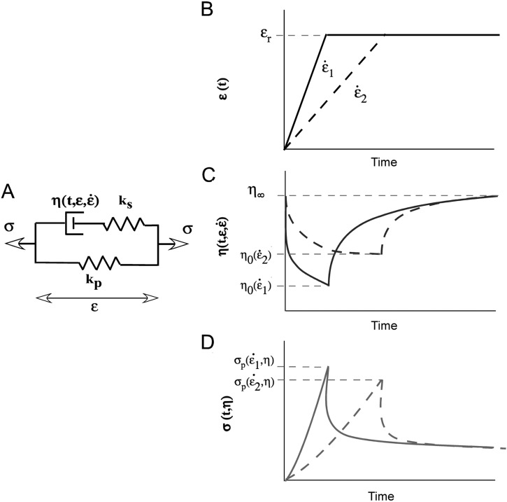
A pseudoplastic model incorporating nonlinear viscosity requires a viscous term that is time, strain and strain rate dependent. This complex viscosity can be incorporated into a single nonlinear element in the 3-element Hill model of passive muscle [6] with a viscous parameter given by $\eta (t,\varepsilon ,\stackrel{·}{\varepsilon })$ (Fig. 1(a)). This approach is similar to the modified superposition method used by Lakes and Vanderby [25]) to describe nonlinearities in ligament behavior, where the relaxation modulus is modified to include a strain dependence. In the pseudoplastic model it is further modified to also include strain rate dependence.

Fig. 1.

Schematic representation of a pseudoplastic model of passive muscle mechanics. Figure 1(a) Modified version of the Hill 3-element model [6]. Spring elements are linear due to the linear stress-strain behavior of mouse muscle fibers and the dashpot is a nonlinear element whose behavior is a function of time, strain and strain rate. Figure 1(b) Schematic of two step strain inputs for a stress relaxation test, one at high strain rate (${\stackrel{·}{\varepsilon }}_1$) and one a low strain rate (${\stackrel{·}{\varepsilon }}_2$). Viscosity in this model is a function of time, strain and strain rate $\eta (t,\varepsilon ,\stackrel{·}{\varepsilon }$)) illustrated graphically in (Fig 1(c)). The shape of the resulting stress relaxation curves are shown in (Fig 1(d )) where the stretch at the higher strain rate results in the higher peak stress ($\sigma ({\stackrel{·}{\varepsilon }}_1,\eta$)).

This model contains linear elastic elements due to the essentially linear stress-strain behavior of mouse EDL fibers [26]. The mathematical form of the strain rate dependence of viscosity can be derived from an equation frequently used in rheology to describe pseudoplastic material behavior (Eq. 1) [27]. A pseudoplastic material exhibits decreasing viscosity with increasing shear-rate (Figs. 1(b) and 1(c)). In this formulation, viscosity ($\eta$) is inversely proportional to strain rate ($\stackrel{·}{\varepsilon }$), and the initial and minimal viscosities are defined by m and ${\eta }_0$ respectively.

$${\eta }_{\mathit{shear}}={\eta }_0+\frac{m-{\eta }_0}{(1+\stackrel{·}{\varepsilon })}$$ (1)

The dependence of viscosity on time during the period of stress relaxation can be explained by pseudoplastic theory. When the shear stress is removed (the material is held at a constant strain) the viscosity returns to the initial, larger value, ${\eta }_{\infty }$, (Figs. 1(b) and 1(c)). This “buildup” is represented by Eq. (2).

$${\eta }_{\mathit{rest}}=\frac{{\tau }^2}{\tau -t\stackrel{·}{\tau }}$$ (2)

Where the function $\tau$ is given by Eq. (3)

$$\tau =\frac{{\eta }_{\infty }{\eta }_0(t^2+(1+2\alpha )t+\alpha )}{{\eta }_0{t}^2+({\eta }_0+2\alpha {\eta }_{\infty })t+\alpha {\eta }_{\infty }}$$ (3)

In this formulation, the increase in viscosity under zero shear load is hyperbolic beginning at a minimal value of ${\eta }_0$ and increasing to a final value of ${\eta }_{\infty }$. The constant $\alpha$ controls the hyperbolic curvature, or the rate at which viscosity increases. Finally, the dependence of the viscous parameters ${\eta }_0$ and $\alpha$ on resting strain can be described by Eq. (4) where ${\varepsilon }_r$ is resting strain and a and b are constants.

$$\begin{array}{c}\multicolumn{1}{c}{{\eta }_0=a{\varepsilon }_r\alpha =b{\varepsilon }_r}\end{array}$$ (4)

With the dependence of viscosity on time, strain and strain rate thus defined, the response of mouse muscle fibers to a stress relaxation test of any rate can be determined by solving the constitutive equation of the 3-element Hill model as piecewise continuous under conditions of shear and rest (Eq. 5).

$$\begin{array}{c}\multicolumn{1}{c}{\stackrel{·}{\sigma }+\frac{k_s}{\eta (t,{\varepsilon }_r,\stackrel{·}{\varepsilon })}\sigma =\frac{k_s{k}_p}{\eta (t,{\varepsilon }_r,\stackrel{·}{\varepsilon })}\varepsilon +(k_s+k_p)\stackrel{·}{\varepsilon },\mathrm{\hspace{1em}\hspace{1em}\hspace{1em}}\mathrm{where}\eta (t,{\varepsilon }_r,\stackrel{·}{\varepsilon })={\eta }_{\mathit{shear}}(\stackrel{·}{\varepsilon })\mathrm{\hspace{1em}\hspace{1em}\hspace{1em}}\mathrm{for}\mathrm{\hspace{1em}\hspace{1em}\hspace{1em}}\stackrel{·}{\varepsilon }>0\eta (t,{\varepsilon }_r,\stackrel{·}{\varepsilon })={\eta }_{\mathit{rest}}(t,{\varepsilon }_r)\mathrm{\hspace{1em}\hspace{1em}\hspace{1em}}\mathrm{for}\mathrm{\hspace{1em}\hspace{1em}\hspace{1em}}\stackrel{·}{\varepsilon }=0}\end{array}$$ (5)

As an example, a commonly used material test for muscle is to perform a single stress relaxation test at a high rate that approximates an instantaneous change in strain. In this approximation, $\mathrm{\eta }$ changes instantaneously to ${\eta }_0$ under shear and Eq. (5) can be solved for the rest case only (Eq. 6).

$$\sigma =k_s\mathit{exp}\left(\frac{-k_{s}t({\mathit{at}}^2+(a+2\alpha b)t+b)}{\mathit{ab}{\varepsilon }_r(t^2+(1+2\alpha )t+\alpha )}\right)+k_p$$ (6)

Model Fitting.

All analysis was performed using Matlab. Solutions to models with instantaneous step strain profiles were exact while solutions to models with ramp strain profiles were solved numerically using a nonstiff initial value ordinary differential equation solver. These solution methods were combined with a nonlinear least-squares parameter-fitting algorithm to optimize the solutions. Initial parameter guesses within a 100-fold range of the solution were shown to result in the same solution, indicating high model robustness.

Results

The most commonly performed test to evaluate the viscoelastic properties of skeletal muscle is a ramp-and-hold stress relaxation test (depicted in Fig. 1(b)) [9,12,16,21,28]. In this test, strain is increased at a fixed rate to a final value at which the muscle is allowed to relax until stress reaches a steady state. Frequently these tests are performed at very high strain rates to approximate instantaneous changes in strain [9,15,16,29]. This infinite-rate assumption simplifies the model fitting process as an exact solution is available for both structural and QLV models. These models can be fit to either a single stress relaxation (a locally linear model) or to stress relaxations over a range of strains. For simplicity, locally linear models will be considered first.

Locally Linear Models.

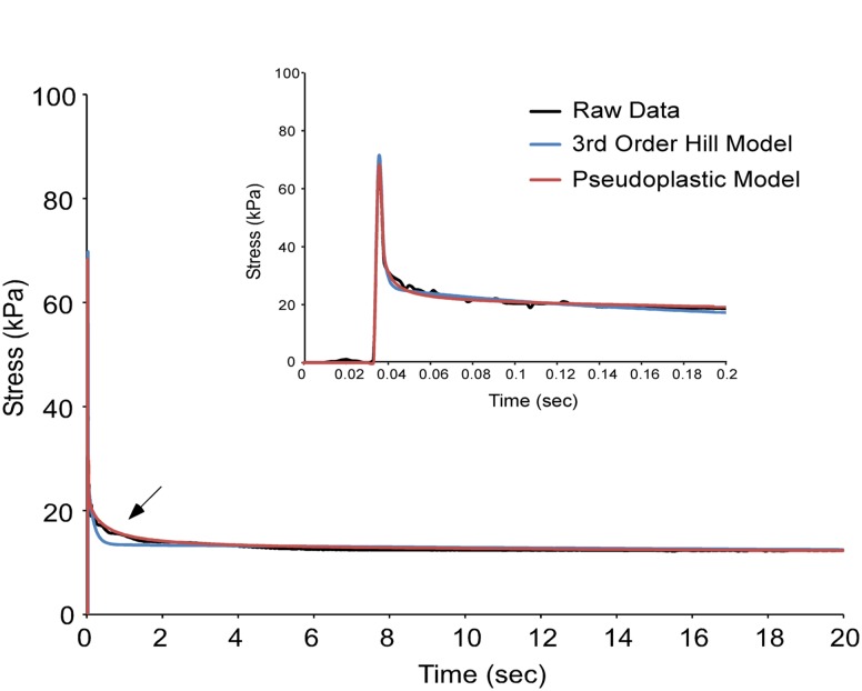
Figure 2 presents data from a stress relaxation test on a mouse EDL fiber at a super-physiological strain rate (20 FL/s) to approximate an instantaneous change in strain. These data were then fit with an $3\mathit{rd}$ order Hill structural model (Appendix A) using the infinite rate assumption. This structural model uses three viscous elements to describe the relaxation process, which results in a distinctive error during the fast phase of relaxation as the model attempts to represent a continuous process with discrete structural elements (arrow). The pseudoplastic model described here assumes a continuous spectrum of relaxation similar to that frequently used in conjunction with QLV models where a single viscous element is allowed to change its viscosity over time [9,30].

Fig. 2.

The pseudoplastic model better represents stress relaxation data from a mouse muscle fiber compared to the 3rd order Hill structural model. The fiber was stretched to 30% FL at 20 FL/s to approximate an instantaneous length change. The pseudoplastic model (red) is a better fit to the raw data (black) than the 3rd order Hill model (blue) during the phase of fast relaxation. Inset shows the data magnified over the first 0.2 s of stress relaxation.

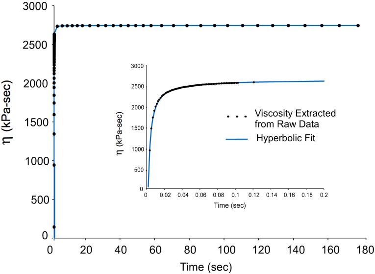
To evaluate how the viscosity of the fiber changes over time during the process of stress relaxation, data from a fiber was fit with individual $1^{\mathit{st}}$ order Hill models at discrete time points during relaxation. The viscosities of these models were then plotted as a function of time during the course of stress relaxation (Fig. 3). The model viscosity increases as a function of time and was best fit by a hyperbolic relationship Eq. (3) (${\mathrm{r}}^2$ = 0.998). Incorporating this relationship into the pseudoplastic model solution for an infinite-rate stress relaxation test (Eq. 6), gives an analytical solution that can be fit to stress relaxation data. Figure 2 illustrates this fit compared to the 3rd order Hill model fit where superior representation of the data can be seen with the pseudoplastic model (arrow) especially during the fast phase of stress-relaxation (${\mathrm{r}}^2$ = 0.949 (3rd order Hill), ${\mathrm{r}}^2$ = 0.987 (pseudoplastic) during 0-2 s). Though both models could be said to yield good fits to the data, the 3rd order Hill model requires 7 independent parameters while the pseudoplastic model requires only 5, optimizing the number of parameters to the goodness of fit.

Fig. 3.

Change in viscosity over time during fiber stress relaxation. Individual data points (black circles) were derived from 1st order Hill fits to the stress relaxation of a fiber at discrete time points. Eq. (3) provided a good fit to the data with an r-squared value of 0.998.

QLV models frequently also incorporate a continuous spectrum of relaxation defined by exponential integrals (Appendix B) and such models require only four independent parameters. However, the exponential integral stress relaxation poorly characterizes mouse fiber data at low strains and thus this model did not represent the experimental data described here as well as either the 3rd order Hill model or the pseudoplastic model (Table 1).

Table 1.

Comparison of the locally linear fits of three models to mouse fiber stress relaxation. Data were taken from 40 total stretches of 5 fibers over the strains and strain rates discussed. Goodness of fit was calculated over the first 2 s of stress relaxation. The pseudoplastic model provides a superior goodness of fit to both the 3rd order Hill model and the QLV model (using exponential integral reduced relaxation).

	# Parameters	Average r-squared
3rd Order Hill Model	7	0.918 $\pm$ 0.035
Exponential Integral Reduced Relaxation	4	0.785 $\pm$ 0.334
Pseudoplastic Model	5	0.958 $\pm$ 0.018

Strain Rate Sensitivity.

The peak stress experienced by a passively ramp-stretched muscle is known to be a function of the rate at which it is strained. Structural models such as the 3rd order Hill model inherently predict high strain rate sensitivity. This is due to the fact that the fastest decay constant (associated with the dashpot with lowest viscosity) will cause significant stress decay during the finite time stress ramp. The magnitude of this decay will increase as strain rate decreases and the amount of time spent in the strain ramp increases. The QLV model predicts the same high strain rate sensitivity since viscosity is only a function of time and thus the 3rd Order Hill model is representative of both responses.

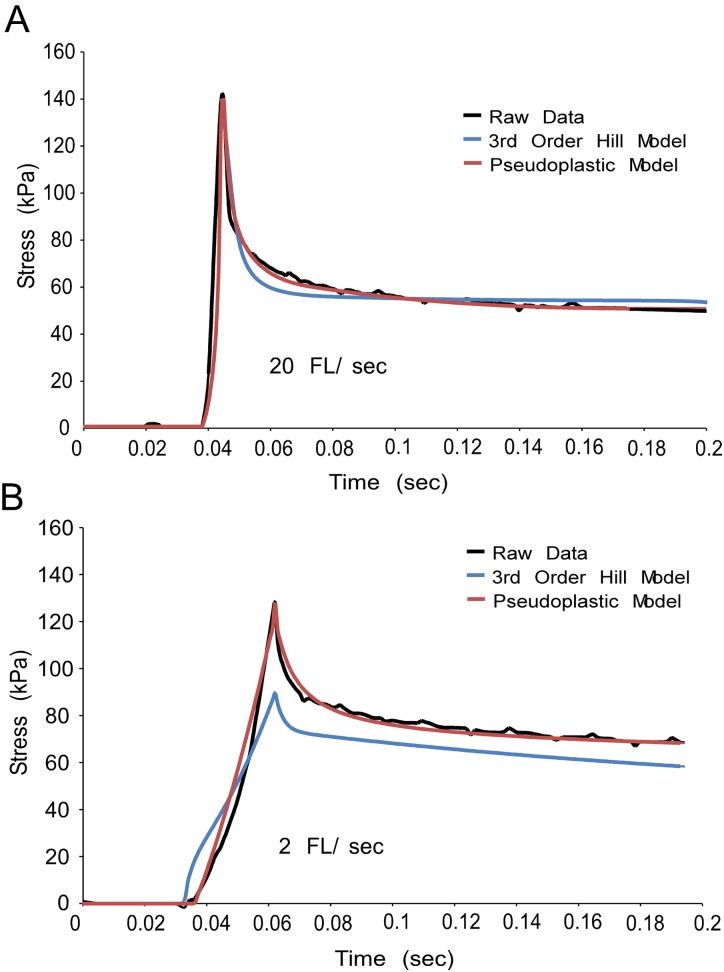
At the strains and strain rates considered here, the mouse muscle fibers were found to be significantly less strain rate sensitive than the 3rd order Hill model predicted. 3rd order Hill model fits to high strain rate data were found to underestimate peak stresses at lower rates by as much as 50%. Figure 4 shows raw data from a single mouse muscle fiber strained to 50% FL at two strain rates. The 3rd order Hill model was fit to 20 FL/s data and then used to predict 2 FL/s data (blue traces). The model is unable to explain the fiber behavior at 2 FL/s, underestimating peak stress by 30%. The difference in strain rate sensitivities between the 3rd order Hill model and mouse muscle fibers was seen at all strains between 10 and 50% FL (data not shown).

Fig. 4.

The pseudoplastic model better represents the strain rate sensitivity of a mouse muscle fiber than the 3rd order Hill structural model. A single mouse muscle fiber was strained to 50% FL at 20 FL/s (Fig. 4(a) and at 2 FL/s (Fig. 4(b)). The 3rd order Hill model (blue) and the pseudoplastic model (red) were fit to raw data (black) at 20 FL/s and then used to predict behavior during a 2 FL/s stretch. The 3rd order Hill model underestimates stress at 2 FL/s, while the pseudoplastic model accurately represents peak stress.

Pseudoplastic theory offers an explanation for this disparity by introducing nonlinearity to the viscosity. The viscosity of a pseudoplastic material decreases inversely proportionally with strain rate during the time the material is subjected to stress. Thus, during the ramp stretch, the material would experience less stress decay, as it would have begun at a high viscosity and only reached the lowest viscosity at the end of the ramp. The pseudoplastic model considered here is able to provide good fits to fiber data at both strain rates with a single set of parameters and an appropriate dependence of viscosity on strain rate (Fig. 4, red traces). Similarly, the pseudoplastic model fit to slow strain rate data is able to well represent faster strain rate data whereas the 3rd order Hill model overpredicts peak stress at the faster rate with parameters based on the slower rate (data not shown).

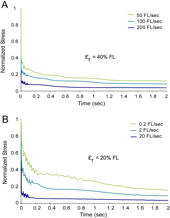
Evidence from mouse muscle fibers suggests that they behave like a pseudoplastic material. It is difficult to measure viscosity in a fiber during shear, but the initial rate of stress relaxation following strain can be used as an indication of the minimum viscosity reached, ${\eta }_0$ [31]. Three stretches of the same fiber are shown, each at a different strain rate ranging from 50 FL/s to 200 FL/s (Fig. 5(a)). The stress is normalized on a scale from zero to one to enable a direct comparison of stress decay rates in different stretches. The stress clearly decays fastest at the highest strain rate indicating the fiber reaches the lowest viscosity under this condition. This behavior is typical of a pseudoplastic material where viscosity decreases with increasing strain rate.

Fig. 5.

Mouse muscle fibers exhibit pseudoplasticity. Figure 5(a) single fiber was strained to 40% FL at three different rates. The fastest rate stretch resulted in the fastest stress decay indicating the lowest viscosity. All strain ramps had the same time interval and the same peak stress. Figure 5(b) single fiber was strained from slack length to 20% FL at three different rates. Again, the fastest stretch had the fastest stress decay, indicative of pseudoplastic behavior. Noise on the traces represents less than 1 mV noise at these low stresses.

The three stretches depicted reached the same final resting strain (40% FL), but the initial strain for each was selected such that the fiber spent the same time under shear load for each case. This was done deliberately to separate pseudoplastic (viscosity as a function of strain rate) effects from thixotropic (viscosity as a function of shear time) effects. Additionally, peak stresses for the three stretches were within 10% of each other, eliminating stress as a compounding factor. The length change to which the fiber was subjected, however, was still variable in this test. Three stretches of the same fiber were again performed at three different strain rates ranging from 0.2 FL/s to 20 FL/s, but this time all strains were from slack length to 20% FL (Fig. 5(b)). Again, the stretch at the highest rate had the fastest relaxation, indicating that it reached the lowest viscosity and suggesting pseudoplastic behavior. Time spent under shear load for each stretch is variable in this data, but the stretch with the longest time (0.2 FL/s) had the slowest relaxation rate and thus the highest viscosity—the opposite of a thixotropic effect.

Superposition.

Stress relaxation tests are usually performed on muscle either from a predefined “slack length” [9,28] or incrementally at set step increments [14,21,29]. Linear models, which are most commonly used, obey the principle of superposition, meaning that that the stress response to reach a given strain is necessarily equal to the net stress responses of any number of intermediate steps to that strain. The QLV model also obeys superposition, and results in similar predictions of peak forces as linear models.

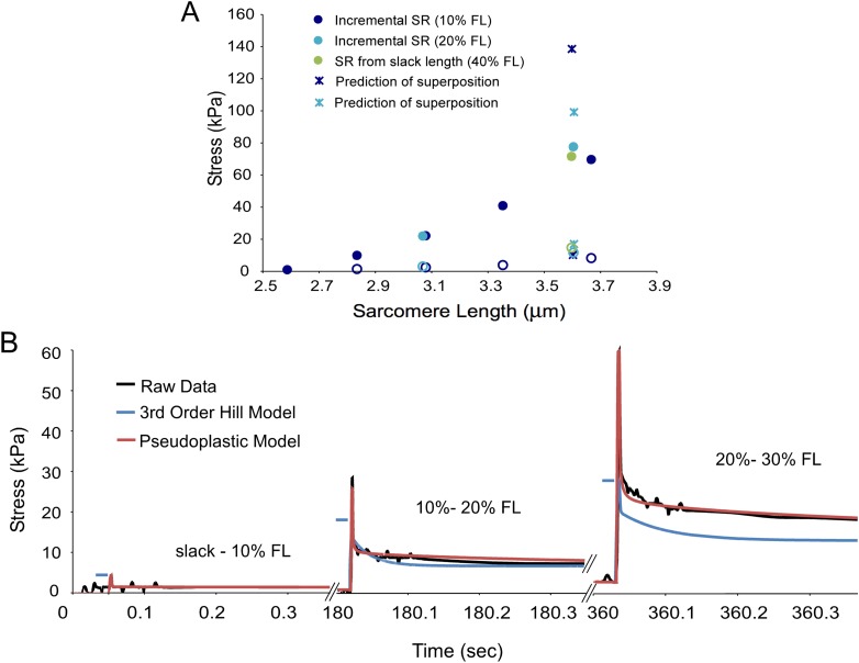
However, experimental data indicate that mouse muscle fibers do not obey the principle of superposition. In fact, the peak stress experienced by fibers seems to be nearly completely a function of the final strain reached regardless of the magnitude of the strain step, an observation also noted by Quaia et al [14]. Peak stress (Fig. 6(a), filled circles) and relaxed stress (Fig. 6(b), open circles) data are shown from a mouse muscle fiber subjected to a variety of stress relaxation tests. In the first test (blue circles), the fiber is strained in 10% FL increments to 40% FL. The peak and relaxed stresses are then respectively summed to yield the superposition prediction of the peak and relaxed stress for a strain from slack length to 40% FL (blue circles), In the second test, the same fiber was strained in increments of 20% FL (turquoise circles) and the superposition prediction was made in the same way (turquoise asterisk). Finally, the fiber was stretched from slack length to 40% FL (green circles). The superposition predictions of relaxed stress are close to the fiber measurement, but the peak superposition predictions overestimate the fiber measurement by 40% and 95% respectively. Thus, superposition is only a reasonable assumption for the relaxed stress measurement. It does not reflect peak stress or stress relaxation behavior.

Fig. 6.

Mouse muscle fibers do not obey superposition. Figure 6(a) Peak (closed circles) and relaxed (open circles) stresses from a single fiber strained incrementally at 10% FL increments (blue) and 20% FL increments (turquoise). These data were used to predict stresses from a stretch from slack to 40% FL based on the principle of superposition (asterisks). Predictions match experimental data for the relaxed stress (open green circle), but overestimate the peak stress by as much as 95% (closed green circle). Figure 6(b) raw stress relaxation data from a fiber stretched in 10% FL increments (black). The 3rd order Hill model is fit to stretches of the same fiber from slack but provides a poor prediction of incremental stress (blue). The pseudoplastic model overcomes the limitations of superposition by adding strain dependent viscous parameters and provides a much better fit (red). Relaxation plots are truncated at 0.3 s to show the initial fast phase of relaxation. Both models converge with the raw data at the fully relaxed stress.

Since a linear model, by definition, obeys the principle of superposition, a fit to stress relaxation data from slack length would be unable to describe incremental stress relaxation data and vice versa. This is true of the 3rd order Hill model and the QLV model, though only the 3rd order Hill fit is shown. Figure 6(b) shows raw incremental stress relaxation data for three consecutive stretches of a mouse muscle fiber (black traces) at 10% FL. The 3rd order Hill model was fit to stress relaxation data from slack length and then used to predict incremental stress relaxation values (blue traces). The model underestimates the raw data by increasing margins with succeeding increments (30% at 20% FL and 50% at 30% FL). Nonlinearities introduced into the dashpot elements of this model may be able to explain some of the muscle fiber's deviation from superposition. If, for instance, the viscosity of the dashpot element increased with increasing resting strain, a stretch from 30% to 40% FL could develop as much stress as a stretch from slack length to 40% FL simply due to its higher initial viscosity.

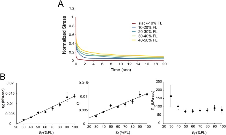
Experimental data indicate that the viscosity of mouse muscle fibers increases with increasing resting strain, as revealed by normalized stress relaxation data from a fiber subjected to a series of incremental stretches from slack length to 50% FL (Fig. 7(a)). Normalized stress decays from the same maximum to the same minimum more slowly as the strain is increased from 0 to 50% FL. If the pseudoplastic model is locally fit to each stretch, the parameters ${\mathrm{\eta }}_0$ and $\mathrm{\alpha }$ both increase as a function of resting strain (${\mathrm{\varepsilon }}_{\mathrm{r}}$). Analysis of the three viscous parameters of the pseudoplastic model as a function of resting strain for incremental stretches of six fibers to 100%FL (Fig. 7(b)), revealed that the parameters ${\mathrm{\eta }}_0$ and $\mathrm{\alpha }$ increase linearly with resting strain (r-squared = 0.97 and 0.95 respectively) while ${\mathrm{\eta }}_{\infty }$ remains essentially constant. With stain dependent viscous parameters (Eq. 4), the pseudoplastic model can characterize the fiber's deviation from superposition (Fig. 6(b), red traces).

Fig. 7.

Viscosity is a function of strain in mouse muscle fibers. Figure 7(a) Normalized stress relaxation data from a single fiber subjected to an incremental stress relaxation test from slack length to 50% FL at 20 FL/s. Stress is decay is slower with increasing strain, indicating fiber viscosity is increasing as a function of resting strain. Figure 7(b) The pseudoplastic model was used to locally fit incremental stress relaxation data from six fibers from slack length to 100% FL at 20 FL/s. Parameters and both increase linearly as a function of resting strain, but remains relatively constant.

Discussion

The purpose of this study was to define the passive mechanical behavior of single fibers from the mouse 5^th toe EDL muscle under a variety of strains and strain rates to evaluate the applicability of a linearly viscous model. The data acquired demonstrate that the viscosity of mouse muscle fibers is not linear as is typically assumed, but rather a more complex function of time, strain and strain rate. A new pseudoplastic model was developed to describe these nonlinearities and was shown to provide an excellent fit to stress relaxation data and to account for the strain rate sensitivity and deviation from superposition observed in the fibers.

The pseudoplastic model was compared with two models frequently used to describe stress relaxation in muscle, the 3rd order Hill model and the QLV model. The pseudoplastic model is an adaptation of the 1st order Hill model to include nonlinearities in viscosity and thus the comparison between this model and the 3rd order Hill model reduces to a comparison between nonlinear and linear viscosity. The 3rd order Hill model is frequently only used locally to obtain parameters from a single high strain rate stress relaxation test in a comparative study where the conditions are the same between groups. Under these conditions, viscosity would be only a function of time and this dependence can be reasonably well approximated by combining linear viscous elements. The more viscous elements combined in parallel, the better fit the Hill model provides. However, the ideal model would describe the maximum amount of data with the minimum number of parameters. Continuing to add viscous elements to the Hill models increases the model complexity. Thus, for the purposes of comparison, the 3rd order Hill model was chosen to balance complexity with goodness of fit. The pseudoplastic model provided a much better fit to the data described here than the 3rd order Hill model with fewer parameters because it allowed the viscosity to change at every time point rather than limiting it to three discrete values.

The QLV model also allows viscosity to be a function of time by mathematically incorporating a continuous spectrum of relaxation into the model. However, a primary tenet of this model is that the relaxation response is separable, i.e., that the relaxation response is not a function of strain. It has been shown in the data presented here and elsewhere [13,14] that this is not the case for muscle. Nekouzadeh et al. [32] developed an extension of the QLV model, which allows relaxation to adapt to strain history and eliminates the requirement for separability. However, both this adaptive QLV model and the original QLV model still obey superposition and thus cannot describe the response of the muscle to incremental stretches [14]. The pseudoplastic model allows the stress relaxation process to be a function of strain and allows fiber viscosity to decrease during stretch, which enables it to explain fiber behavior over all of the strains and strain rates considered here.

Hyperelastic models are also frequently used to model skeletal muscle mechanics especially as they are applied to finite element models. However, these have either neglected the contribution of viscosity or modeled it as linear [18–20] and typically require a large number of parameters. Thus, these models were not used to fit the data described here but could theoretically be modified to include viscous nonlinearities.

Other nonlinear model formulations have been developed and implemented to describe the material behavior of other soft tissues such as ligament with good success [10,25,33]. These models have employed similar strategies to the pseudoplastic model described here where the viscous parameters of a linear model are modified to include nonlinearities. The pseudoplastic model takes the description further; however, allowing the viscous parameters to be continuous and to be functions of strain rate. In addition to describing these dependencies mathematically, it offers a physical explanation for the deviation of fiber behavior from separability and superposition. If muscle is indeed a pseudoplastic material, its viscosity would be continuously changing as intermolecular bonds are continuously formed and broken and it is likely that these interactions change with geometry.

Muscle as a Non-Newtonian Material.

Muscle has long been considered to be non-Newtonian in nature, i.e., it exhibits a viscosity that is not constant. Sinusoidal studies on passive muscles and single fibers show a “short range stiffness” where the sample is initially very stiff but then becomes more compliant as the strain profile continues [34–36]. This observation was attributed to the muscle being thixotropic, or having a viscosity that decreases with time spent under shear load. However, the observation that muscle viscosity decreases under load could also be explained by pseudoplasticity, where the viscosity decreases inversely proportionally to the increase in strain rate. The data presented here suggest that mouse single fibers are pseudoplastic rather than thixotropic, but it is possible that the decrease in viscosity under shear load is a more complex function of both strain rate and time. Quaia et al. [37] created a passive muscle model that incorporates thixotropy, but they noted as well that during relaxation, the stress drops faster following faster elongations, an indication of pseudoplastic behavior.

The mechanism behind this non-Newtonian behavior is not well understood, but the applied stress is supposed to induce reversible microstructural “breakdown,” possibly through bond or network disruption, thus reducing viscosity. After the removal of the stress, the bonds or networks are reformed spontaneously leading to a “rebuilding” of viscosity. In this study, the data suggest that components of the breakdown and rebuilding phases in muscle fibers are functions of strain. It is possible that, as cytoskeletal elements are lengthened and interstitial space is reduced in the fibers, that the kinetics of these phases are altered. For example, as strain increases, it could become more difficult to break the molecular interactions, leading to a smaller decrease in viscosity for a given strain rate (i.e. an increase in ${\mathrm{\eta }}_0$ with strain). The parameter $\alpha$ is also increased with strain, which reflects slower rebuilding, but eventually all interactions are reformed and the fiber is back to a relatively strain insensitive viscosity (${\mathrm{\eta }}_{\infty }$). Another mechanism proposed in the ligament literature is that increased strains result in increased fluid loss, causing the tissue to become more elastic in nature [33], which is certainly a possibility in these skinned fibers where fluid is allowed to flow freely into and out of the cell.

Sources of Passive Viscosity.

Many components of muscle have been proposed to contribute to viscosity including the myoplasm, weakly attached cross-bridges, collagen fibrils, titin and other cytoskeletal proteins [38]. Only muscle fiber viscosity is considered here eliminating any contribution of the extracellular matrix (ECM), but it will be interesting to compare the properties measured here in fibers to bundles and whole muscle. Although fiber elasticity is essentially linear (Fig. 6(a)), the inclusion of ECM at the bundle and whole muscle scale imparts significant nonlinearity [26].

It is likely that, like elasticity, the dependence of viscosity on time, strain and strain rate could change dramatically with scale, aging or disease. Chronic alterations in viscosity may well have a large effect on muscle function and thus sources of viscosity should be considered as potential therapeutic targets. This new pseudoplastic model is a tool to evaluate these changes and their effect on function.

Appendix A

Hill Models of Viscoelasticity.

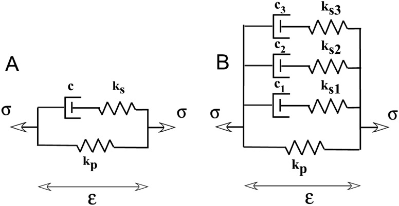
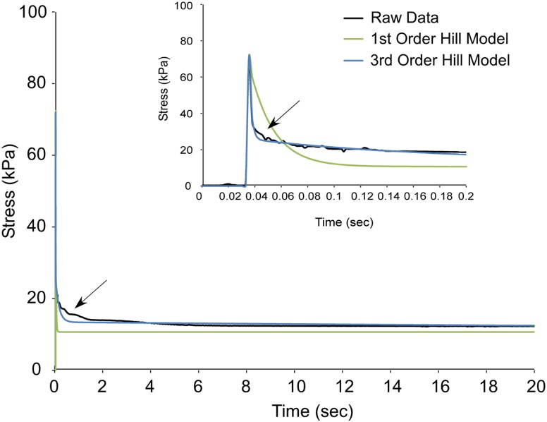
The first and most basic model of muscle viscoelasticity was proposed by A. V. Hill [6]) in 1938 as a contractile element which provides structural damping under passive conditions in series with a spring which provides transient stiffness to the system under conditions of fast stretch. These two elements are placed in parallel with another spring which provides a time-invariant material stiffness (Fig. 8(a)). In the case of passive muscle, this model is equivalent to a standard linear solid model of viscoelasticity, since the contractile element can be represented by a linear dashpot. The Hill model reproduces the basic form of muscle stress relaxation, but fails to accurately reproduce the fast phases of stress decay since it is limited by a single decay rate [9]. Raw data from a mouse muscle fiber during a stress relaxation test to 30% FL at 20 FL/s (Fig. 9, black) reveal that the Hill model (Fig. 9, green) underestimates the decay rate in short time (inset) and overestimates it in long time as it attempts to describe multiple decay rates with one time constant.

To overcome this limitation, the classic Hill model is frequently modified to include additional branches of a dashpot and a series spring [39–41]. These models can include n number of branches, which provide n number of exponential stress decay rates. The stress response of the n^th order Hill model to a strain profile ($\varepsilon$) can be determined by solving the following system of coupled linear differential equations (Eq. 7).

Fig. 8.

Schematics of the classic Hill model of muscle viscoelasticity (A) and the 3rd order Hill model (generalized Maxwell model) (B). The contractile element is represented by a dashpot with damping constant c since only passive muscle mechanics are considered here. The series and parallel springs are represented by linear spring constants of modulus k _s and k _p respectively. The 3rd order Hill model includes two additional branches of dashpot and series spring in parallel, which add two additional time constants to the stress decay during relaxation.

Fig. 9.

The 3rd order Hill model better represents stress relaxation data from a mouse muscle fiber than the 1st order Hill structural model. The fiber was stretched to 30% FL at 20 FL/sec to approximate an instantaneous length change. The 3rd order Hill model (blue) provides a better fit to the raw data (black) than the 1st order Hill model (green) during the phase of fast relaxation. Inset shows the data magnified over the first 0.2 seconds of stress relaxation.

$$\begin{array}{c}\multicolumn{1}{c}{\stackrel{·}{\sigma }=k_p\stackrel{·}{\varepsilon }+\sum _{i=1}^n{k}_{\mathit{si}}{\stackrel{·}{\varepsilon }}_i}\\ \multicolumn{1}{c}{{\stackrel{·}{\varepsilon }}_i=\stackrel{·}{\varepsilon }-\frac{k_{\mathit{si}}}{c_i}{\varepsilon }_i}\end{array}(7)$$ (7)

As additional branches are added to the classic Hill model, it is better able to represent the shape of the stress decay. However, each additional branch adds an equation to the system, increasing the complexity and the number of parameters. If too many branches are added, some of the parameters become redundant and thus difficult to interpret. Ideally, the minimum number of branches would be added in order to improve the fit to some predetermined tolerance. For the data considered here, the 3rd order Hill model best meets this goal, yielding an r-squared value of 0.98 with only two additional branches. The 3rd order Hill model fit to the raw data (Fig. 9, blue) provides a much better representation of the stress decay than the classic $1^{\mathit{st}}$ order Hill model though still misestimating the decay rates at some points (arrow).

Appendix B

The Quasi-Linear Viscoelastic Theory.

Quasi-linear viscoelasticity (QLV) was developed to provide a more general formulation of viscoelasticity, which would be more flexible in its ability to describe nonlinear elastic materials. The basic tenet of this model is that viscoelastic behavior of soft tissues is composed of a nonlinear elasticity superimposed on a linear relaxation. This property is stated mathematically in Eq. (8) where K($\varepsilon$,t) is the relaxation function describing the response of the tissue to an infinite rate step elongation from 0 to $\varepsilon$ G(t) is the reduced relaxation function which describes the normalized stress decay and $T^{(e)}$ ($\varepsilon$) is the elastic response and is a function of strain alone.

$$K(\varepsilon ,t)=G(t)T^{(e)}(\varepsilon )(8)$$ 8

The elastic function is typically either a polynomial or an exponential similar to the springs in nonlinear versions of structural models. The reduced relaxation function can take many forms, but the two most common use a sum of exponentials [13] or an exponential integral formulation [9]. The relaxation function that uses G(t) as a sum of exponentials reduces to the solution of the generalized Hill model for infinite rate step strains and thus will not be considered separately. The other commonly used form of the reduced relaxation function is given by Eq. (9), where $E_1$ (t) is the exponential integral [30].

$$G(t)=\frac{1+c[E_1\left(\frac{t}{{\tau }_2}\right)-E_1\left(\frac{t}{{\tau }_1}\right)]}{1+c\mathit{ln}\left(\frac{{\tau }_2}{{\tau }_1}\right)}(9)$$ (9)

The derivation of the exponential integral formulation of stress relaxation is based on the assumption of a continuous spectrum of relaxation. Essentially, instead of having a discrete number of individual decay rates (${\tau }_i$), $\tau$ is allowed to be a continuous variable changing in time from ${\tau }_1$ to ${\tau }_2$.

Eq. (8) applies only to stress responses to instantaneous step changes in strain or approximations thereof, i.e., the infinite rate assumption. It is a specific case of a more general formulation given by Eq. (10).

$$T(t)={\int }_{-\infty }^{t}G(t-\tau )\frac{\partial T^{(e)}[\varepsilon (\tau )]}{\partial \varepsilon }\frac{\partial \varepsilon (\tau )}{\partial \tau }d\tau (10)$$ (10)

To describe the response of a tissue to a generic elongation history, this equation makes use of the superposition principle. It represents a generic response as an infinite sum of relaxation responses to infinitesimally small step-changes in strain. Thus, this model requires that relaxation be a function of time only and that the sample obey superposition.

References

- [1]. Foidart, M. , Foidart J. M., and Engel, W. K. , 1981, “Collagen Localization in Normal and Fibrotic Human Skeletal Muscle,” Arch Neurol., 38, pp. 152–157. [DOI] [PubMed] [Google Scholar]
- [2]. Gao, Y. , Kostrominova, T. Y. , Faulkner, J. A. , and Wineman, A. S. , 2008, “Age-Related Changes in the Mechanical Properties of the Epimysium in Skeletal Muscles of Rats,” J. Biomech., 41, pp. 465–469. 10.1016/j.jbiomech.2007.09.021 [DOI] [PMC free article] [PubMed] [Google Scholar]
- [3]. Smith, L. R. , Lee, K. S. , Ward, S. R. , Chambers, H. G. , and Lieber, R. L. , 2011b, “Hamstring Contractures in Children With Spastic Cerebral Palsy Result from a Stiffer Extracellular Matrix and Increased In Vivo Sarcomere Length,” J. Physio., 589, pp. 2625–2639. 10.1113/jphysiol.2010.203364 [DOI] [PMC free article] [PubMed] [Google Scholar]
- [4]. Gajdosik, R. L. , 2001, “Passive Extensibility of Skeletal Muscle: Review of the Literature With Clinical Implications,” Clin. Biomech. (Bristol, Avon), 16, pp. 87–101. 10.1016/S0268-0033(00)00061-9 [DOI] [PubMed] [Google Scholar]
- [5]. Levin, A. W. J. , 1927, “The Viscous Elastic Properties of Muscle,” Proc. R. Soc., London, Ser. B, 101, pp. 218–243. 10.1098/rspb.1927.0014 [DOI] [Google Scholar]
- [6]. Hill, A. V. , 1938, “The Heat of Shortening and the Dynamic Constants of Muscle,” Proc. R. Soc., London, Ser. B, 126, pp. 136–195. 10.1098/rspb.1938.0050 [DOI] [Google Scholar]
- [7]. Buchthal, F. , Kaiser, E. , and Rosenfalk, P. , 1951, “The Rheology of the Cross-Striated Muscle Fiber With Particular Reference to Isotonic Conditions,” Dan. Biol. Med., 21, pp. 1–302. [Google Scholar]
- [8]. Glantz, S. A. , 1977, “A Three-Element Description for Muscle With ViscoElastic Passive Elements,” J. Biomech., 10, pp. 5–20. 10.1016/0021-9290(77)90025-2 [DOI] [PubMed] [Google Scholar]
- [9]. Best, T. M. , McElhaney, J. , Garrett, W. E. Jr., and Myers, B. S. , 1994, “Characterization of the Passive Responses of Live Skeletal Muscle Using the Quasi-Linear Theory of Viscoelasticity,” J. Biomech., 27, pp. 413–419. 10.1016/0021-9290(94)90017-5 [DOI] [PubMed] [Google Scholar]
- [10]. Thornton, G. M. , Oliynyk, A. , Frank, C. B. , and Shrive, N. G. , 1997, “Ligament Creep Cannot Be Predicted from Stress Relaxation at Low Stress: A Biomechanical Study of the Rabbit Medial Collateral Ligament,” J. Orthop. Res., 15, pp. 652–656. 10.1002/jor.v15:5 [DOI] [PubMed] [Google Scholar]
- [11]. Provenzano, P. , Lakes, R. , Keenan, T. , and Vanderby, R. Jr ., 2001, “Nonlinear Ligament Viscoelasticity,” Ann. Biomed. Eng., 29, pp. 908–914. 10.1114/1.1408926 [DOI] [PubMed] [Google Scholar]
- [12]. Bagni, M. A. , Cecchi, G. , Colombini, B. , and Colomo, F. , 1999, “Mechanical Properties of Frog Muscle Fibres at Rest and During Twitch Contraction,” J. Electromyogr Kinesiol., 9, pp. 77–86. 10.1016/S1050-6411(98)00039-X [DOI] [PubMed] [Google Scholar]
- [13]. Van Loocke, M. , Lyons, C. G. , and Simms, C. K. , 2008, “Viscoelastic Properties of Passive Skeletal Muscle in Compression: Stress-Relaxation Behaviour and Constitutive Modelling,” J. Biomech., 41, pp. 1555–1566. 10.1016/j.jbiomech.2008.02.007 [DOI] [PubMed] [Google Scholar]
- [14]. Quaia, C. , Ying, H. S. , and Optican, L. M. , 2009b, “The Viscoelastic Properties of Passive Eye Muscle in Primates II: Testing the Quasi-Linear Theory,” PloS one, 4, e6480. [DOI] [PMC free article] [PubMed] [Google Scholar]
- [15]. Anderson, J. , Li, Z. , and Goubel, F. , 2002, “Models of Skeletal Muscle to Explain the Increase in Passive Stiffness in Desmin Knockout Muscle,” J. Biomech., 35, pp. 1315–1324. 10.1016/S0021-9290(02)00170-7 [DOI] [PubMed] [Google Scholar]
- [16]. Wolff, A. V. , Niday, A. K. , Voelker, K. A , Call, J. A. , Evans, N. P. , Granata, K. P. , and Grange, R. W. , 2006, “Passive Mechanical Properties of Maturing Extensor Digitorum Longus are not Affected by Lack of Dystrophin,” Muscle Nerve, 34, pp. 304–312. 10.1002/mus.v34:3 [DOI] [PubMed] [Google Scholar]
- [17]. Navajas, D. , Mijailovich, S. , Glass, G. M. , Stamenovic, D. , and Fredberg, J. J. , 1992, “Dynamic Response of the Isolated Passive Rat Diaphragm Strip,” J. Appl. Physiol., 73, pp. 2681–2692. [DOI] [PubMed] [Google Scholar]
- [18]. Blemker, S. S. , and Delp, S. L. , 2005, “Three-Dimensional Representation of Complex Muscle Architectures and Geometries,” Ann. Biomed. Eng., 33, pp. 661–673. 10.1007/s10439-005-1433-7 [DOI] [PubMed] [Google Scholar]
- [19]. Odegard, G. M. , Donahue, T. L. , Morrow, D. A. , and Kaufman K. R., 2008, “Constitutive Modeling of Skeletal Muscle Tissue With an Explicit Strain-Energy Function,” J. Biomech. Eng., 130, p. 061017. 10.1115/1.3002766 [DOI] [PMC free article] [PubMed] [Google Scholar]
- [20]. Lu, Y. T. , Zhu, H. X. , Richmond, S. , and Middleton, J. , 2010, “A Visco-Hyperelastic Model for Skeletal Muscle Tissue Under High Strain Rates,” J. Biomech., 43, pp. 2629–2632. 10.1016/j.jbiomech.2010.05.030 [DOI] [PubMed] [Google Scholar]
- [21]. Shah, S. B. , Davis, J. , Weisleder, N. , Kostavassili, I. , McCulloch, A. D. , Ralston, E. , Capetanaki, Y. , and Lieber R. L., 2004, “Structural and Functional Roles of Desmin in Mouse Skeletal Muscle During Passive Deformation,” Biophys. J., 86, pp. 2993–3008. 10.1016/S0006-3495(04)74349-0 [DOI] [PMC free article] [PubMed] [Google Scholar]
- [22]. Shah, S. B. , and Lieber, R. L. , 2003, “Simultaneous Imaging and Functional Assessment of Cytoskeletal Protein Connections in Passively Loaded Single Muscle Cells,” J. Histochem. Cytochem., 51, pp. 19–29. 10.1177/002215540305100104 [DOI] [PubMed] [Google Scholar]
- [23]. James, R. S. , Altringham, J. D. , and Goldspink, D. F. , 1995, “The Mechanical Properties of Fast and Slow Skeletal Muscles of the Mouse in Relation to their Locomotory Function,” J. Exp. Biol., 198, pp. 491–502. [DOI] [PubMed] [Google Scholar]
- [24]. Smith, L. R. , Gerace-Fowler, L. , and Lieber, R. L. , 2011a, “Muscle Extracellular Matrix Applies a Transverse Stress on Fibers With Axial Strain,” J Biomech., 44, pp. 1618–1620. 10.1016/j.jbiomech.2011.03.009 [DOI] [PMC free article] [PubMed] [Google Scholar]
- [25]. Lakes, R. S. , and Vanderby, R. , 1999, “Interrelation of Creep and Relaxation: A Modeling Approach for Ligaments,” J. Biomech. Eng., 121, pp. 612–615. 10.1115/1.2800861 [DOI] [PubMed] [Google Scholar]
- [26]. Meyer, G. A. , and Lieber, R. L. , 2011, “Elucidation of Extracellular Matrix Mechanics from Muscle Fibers and Fiber Bundles,” J. Biomech., 44, pp. 771–773. 10.1016/j.jbiomech.2010.10.044 [DOI] [PMC free article] [PubMed] [Google Scholar]
- [27]. Sisko, A. W. , 1958, “The Flow of Lubricating Greases,” Ind. Eng. Chem., 50, pp. 1789–1792. 10.1021/ie50588a042 [DOI] [Google Scholar]
- [28]. Ranatunga, K. W. , 2001, “Sarcomeric Visco-Elasticity of Chemically Skinned Skeletal Muscle Fibres of the Rabbit at Rest,” J. Muscle Res. Cell Motil., 22, pp. 399–414. 10.1023/A:1014502610259 [DOI] [PubMed] [Google Scholar]
- [29]. Bensamoun, S. , Stevens, L. , Fleury, M. J. , Bellon, G. , Goubel, F. , and Ba Tho Ho, M. C., 2006, “Macroscopic-Microscopic Characterization of the Passive Mechanical Properties in Rat Soleus Muscle,” J. Biomech., 39, pp. 568–578. 10.1016/j.jbiomech.2004.04.036 [DOI] [PubMed] [Google Scholar]
- [30]. Fung, Y. C. , 2004, Biomechanics: Mechanical Properties of Living Tissues, Springer, New York. [Google Scholar]
- [31]. Doehring, T. C. , Carew, E. O. , and Vesely, I. , 2004, “The Effect of Strain Rate on the Viscoelastic Response of Aortic Valve Tissue: A Direct-Fit Approach,” Ann. Biomed. Eng., 32, pp. 223–232. 10.1023/B:ABME.0000012742.01261.b0 [DOI] [PubMed] [Google Scholar]
- [32]. Nekouzadeh, A. , Pryse, K. M. , Elson E. L., and Genin, G. M. , 2007, “A Simplified Approach to Quasi-Linear Viscoelastic Modeling,” J. Biomech., 40, pp. 3070–3078. 10.1016/j.jbiomech.2007.03.019 [DOI] [PMC free article] [PubMed] [Google Scholar]
- [33]. Provenzano, P. P. , Lakes, R. S. , Corr, D. T. , and Vanderby, R. Jr. , 2002, “Application of Nonlinear Viscoelastic Models to Describe Ligament Behavior,” Biomech. Model. Mechanobiol., 1, pp. 45–57. 10.1007/s10237-002-0004-1 [DOI] [PubMed] [Google Scholar]
- [34]. Hill, D. K. , 1968, “Tension Due to Interaction Between the Sliding Filaments in Resting Striated Muscle: The Effect of Stimulation,” J. Physiol., 199, pp. 637–684. [DOI] [PMC free article] [PubMed] [Google Scholar]
- [35]. Wiegner, A. W. , 1987, “Mechanism of Thixotropic Behavior at Relaxed Joints in the Rat,” J. Appl. Physiol. , 62, pp. 1615–1621. [DOI] [PubMed] [Google Scholar]
- [36]. Lakie, M. , and Robson, L. G. , 1988, “Thixotropy: The Effect of Stretch Size in Relaxed Frog Muscle,” Q. J. Exp. Physiol., 73, pp. 127–129. [DOI] [PubMed] [Google Scholar]
- [37]. Quaia, C. , Ying, H. S. , and Optican, L. M. , 2010, “The Viscoelastic Properties of Passive Eye Muscle in Primates III: Force Elicited by Natural Elongations,” PloS One, 5, e9595. [DOI] [PMC free article] [PubMed] [Google Scholar]
- [38]. Moss, R. L. , and Halpern, W. , 1977, “Elastic and Viscous Properties of Resting Frog Skeletal Muscle,” Biophys. J., 17, pp. 213–228. 10.1016/S0006-3495(77)85651-8 [DOI] [PMC free article] [PubMed] [Google Scholar]
- [39]. Ito, D. , Tanaka, E. , and Yamamoto, S. , 2010, “A Novel Constitutive Model of Skeletal Muscle Taking Into Account Anisotropic Damage,” J. Mech. Behav. Biomed. Mater., 3, pp. 85–93. 10.1016/j.jmbbm.2009.05.001 [DOI] [PubMed] [Google Scholar]
- [40]. Zhang, W. , Chen, H. Y. , and Kassab, G. S. , 2007, “A Rate-Insensitive Linear Viscoelastic Model for Soft Tissues,” Biomaterials, 28, pp. 3579–3586. 10.1016/j.biomaterials.2007.04.040 [DOI] [PMC free article] [PubMed] [Google Scholar]
- [41]. Quaia, C. , Ying, H. S. , Nichols, A. M. , and Optican, L. M. , 2009a, “The Viscoelastic Properties of Passive Eye Muscle in Primates I: Static Forces and Step Responses,” PloS One, 4, e4850. 10.1371/journal.pone.0004850.g001 [DOI] [PMC free article] [PubMed] [Google Scholar]