Transfer Learning of Classification Rules for Biomarker Discovery and Verification from Molecular Profiling Studies

Abstract

We present a novel framework for integrative biomarker discovery from related but separate data sets created in biomarker profiling studies. The framework takes prior knowledge in the form of interpretable, modular rules, and uses them during the learning of rules on a new data set. The framework consists of two methods of transfer of knowledge from source to target data: transfer of whole rules and transfer of rule structures. We evaluated the methods on three pairs of data sets: one genomic and two proteomic. We used standard measures of classification performance and three novel measures of amount of transfer. Preliminary evaluation shows that whole-rule transfer improves classification performance over using the target data alone, especially when there is more source data than target data. It also improves performance over using the union of the data sets.

1. Introduction

Molecular profiling data is used extensively to learn classifiers, such as rule models, and discover biomarkers for early detection, diagnosis and prognosis of diseases. Biomarkers are also critical for furthering understanding of disease mechanisms and creating treatments. The aim in biomarker discovery is to find a small set of measured variables that can be used to accurately predict a disease state. This is particularly challenging because typically we must choose among tens or hundreds of thousands of variables, representing molecules in complex mixtures, often with high measurement error. Also, data sets are typically very small, usually tens or hundreds of patients in a study. All these factors make statistical analyses more error-prone.

Fortunately, there are often multiple similar studies, each producing a data set. In order to draw on all the available data, researchers typically analyze each data set separately, then compare the biomarkers discovered [1, 2]. However, this is sub-optimal because the analysis is still done on the separate small data sets. A simple way to combine the data is to use the union of the data sets. But such attempts are typically confounded by variability in sample processing and by systematic measurement error specific to each data set. For example, the same numerical measurement might mean a high abundance of some protein in one data set but low abundance in another data set.

We propose a novel framework for transfer learning, called Transfer Rule Learner (TRL), that is particularly well-suited to biomarker discovery. Transfer learning is the use of data from one learning task to help in learning another task [3]. Pan and Yang [4] offer a survey of transfer learning. Various methods for transfer learning have been applied to various domains, such as part-of-speech tagging [5] and leaf classification [6]. Transfer learning for biomarker discovery is promising because previous studies have found reproducibility of information collected in different experimental sessions when using the same protocols [1, 2]. Unfortunately, many transfer learning frameworks typically produce classifiers that are difficult for human users to understand or that use many variables [3, 5], which makes them less useful for biomarker discovery. Unlike other transfer learning methods, TRL transfers knowledge in the form of modular, interpretable classification rules, and uses them to seed learning of a new classifier on a new data set. Rule learning has the advantage that variable selection is embedded in the learning algorithm, and the new model uses only a few of the many measured variables to explain the data.

TRL is an extension of the classification rule learning algorithm RL [7], which been used successfully to solve biomedical problems for more than three decades [8, 9, 10, 11] and in the past decade has been adapted and used for biomarker profiling [12, 13, 14, 15, 16, 17].

We demonstrate our method on 5 clinical data sets, and find that more often than not, transfer learning improves performance over using one data set alone, and even more often over learning on the union of the data sets. We evaluate the methods using standard performance measures and three novel measures of transfer. To our knowledge, this is the first effort to apply transfer of rules or rule structure between related biomedical data sets.

2. Materials and Methods

Our transfer learning framework is based on the classification rule learner RL [7]. Models learned by RL are simple to understand and can represent non-linear relationships. RL covers data with replacement (see 2.1), which is beneficial when training data are scarce.

Figure 1 shows an overview of our transfer learning approach. A source data set is used to train a set of prior rules that are then used as seeds for learning on the target data. Section 2.1 provides a brief overview of RL, which is useful in understanding transfer learning with TRL described in Sections 2.2–2.4.

Figure 1.

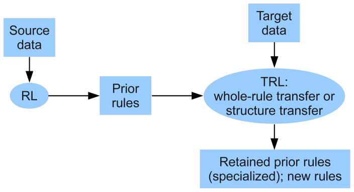
The TRL framework.

2.1. Rule Learning with RL

RL is a classification learning algorithm that outputs a rule-based classifier. RL’s input is a set of training data instances, where each instance is a vector of values for the input variables, and a class value. The learned classifier comprises a set of rules of the form:

IF <antecedent> THEN <consequent>

where the antecedent consists of a conjunction of one or more variable-value pairs (conjuncts), and the consequent is a prediction of the class variable. For example, a rule learned from proteomic mass spectra might be:

IF ((mz_2.05 = High) AND (mz_9.65 = Low)) THEN Class = Control

which is interpreted as “if the variable for m/z 2.05 kilo Daltons (kDa) has a value in the High range and the m/z 9.65 has a value in the Low range, then predict the class value Control.” Values such as Low and High represent intervals of real numbers that result from discretizing the variables before training with RL. (See Section 2.2.) A rule is said to cover or match a data instance if each variable value of the instance is in the range specified in the rule antecedent. RL covers data with replacement, which means that multiple rules are allowed to cover the same training instance. This is unlike most other classification rule and tree learning algorithms, such as C4.5 [18] and CART [19], which cover data without replacement, so that each data instance is covered by only one rule. In small sample size data sets, covering with replacement allows RL to utilize more of the available evidence for each rule when computing the generalizability of the rule.

The classifier also includes an evidence gathering method for breaking ties when the antecedents of several rules are met but their consequents are different. We use the default evidence gathering method: voting weighted by the rules’ certainty factor values.

RL is shown in Algorithm 1. The input is a set of data instance vectors and a set of values for the learning parameters specified by the user. The parameters define constraints on the acceptable rules in terms of a number of quantities defined with respect to a rule and a data set. The constraints are minimum coverage, minimum certainty factor value, maximum false positive rate, and inductive strengthening. Coverage is the fraction of training examples for which the rule antecedent is satisfied. An additional parameter is the certainty factor function. The Certainty factor function (CF) is a measure of the rule’s accuracy; several alternative certainty factor functions are defined and implemented in RL, and the specific function to use can be specified as a parameter to the algorithm. As a CF function, we used the true positive rate: the number of examples the rule predicts correctly divided by the number of examples it matches. False positive rate is the number of examples the rule predicts incorrectly divided by the number of examples it matches. Inductive strengthening is a bias toward training new rules that cover uncovered training instances. Specifically, the parameter specifies the minimum number of previously uncovered examples that a proposed rule must cover. The smaller this number, the larger the overlap of instances covered by different rules. Because RL covers data with replacement, using some non-zero inductive strengthening helps to learn a more generalizable model. Maximum conjuncts is the maximum number of variable-value pairs allowed in the antecedent of any rule.

Algorithm 1.

TRL. Differences from RL are underlined. Function import() takes a list of prior rules and removes from them any variables that do not appear in the data set. satisfies() checks if the rule satisfies the user-specified constraints. The second call to satisfies() checks only the minimum-coverage constraint because coverage of any specialized rule will be equal or smaller. specialize() creates all non-redundant specialized rules by adding to the original rule antecedent single variable-value pairs from the data set.

Input: data, a set of training instance vectors

Input: priorRules, a list of prior rules

Parameters: constraints, constraints on acceptable rules

Parameters: minCoverage, minimum-coverage constraint

beam ← import(priorRules) + [∅ ⇒ class1, ∅ ⇒ class2…];

beam ← sort(beam);

model ← [];

while beam is not empty do

beamnew ← [];

for each rule ∈ beam do

if satisfies(rule, constraints, data) then

model ← model + [rule ];

beamnew ← beamnew + specialize(rule);

else if satisfies(rule, minCoverage, data) then

beamnew ← beamnew + specialize(rule);

end

beam ← sort(beamnew);

end

end

Return model

The algorithm proceeds as a heuristic beam search through the space of rules from general to specific [20]. Starting with all rules containing no variable-value pairs, it iteratively specializes the rules by adding conjuncts to the antecedent. It evaluates the rules and inserts promising rules onto the beam, sorted by decreasing certainty factor value. Beam search is used to limit the running time and space of the algorithm.

2.2. Transfer of Rules

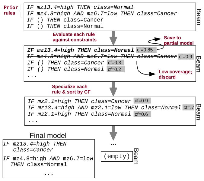
The transfer scheme we propose is to load the prior rules into the beam along with the initial rules, before the first evaluate-specialize iteration. Figure 2 illustrates the algorithm.

Figure 2.

Illustration of the TRL algorithm.

RL’s input data must be discrete, that is, each variable has a small number of values in the data. Many molecular profiling methods create real-valued data, so these data must be discretized before use with RL; that is, for each continuous (real-valued) variable, we must partition the set of real numbers into some small set of intervals, and substitute each observed value of the variable by its corresponding interval. What intervals are chosen in the partition affects the usefulness of the variable in predicting the class variable. Because the variable might have a different distribution in the source data than in the target data, the optimal discretization in each case might also differ. However, it is important for rule transfer that a variable in a prior rule has the same number of intervals in the target data as in the source data. This is because in this case there is a clear mapping between the two sets of intervals: the interval “Low” in the source data corresponds to “Low” in the target data, and so on. The end-points of corresponding intervals might differ, due to the different distribution of values in the two data sets; but this does not matter because transfer learning aims to make use of the commonalities between the two distributions.

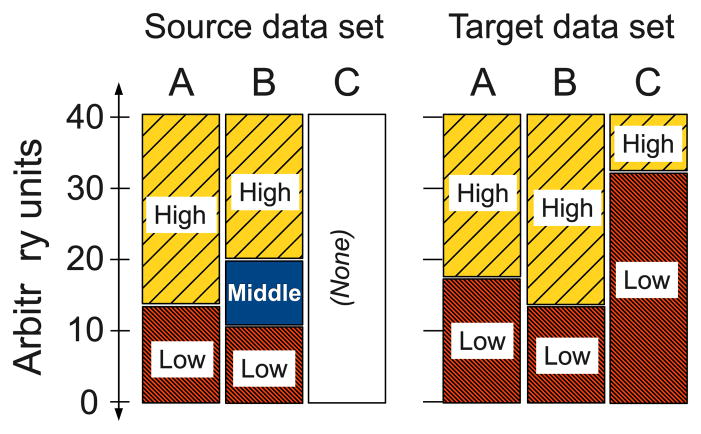
A difficulty arises if the number of intervals differs between source and target, because in that case a value in a prior rule does not have a clear meaning in the target data. For example, suppose a variable A has intervals High, Middle and Low in the source data but only High and Low in the target data (see Figure 3). How should we transfer a rule that has A=Middle in its antecedent? To address this issue, we can either apply the same discretization to both source and target data and transfer whole rules; or we can discretize the data sets separately, and transfer only the “structure” of the prior rules, without the variable values (rule structure transfer); this is done by instantiating the new discrete values for each variable. These approaches are discussed in Sections 2.3 and 2.4 respectively.

Figure 3.

Illustration of discretization issues. Variable A has the same number of discrete values, in the source data and the target data; although the intervals have different endpoints, there is a clear mapping between these sets values. Variables B and C have different numbers of values, and so pose a challenge for transfer.

For discretizing, we used EBD [21, 17]. EBD is a univariate supervised discretizer that uses a Bayesian score to evaluate discretizations for each continuous-valued variable, and runs efficiently on high-dimensional data such as molecular profiling data. EBD performed favorably compared to Fayyad and Irani’s MDLPC [22], which is efficient and commonly-used state-of-the-art method [23]. EBD tended to perform better with rule learners such as RL that learn rules having many attributes in the antecedent. It utilizes a Poisson prior, and by default we set the Poisson parameter λ = 1, so that the mean and variance of the number of cut points has an expected value of 1. Having a single cut point is equivalent to having two intervals, High and Low.

A further consideration is how prior rules will affect RL’s search process. This is discussed in Section 2.5.

2.3. Whole-Rule Transfer

The simplest way to avoid possible differences in the discretization between source and target is to ensure that they are discretized identically. Specifically, we discretized the target data and imposed the same discretization on the source before running RL to compute prior rules. This guarantees that there is a clear mapping between values in the two data sets, even if it means that the prior rules will be less accurate on the target data.

2.4. Rule Structure Transfer

As mentioned in Section 2.2, it might not be optimal to apply the same discretization to the source and target data sets, due to systematic differences between them. For example, two sets of proteomic mass spectra often have different baseline signals caused by the state of the measurement equipment. Even after post-processing such as baseline subtraction, numerical values in one data set might not correspond to numerical values in the other. Ideally, the data sets can be discretized separately to find an optimal discretization for each variable in each data set. However, this might result in a different number of discrete values for a variable in the two data sets, and therefore no clear mapping between values for transfer learning.

To address this problem, we instantiate each prior rule with all possible target values for its variables. In a sense, this means transferring the just the “structure” of the rule without the variable values.

For example, a prior rule:

IF (mz_7.23 = High) THEN (Group = Cancer)

is converted to a prior rule structure:

IF (mz_7.23 = ?) THEN (Group = ?)

The rule is then instantiated from the target data discretization as:

IF (mz_7.23 = High) THEN (Group = Cancer)
IF (mz_7.23 = Low) THEN (Group = Cancer)
IF (mz_7.23 = High) THEN (Group = Healthy)
IF (mz_7.23 = Low) THEN (Group = Healthy)

We consider all class values in addition to all discrete variable values because that more completely represents the possible relationships in the target data.

Transferring rule structure has the additional advantage that the source data set is not needed during the transfer learning. Thus, the prior rules can be used when the source data set is not available, for example by extracting them from literature. For example, serum amyloid A (SAA) has been reported as a serum biomarker for lung cancer [24]. Prior rules could be formulated from known m/z values for this marker, for example by using the EPO-KB data base of biomarker-to-protein links [25].

2.5. Effect of Transfer on RL’s Search Process

As explained in Section 2.1, to avoid overfitting, RL checks that any new rules added to the model cover at least δ previously uncovered training instances, where δ is the inductive strengthening parameter. When prior rules are added to the beam, they may cover some target data instances that would be covered by better performing rules learned in the absence of the prior rules. Thus, the prior rules might displace these better rules from the model and so reduce its classification performance. To reduce this effect, we created a variation of the algorithm that we called “nc” (for “no-covering”). In this variation, the target data instances covered by prior rules are not considered as “covered” for purposes of inductive strengthening. Note that prior rules retained in the classifier can still influence the predictions, and therefore the performance, of the classifier.

2.6. Experiments

We compared the four transfer methods to the baseline condition of learning on the target data set alone, based on classification performance. We also compared the four methods with each other in terms of the three measures of amount of information transferred. Using the data sets, we created two experimental setups, namely inter-set transfer and intra-set transfer. Using cross-validation, we evaluated the methods on three pairs of data sets (see Table 1): one of gene expression and two of protein profiling using SELDI TOF MS.

Table 1.

Data sets used in the experiments. Horizontal lines delimit pairs of data sets where each data set was used once as the target when the other one was the source. “Size” is number of clinical samples from each class.

Type	Disease	Name	Size	Ref.
Genomic	Leukemia	Train	27+11	[26]
Genomic	Leukemia	Test	20+14	[26]
Proteomic	Lung cancer	WCX UPCI	95+90	[2]
Proteomic	Lung cancer	WCX Vand	114+88	[2]
Proteomic	Lung cancer	IMAC UPCI	95+90	[2]
Proteomic	Lung cancer	IMAC Vand	114+89	[2]

Within each pair, each data set was produced from the same overall clinical population and the same type of clinical samples, and using the same protocols and measurement platform (e.g. “ProteinChip” type). For the proteomic data, separate samples were accrued at University of Pittsburgh Cancer Institute (UPCI) and Vanderbilt University, as described in [2] and [24] respectively. SELDI analysis was done concurrently and with the same conditions as described in [2], using two types of ProteinChip: WCX and IMAC. Most of the spectra were generated with replicates, which were averaged before learning.

Discretization was done separately on each step of cross-validation, using EBD [23] with default parameters, similar to those used in [17]. RL parameter settings were: CF function: true positive rate; minimum CF value: 85%; minimum coverage: 4 instances; maximum false positive rate: 10%; inductive strengthening: 1 instance; maximum conjuncts per rule: 5.

The purpose of our transfer learning methods is to evaluate the agreement of new data with the prior information, and simultaneously learn new information that incorporates as much of the prior knowledge as useful. High agreement would mean much prior information is retained and is accurate on the new data set. To evaluate our methods, we measured several variables: (1) the performance of the learned classifier, namely accuracy, sensitivity, specificity, and (2) the amount of information transferred, de-fined by three measures of the amount of transfer: (2a) rr/rp: number of rules retained as a proportion of prior rules; (2b) rr/rl: number of rules retained as a proportion of rules in the new model; (2c) ar/al: number of variables in the retained rules, as a proportion of all the variables in the new model. We recorded these measures for the cross-validation folds and for the final model learned on all the target data.

We now describe the two experimental setups, intra-set transfer and inter-set transfer.

2.7. Varying the Relative Sizes of the Source and Target Data

An important aim of the study is to clarify what factors affect the performance of classifiers learned by TRL and the amount of information transferred. This understanding is important for evaluating the properties of the transfer learning methods developed here, as well as for designing new methods. In a particular real-world setting, this understanding can suggest what results can be expected from transfer learning.

To further this understanding, we investigated how the methods perform on data drawn from the same distribution, and the effect of the relative sizes of the source and target data sets. We sampled target sets of different sizes at random, and each time used the remainder of the data as the corresponding source set. We call this experimental setup “intra-set transfer”. We used the genomic data from [26], which is a well-known data set with a good classification performance. The learned models are evaluated using 10 times 5-fold cross-validation on the target data. This provides sufficient statistical support for the results, while leaving enough training data when the target set contains only 10% of all the available data.

Figure 4 shows the change in performance of whole-rule transfer compared to using only the target data. As expected, this works well because the source and target data are drawn from the same data set. Transfer never decreases performance, and significantly increases performance when the source data set is large compared to the target data, that is when the source classifier generalizes better than the classifier learned on the target data. The improvement decreases as the size of the target data increases. An exception to that trend occurs with 10% of the target data; in this case, there is no benefit from transfer because the target data is too small to accurately evaluate the goodness of a classifier, and all the transferred rules are discarded. In fact, no rules are learned at all on the target data set of 7 examples, regardless of whether or not transfer is used. Rule structure transfer and transfer with no coverage for prior rules show similar trends.

Figure 4.

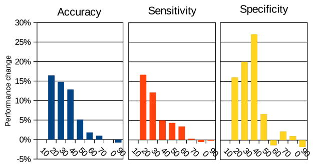
Intra-set whole-rule transfer on the gene expression data [26]. Horizontal axes: proportion of data set used as target. Vertical axis: change in predictive performance compared to training only on the target data. The results are averages of 10 × 5-fold cross-validation.

The amount of transfer (Figure 5) shows similar trends; the measures rr/rl and ar/al are high when the target data set is small, and low when it is large compared to the source data. This is because the source data allows the learning of many good rules, and most of the rules learned on the target data are derived from prior rules. By contrast, the proportion of rules retained out of all prior rules, rr/rp, had a peak around 50%. This means that to maximize retention of prior rules the sizes of the source and target should be roughly equal. This observation agrees with expectation bcause at one extreme, when the target data is large, the source data is very small and the learned rules are not accurate; few rules are learned and even fewer are retained during transfer, leading to a small fraction rr/rp. At the other extreme, when the target data set is very small, it is insufficient for evaluating the learned prior rules accurately; thus again few rules are retained. We also examined the sizes of the antecedents of the learned rules (not shown). In this experimental setup, all rules had one conjunct in their antecedents.

Figure 5.

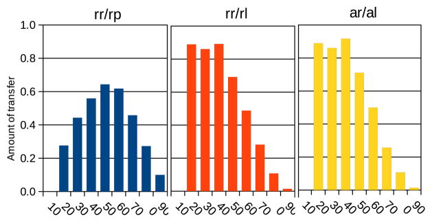
Intra-set whole-rule transfer on the gene expression data [26]. Horizontal axes: proportion of data set used as target. Vertical axis: amount of information retained during transfer learning; rr/rp: number of rules retained as a proportion of prior rules; rr/rl: number of rules retained as a proportion of rules in the new model; ar/al: number of variables in the retained rules, as a proportion of all the variables in the new model. The results are averages of 10 × 5-fold cross-validation.

2.8. Comparison of the Transfer Methods

Using the target data alone performed better than the union of the data sets, so we use it as the baseline. Figures 6 and 7(a) compare the performance of all 4 variants of transfer rule learning. The results in each figure are averaged over 10-fold cross-validation for each experimental setting. The final learned (non cross-validation) rules had at most 4 conjuncts in their antecedents (not shown in the diagrams).

Figure 6.

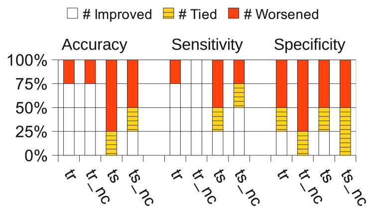
Number of improvements, ties and decreases in performance compared to training on the target data set alone. The results are averages over 10-fold cross-validation over the four protein profiling data sets.

Figure 7.

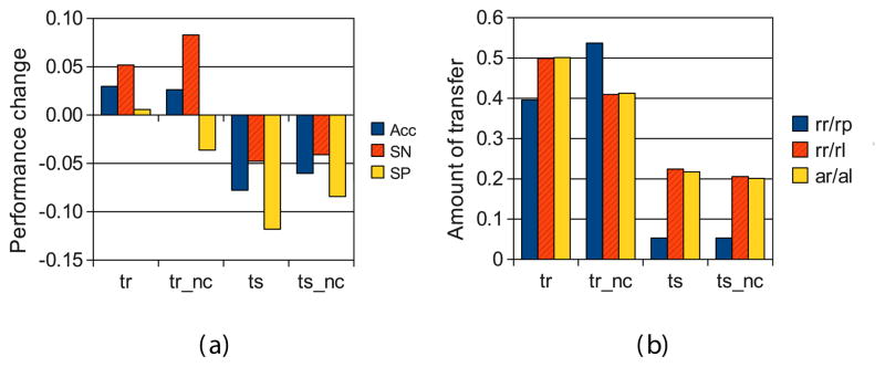
Inter-set transfer with the four variations of the algorithm (horizontal axes). (a) Mean change in predictive performance compared to training on the target data alone. (b) Mean amount of information retained during transfer learning; rr/rp, rr/rl and ar/al have the same meaning as in Figure 5. The results are averages of the two pairs of protein profiling lung cancer data sets, using each data set once as target data in turn and the other one as source, and 10-fold cross-validation over the target data.

Each column of Figure 6 shows the proportion of datasets that each method improved and worsened compared to using the target data alone. We see that the whole-rule transfer methods (“tr” and “tr nc”) improved accuracy in 75% of the cases, while structure transfer methods (“ts” and “ts nc”) only in 0–26% of the cases. Similarly, whole-rule transfer improved sensitivity in 75–100% of the cases, while structure transfer only in 25–50%. Specificity decreased more often than it increased, with all methods.

These trends are visible also in Figure 7(a), which shows the mean changes in performance across all our experiments. Overall, transfer of whole rules performed better than transfer of structures. Moreover, whole-rule transfer with “no coverage” (tr nc) was better on average for sensitivity and accuracy, while the basic rule transfer (tr) was slightly better for specificity. The decrease for structure transfer was due to a dramatic decrease when transferring lung cancer IMAC UPCI to IMAC V and. Without that experiment, the mean performances are markedly greater, and are positive for most measures, though still lower for structure transfer than whole-rule transfer.

That whole-rule transfer performed better than structure transfer is surprising because structure transfer was intended as a way to overcome the difference in discretization between the source data and target data, and thus make prior rules more generalizable on the target data. Recall that structure transfer instantiates the prior rule variables with all possible target data values, and adds all those instantiated rules to the beam for evaluation and further specialization. Thus, this result suggests that the benefit gained from more accurate discretization of the prior rules comes at the cost of adding less accurate rules to the final classifier, which more often than not mis-classify target examples. This could be because the large number of instantiated rules are displacing from the beam other rules that would be more accurate if they survived to be specialized; therefore if the beam was big enough, structure transfer should outperform whole-rule transfer. Another hypothesis is that structure transfer performed poorly because of the way RL learns rules, which is not geared towards learning rule structure (see Section 3).

Another trend in the results is that the no-coverage (“nc”) transfer conditions show a less pronounced change than transfer where prior rules affect the coverage of examples. This is interesting because with the no-coverage condition, prior rules do not interact with other rules via covering during learning. However, rules do interact in this way during inference. Thus, the result suggests that it is beneficial to take account of these coverage interactions between all rules while training, rather than ignore them.

3. Discussion

In this paper, we introduced a simple novel paradigm for transfer learning with interpretable rules. We demonstrated that this method is effective for mass spectrometry and gene expression data, and is particularly helpful when there is a relative abundance of source data compared to target data. In addition to the basic framework, we also demonstrated a novel method to transfer only the rule structure, and this can also be used to transfer knowledge from the literature to a new data set.

An interesting line of future research is to investigate why structure transfer performed poorly. One hypothesis is that structure transfer adds too many instantiated prior rules to the beam and those rules are likely to displace other promising rules whose specializations would have proved more accurate. If the beam is large enough, such rules should not be displaced. To test this hypothesis, we could experiment with a much larger beam. But because a large beam makes the search intractable for practical use, we could also investigate two new transfer methods that avoid unnecessary combinatorial instantiation of variables, yet allow for different distributions between data sets. In particular, both methods would discretize a variable on the source data if this yields the same number of discrete values as discretizing on the target data; only if the number of values differs would we either impose the target data discretization or instantiate the target data values when that variable appears in a prior rule.

Another hypothesis to explain the poor performance of structure transfer is that the way RL learns rules is not geared toward learning structure. We would like to experiment with structure transfer using BRL [17], a rule learner based on RL that uses Bayesian scoring and learns a single rule structure with all possible variable-value instantiations.

It would also be interesting to explore transfer between different types of data, such as between proteomic and genomic data, by creating a mapping between them. Another extension of the algorithm is to allow it to correct errors in variable naming (such as m/z shift in mass spectrometry), by constructing compound variables during the search.

References

- 1.Semmes O, Feng Z, Adam B, Banez L, Bigbee W, Campos D, Cazares L, Chan D, Grizzle W, Izbicka E, et al. Evaluation of serum protein profiling by surface-enhanced laser desorption/ionization time-of-flight mass spectrometry for the detection of prostate cancer: I. Assessment of platform reproducibility. Clinical chemistry. 2005;51(1):102. doi: 10.1373/clinchem.2004.038950. [DOI] [PubMed] [Google Scholar]
- 2.Pelikan R, Bigbee W, Malehorn D, Lyons-Weiler J, Hauskrecht M. Intersession reproducibility of mass spectrometry profiles and its effect on accuracy of multivariate classification models. Bioinformatics. 2007;23(22):3065–3072. doi: 10.1093/bioinformatics/btm415. [DOI] [PubMed] [Google Scholar]
- 3.Caruana R. Multitask learning. Machine Learning. 1997;28(1):41–75. [Google Scholar]
- 4.Pan SJ, Yang Q. Survey on transfer learning. IEEE Transactions on Knowledge Engineering. 2010;22(10):1345–1359. [Google Scholar]
- 5.Blitzer J, McDonald R, Pereira F. Domain Adaptation with Structural Correspondence Learning. Proceedings of the 2006 Conference on Empirical Methods on Natural Language Processing; 2006. pp. 120–128. [Google Scholar]
- 6.Wu P, Dietterich TG. Improving SVM accuracy by training on auxiliary data sources. Proceedings of the 21st International Conference on Machine Learning; Morgan Kaufmann. 2004. pp. 871–878. [Google Scholar]
- 7.Clearwater S, Provost F. RL4: A tool for knowledge-based induction. Proceedings of the 2nd International IEEE Conference on Tools for Artificial Intelligence; 1990. pp. 24–30. [Google Scholar]
- 8.Hennessy D, Gopalakrishnan V, Buchanan BG, Rosenberg JM, Subramanian D. Induction of rules for biological macromolecule crustallization. Proceedings of the International Conference on Intelligent Systems for Molecular Biology; AAAI Press. 1994. pp. 179–187. [PubMed] [Google Scholar]
- 9.Lee YW, Buchanan BG, Mattison DM, Klopman G, Rosenkranz HS. Learning rules to predict rodent carcinogenicity of nongenotoxic chemicals. Mutation Research - Fundamental and Molecular Mechanisms of Mutagenesis. 1995;328(2):127–149. doi: 10.1016/0027-5107(94)00202-g. [DOI] [PubMed] [Google Scholar]
- 10.Lee YW, Buchanan BG, Aronis JM. Knowledge-based learning in exploratory science: learning rules to predict rodent carcinogenicity. Machine Learning. 1998;30(2–3):217–240. [Google Scholar]
- 11.Gopalakrishnan V, Livingston G, Hennessy D, Buchanan BG, Rosenberg JM. Machine-learning techniques for macromolecular crystallization data, Acta Crustallographica. Section D: Biological Crystallography. 2004;60(Pt 10):1705–1716. doi: 10.1107/S090744490401683X. [DOI] [PubMed] [Google Scholar]
- 12.Ryberg H, An J, Darko S, Lustgarten JL, Jaffa M, Gopalakrishnan V, Lacomis D, Cudkowicz M, Bowser R. Discovery and verification of amyotrophic lateral sclerosis biomarkers by proteomics. Muscle and Nerve. 2010;42(1):104–111. doi: 10.1002/mus.21683. [DOI] [PMC free article] [PubMed] [Google Scholar]
- 13.Ranganathan S, Williams E, Ganchev P, et al. Proteomic profiling of cerebrospinal fluid identifies biomarkers for amyotrophic lateral sclerosis. Journal of neurochemistry. 2005;95(5):1461–1471. doi: 10.1111/j.1471-4159.2005.03478.x. [DOI] [PMC free article] [PubMed] [Google Scholar]
- 14.Gopalakrishnan V, Ganchev P, Ranganathan S, Bowser R. Rule learning for disease-specific biomarker discovery from clinical proteomic mass spectra. Data Mining for Biomedical Applications. 2006:93–105. [Google Scholar]
- 15.Lustgarten JL, Visweswaran H, Grover S, Gopalakrishnan V. An evaluation of discretization methods for learning rules from biomedical data sets. Proceedings of the International Conference on Bioinformatics and Computational Biology (BIOCOMP’08); 2008. pp. 527–632. [Google Scholar]
- 16.Kolli VSK, Seth B, Weaver L, Lustgarten JL, Grover H, Gopalakrishnan V, Malehorn D. Maldit of profiling of breast-cancer sera for pattern analysis. Human Proteome Organization (HUPO) Proceedings; 2009. [Google Scholar]
- 17.Gopalakrishnan V, Lustgarten JL, Visweswaran S, Cooper GF. Bayesian rule learning for biomedical data mining. Bioinformatics. 2010;26(5):668. doi: 10.1093/bioinformatics/btq005. [DOI] [PMC free article] [PubMed] [Google Scholar]
- 18.Quinlan JR. C4.5: Programs for Machine Learning. Morgan Kaufmann; San Francisco: 1993. [Google Scholar]
- 19.Breiman L, Friedman J, Olshen R, Stone C. Classification and Regression Trees. Chapman & Hall; 1984. [Google Scholar]
- 20.Provost F, Aronis J, Buchanan B. Tech Rep IS 99-012. Stern School of Business, New York University; 1999. Rule-space search for knowledge-based discovery. [Google Scholar]
- 21.Lustgarten JL. PhD thesis. University of Pittsburgh; 2009. A Bayesian Rule Generation Framework for ‘Omic’ Biomedical Data Analysis. [Google Scholar]
- 22.Fayyad UM, Irani KB. Multi-interval discretization of continuous-valued attributes for classification learning. Proceedings of the Thirteenth International Joint Conference on Artificial Intelligence (IJCKAI-993); 1993. pp. 1022–1027. [Google Scholar]
- 23.Lustgarten J, Gopalakrishnan V, Grover H, Visweswaran S. Improving classification performance with discretization on biomedical datasets. AMIA Annual Symposium Proceedings; 2008; AMIA. 2008. pp. 445–449. [PMC free article] [PubMed] [Google Scholar]
- 24.Yildiz P, Shyr Y, Rahman J, et al. Diagnostic accuracy of MALDI mass spectrometric analysis of unfractionated serum in lung cancer. Journal of Thoracic Oncology. 2007;2(10):893. doi: 10.1097/JTO.0b013e31814b8be7. [DOI] [PMC free article] [PubMed] [Google Scholar]
- 25.Lustgarten JL, Kimmel C, Ryberg H, Hogan W. EPO-KB: a searchable knowledge base of biomarker to protein links. Bioinformatics. 2008;24(11):1418–1419. doi: 10.1093/bioinformatics.btn125. [DOI] [PMC free article] [PubMed] [Google Scholar]
- 26.Golub T, Slonim D, Tamayo P, et al. Molecular classification of cancer: class discovery and class prediction by gene expression monitoring. Science. 1999;286(5439):531. doi: 10.1126/science.286.5439.531. [DOI] [PubMed] [Google Scholar]