A wavelet multiscale denoising algorithm for magnetic resonance (MR) images

Abstract

Based on the Radon transform, a wavelet multiscale denoising method is proposed for MR images. The approach explicitly accounts for the Rician nature of MR data. Based on noise statistics we apply the Radon transform to the original MR images and use the Gaussian noise model to process the MR sinogram image. A translation invariant wavelet transform is employed to decompose the MR ‘sinogram’ into multiscales in order to effectively denoise the images. Based on the nature of Rician noise we estimate noise variance in different scales. For the final denoised sinogram we apply the inverse Radon transform in order to reconstruct the original MR images. Phantom, simulation brain MR images, and human brain MR images were used to validate our method. The experiment results show the superiority of the proposed scheme over the traditional methods. Our method can reduce Rician noise while preserving the key image details and features. The wavelet denoising method can have wide applications in MRI as well as other imaging modalities.

1. Introduction

There is a practical limit on the signal-to-noise ratio (SNR) when acquiring MR image data [1]; post-processing methods to remove noise are important. Normally, denoising methods use the signal averaging principle which is based on the natural spatial pattern redundancy in the images. Gaussian filters have been widely used in many applications such as functional MR imaging (fMRI) [2]. However, they have the disadvantage of blurred edges due to averaging nonsimilar patterns. In order to avoid this problem, many edge-preserving filters have been proposed. One example is an anisotropic diffusion filter (ADF) [3–6]. Such a filter preserves edges by averaging pixels in the orthogonal direction of the local gradient. However, the denoising methods usually erase small features and change image statistics due to their edge enhancement effect.

Another approach for denoising relies on statistical inference of a multiscale representation of images. A prominent example includes methods based on wavelet transforms [7–9]. For denoising MR images, wavelet techniques based on soft thresholding were first applied by Healy [10]. In another approach, a wavelet-based Wiener-filter-like denoising method was used [11] where the magnitude of the MR image was squared and the square of a Rician random variable was modeled by a scaled noncentral chi-square distribution. The prior knowledge of the correlation of wavelet coefficients was used to represent significant features across scales [12]. A wavelet denoising method was compared with Gaussian smoothing methods [13]. A Wiener-like-filtering method was applied in the wavelet domain before the reconstruction of MR images [14]. However, typical wavelet-based methods can produce significant artifacts in the processed images because of the structure of the underlying wavelets.

Other denoising methods include a maximum posteriori estimation technique. Those methods account for Rician noise through a data likelihood term and a spatial smoothing prior [15]. Awate [16] used empirical Bayes for denoising in MRI. The method uses a Markov probability density function (PDF) to estimate the observed corrupted data and thus use it as a prior in the Bayesian. In this way, the Bayesian denoising scheme bootstraps itself by estimating the prior through the optimization of an information theoretic metric using the expectation maximization (EM) algorithm. The parametric filter named non-local means (NLM) for random noise removal is analyzed and adapted to reduce the noise in MR images [17]. Jose [18] proposed a filter to reduce random noise in multi-component MRI by spatially averaging similar pixels using information from all available image components in order to perform the denoising process.

In this paper, a wavelet domain denoising procedure based on the Radon transform is proposed for MR images. The approach explicitly accounts for the Rician nature of the data. We employ the Radon transform to the original MRI data in order to transform it to the Radon domain. This approach is particularly useful to denoise dark regions because of the noise bias in low SNR (dark) regions. Furthermore, a translation invariant wavelet transform is employed to decompose the sinogram into multiscales for denoising step by step. Finally, we apply the inverse Radon transform to reconstruct the original MR images from the denoised sinogram. In the following sections, we describe our methods as well as our results from phantom, simulation brain MRI, and real patient MRI.

2. The distribution of noisy MRI data

One main source of noise in an MRI signal is the thermal noise [19]. The signal component of the measurements is present in both real and imaginary channels; each of the two orthogonal channels is affected by white Gaussian noise [20]. An MR image is usually reconstructed by computing the inverse discrete Fourier transform of the raw data. The noise in the reconstructed complex data is thus complex white Gaussian noise. The magnitude of the reconstructed MR image is used for visual inspection and for automatic computer analysis. Since the magnitude reconstruction is simply the square root of the sum of two independent Gaussian random variables, the magnitude image data are described by a Rician distribution. The term Rician noise is used to refer to the error between the underlying image intensities and the observed data [21]. Rician noise is not zero; meanwhile the mean depends on the local intensity in the image [22].

If the real and imaginary data, with mean values A_R and A_I, respectively, are corrupted by zero mean Gaussian, stationary noise with the standard deviation σ, the probability distribution function of the magnitude data will be a Rician distribution, as described by

$$P_{\text{mag}}(M)=\frac{M}{{\sigma }^2}{\text{e}}^{-(M^2+A^2)/2{\sigma }^2}{I}_0(AM/{\sigma }^2),$$ (1)

where I₀ is the modified Bessel function of the first kind with order zero. The image pixel intensity in the absence of noise is denoted by A, and the measured pixel intensity by M. Here A is given by $A=\sqrt{A_R^2+A_I^2}$. Equation (1) is plotted in figure 1 for different values of the SNR, A/σ. Note that the Rician distribution tends to be a Rayleigh distribution when the SNR goes to zero and approaches a Gaussian distribution at a high SNR. So in low-intensity (dark) regions on an MR image, the Rician distribution tends to be a Rayleigh distribution. In high-intensity (bright) regions, it tends to be a Gaussian distribution. For ratios as small as A/σ = 3 (SNR =10 log₁₀ 3² ≈ 10 dB), it starts to approximate the Gaussian distribution. For a small SNR (A/σ ≤ 1) the Rician distribution is far from a Gaussian distribution. Note that the mean of the distributions, M̄/σ, which is shown by the vertical lines in figure 1, is not the same as A/σ. This bias is due to the nonlinear transform of the noisy data.

Figure 1.

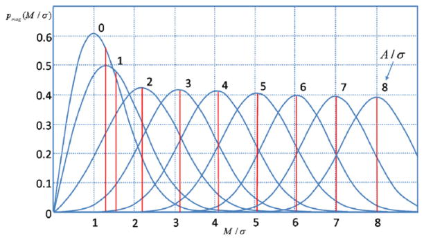
The Rician distribution of M for several SNRs (A/σ) and the corresponding means.

When the SNR is high (A/σ → ∞), an interesting limit of equation (1) is described as

$$\begin{array}{l}{P}_{\text{mag}}(M)\approx \frac{1}{\sqrt{2\pi {\sigma }^2}}{\text{e}}^{-{(M^2-\sqrt{A^2+{\sigma }^2})}^2/2{\sigma }^2}\\ \approx \frac{1}{\sqrt{2\pi {\sigma }^2}}{\text{e}}^{-{(M^2-A)}^2/2{\sigma }^2}.\end{array}$$ (2)

This equation shows that for image regions with high signal intensities the noisy data distribution can be considered as a Gaussian distribution with variance σ² and mean A. Hence, in high SNR regions the noise can be viewed as a Gaussian white noise with variance σ² and zero mean. Based on such an assumption, separation of a signal and noise is fairly straightforward in the wavelet domain. However, the Gaussian approximation may introduce error for regions with a low SNR. As the mean of the magnitude image is not equal to the noise-free image, the magnitude image is biased.

3. Materials and methods

Our method includes four steps. First, we transform the MR image to the Radon domain using the Radon transform. Second, the wavelet transform is employed to decompose sinogram into multiscales. Third, noise variance is evaluated and a thresholding-based method is applied to denoise. Fourth, we reconstruct the denoised sinogram to get the original MRI using the inverse Radon transform.

3.1. Radon transform

The Radon transform of a 2D function is defined as

$$\begin{array}{l}Rf(\alpha ,s)={\int }_{-\infty }^{\infty }{\int }_{-\infty }^{\infty }f(x,y)\delta (s-xcos\alpha -ysin\alpha )\text{d}x\text{d}y\\ \alpha \in [0,\pi ]s\in R,\end{array}$$ (3)

where s is the perpendicular distance of a line from the origin and α is the angle formed by the distance vector. According to the Fourier slice theorem, this transformation is invertible. The Fourier slice theorem states that for a 2D function f (x, y), the 1D Fourier transforms of the Radon transform along s are the 1D radial samples of the 2D Fourier transform of f (x, y) at the corresponding angles [23].

3.2. The distribution of noise in sinogram data

Rician noise differs from Gaussian noise in that it depends on the signal intensity, and the PDF of the noise is very asymmetric for low signal intensities. In brain MR images different regions have different intensities, i.e. white matter (WM), gray matter (GM) and scalp have high intensity, and the noise in these regions is very close to a Gaussian distribution. But other regions such as skull, nasal sinuses and cerebrospinal fluid (CSF) have very low intensity [13], so the noise in these regions is close to a Rayleigh distribution. We sum these regions along a line and thus sum the noise with different distributions. The sum of several Rician distributed noises has a symmetric distribution. Such a sum operation, which is the Radon transform, makes the distribution of noise close to a Gaussian distribution. In figure 2, we compare the sum distribution with the Gaussian distribution with N(μ, σ²). On brain MR images, the low-intensity regions have fewer areas than those with high intensity. For example, the ratio of high-intensity regions to low-intensity regions can be more than 10 along a projection line during the Radon transform. Figure 2 shows the direct comparison between the Gaussian PDF and the sum PDF.

Figure 2.

Gaussian PDF and the PDFs of the sum of two or more Rician distributed sets. In (a)–(d) the sums in sequence are: Sum = P_mag(1) + 10^*P_mag(2), Sum = P_mag(2) + 10^*P_mag(3), Sum = P_mag(3) + 10^*P_mag(4), and Sum = P_mag(1) + 5^*P_mag(2) + 5^*P_mag(3) + 10^*P_mag(4).

In order to measure the similarity degree (R²), we use the following equation:

$$R(x,y)=\text{Cov}(x,y)/[\text{StdDev}(x)·\text{StdDev}(y)],$$ (4)

where Cov is the correlation function and StdDev is the standard variance. This equation is used to measure how well a regression line approximates the real data points statistically, e.g. R² of 1.0 (100%) indicates a perfect fit. From figure 3 we can see that the R² value is close to 1, indicating that the distribution of noisy data is close to a Gaussian function. At the same time we can see that the larger the A/σ the more similar to Gaussian the sum PDF is. In order to demonstrate this conclusion further we calculated an additional 24 sets of the similarity degree (R²) between the real Gaussian PDF and the PDFs of the sum of two or more Rician distributed sets, and it is shown in table 1. In the table we can see that all R²s are over 92%, and all R²s except P_mag(0) + 5^*P_mag(1) and P_mag(0) + 10^*P_mag(1) are over 95%. Here P_mag(0) is the PDF of the magnitude data in the air part inside MR images and not background, because we got rid of noise in the background using a brain mask before the Radon transform. So it is reasonable to use techniques based on the assumption of a Gaussian distribution for sinogram images. In fact, for the heart and brain images, the bright regions in body images have a SNR of over 20 dB (A/σ > 10) [24]. Based on the above-mentioned two facts and equation (2) we demonstrated that the noise in sinogram images is Gaussian noise with mean μ_s and variance ${\sigma }_s^2$. Here from the Radon transform we can obtain μ_s = n_s μ and ${\sigma }_s^2=n_s{\sigma }^2$, and it varies with the number of pixels (n_s) along a line through the MR brain image.

Figure 3.

Correlation plots between the real Gaussian PDF and PDFs of the sum of two or more Rician distributed sets. (a)–(d) are the corresponding correlation plots of (a)–(d) in figure 2, respectively. The horizontal axis is the real Gaussian distribution data and the vertical axis is the distribution sum data.

Table 1.

The similarity degrees (R²s) between the real Gaussian PDF and PDFs of the sum of two or more Rician distributed sets.

Sum	R2	Sum	R2	Sum	R2
Pmag(0) + 5*Pmag(1)	0.9232	Pmag(0) + 5*Pmag(1) + 10*Pmag(2)	0.9509	Pmag(1) + 10*Pmag(4)	0.9902
Pmag(0) + 5*Pmag(2)	0.9556	Pmag(0) + 5*Pmag(2) + 10*Pmag(3)	0.9898	Pmag(1) + 5*Pmag(2) + 10*Pmag(3)	0.9888
Pmag(0) + 5*Pmag(3)	0.9952	Pmag(0) + 5*Pmag(3) + 10*Pmag(4)	0.9845	Pmag(1) + 5*Pmag(3) + 10*Pmag(4)	0.9836
Pmag(0) + 5*Pmag(4)	0.9516	Pmag(0) + 5*Pmag(1) + 5*Pmag(2) + 10*Pmag(3)	0.9590	Pmag(2) + 5*Pmag(3)	0.9964
Pmag(0) + 10*Pmag(1)	0.9235	Pmag(1) + 5*Pmag(2)	0.9541	Pmag(2) + 5*Pmag(4)	0.9750
Pmag(0) + 10*Pmag(2)	0.9596	Pmag(1) + 5*Pmag(3)	0.9953	Pmag(2) + 10*Pmag(4)	0.9956
Pmag(0) + 10*Pmag(3)	0.9971	Pmag(1) + 5*Pmag(4)	0.9501	Pmag(2) + 5*Pmag(3) + 10*Pmag(4)	0.9907
Pmag(0) + 10*Pmag(4)	0.9902	Pmag(1) + 10*Pmag(3)	0.9975	Pmag(3) + 5*Pmag(4)	0.9993

3.3. Wavelet transforms

3.3.1. Wavelet definition

Wavelets are mathematical functions that decompose data into different frequency components that can be studied with a resolution matched to their scale. Wavelet transforms are multiresolution representations of signals and images. They decompose a signal into a hierarchy of scales ranging from the coarsest scale to the finest one. Wavelet coefficients of a signal are the projections of the signal onto the multiresolution subspaces. Wavelets are functions generated from one single function (basis function) called the prototype or mother wavelet by dilations (scalings) and translations (shifts) in the time (frequency) domain. If the mother wavelet is denoted by ψ(t) other wavelets ψ_a,b(t) can be represented as

$${\psi }_{a,b}(t)=1/\sqrt{\mid a\mid }\ast \psi ((t-b)/a),$$ (5)

where a and b are two arbitrary real numbers. The variables a and b represent the parameters for dilations and translations, respectively.

3.3.2. Dyadic discrete wavelet transform

The discrete wavelet transform (DWT) is an implementation of the wavelet transform using a discrete set of the wavelet scales and translation obeying some defined rules. For practical computations, it is necessary to discretize the wavelet transform. The scale parameter a is discretized on a logarithmic grid. The translation parameter b is then discretized with respect to the scale parameter, i.e. sampling is done on the dyadic sampling grid (as the base of the logarithm is usually chosen as 2). The dyadic wavelet transform makes the scale factor binary discrete, while the translation factor maintains continuous change. The discretized scale and translation parameters are given by a = 2^−j and b = k2^−j, respectively, where j, k ∈ Z, the set of all integers. Thus, the family of wavelet functions is represented as

$${\psi }_{j,k}(t)=2^{j/2}\psi (2^{j}t-k).$$ (6)

From the multiresolution point of view, the wavelet decomposition of a discrete time signal x[n] is given by

$$x[n]=\sum _k{c}_{\varphi }(j_0,k){\varphi }_{j_0,k}(n)+\sum _{j=j_0}^{\infty }\sum _k{d}_{\psi }(j,k){\psi }_{j,k}(n),$$ (7)

where ϕ_j0,k, ψ_j,k are the scaling functions and wavelet functions, respectively.

The scaling/approximation and the wavelet/detail coefficients are given respectively as

$$c_{\varphi }(j_0,k)=\sum _{n}x[n]2^{j_0/2}\varphi (2^{j_0}n-k),$$ (8)

$$d_{\psi }(j,k)=\sum _{n}x[n]2^{j/2}\psi (2^{j}n-k),$$ (9)

where j₀ is the starting scale and is always 0. c_ϕ and d_ψ are the scale factor and the wavelet coefficients, respectively, and j is the decomposition level. The development of the fast wavelet transform [25] concludes its identity to two-channel subband decomposition. Thus, it reveals a remarkable relationship between the DWT coefficients of adjacent scales. Using the coefficients d_ψ at a specific level j + 1 we can calculate the coefficients at level j using a filter bank. The wavelet decomposition of a 2D signal can be achieved by applying the 1D wavelet decomposition along the rows and columns of the image separately. This is equivalent to projecting the image onto separable 2D basis functions obtained from the products of 1D basis functions

3.3.3. Translation invariant wavelet

Since the DWT provides good localization in both spatial and spectral domains, low pass filtering is inherent to this transform. The DWT is computationally efficient. The only drawback is that it is not translation invariant, which can introduce artifacts during image reconstruction and exhibit Gibbs phenomena in the neighborhood of discontinuities because of the lack of translation invariance of the wavelet basis. The translation variance in the discrete wavelet transform is due to the required decimation operation (downsampling by two). This problem can be solved by applying additional discrete wavelet decomposition after shifting the sequence by one sample [26]. From the Radon transform we know that the translation along α in the Radon domain corresponds to the rotation of the input image. Although a translation invariant wavelet transform seems to be useful for this application, its application in both directions (s and α) leads to suboptimal results compared with a non-translation invariant wavelet transform. Although the circular shift along α corresponds to the rotation of the image, the circular shift along s does not correspond to a regular geometric distortion. The shift along s in the Radon domain corresponds to an image significantly different from the original image. To solve this problem, we only apply a 1D translation invariant wavelet transform along s [27, 28]. In section 3.5 we will discuss some properties using a 1D wavelet transform along s.

3.3.4. Threshold-based denoising in the wavelet domain

The wavelet coefficients of signals after a wavelet transform contain important information and the wavelet coefficients of noise correspond to smaller amplitude. In our method, a suitable threshold value is selected through different scales, and the wavelet coefficients less than the threshold are set to zero, while retaining the wavelet coefficients greater than the threshold. So the noise signal is effectively inhibited. Finally, the denoised signal is reconstructed using the wavelet inverse transform. It is well known that for independent and identically-distributed Gaussian noise $x\sim N({\mu }_s,{\sigma }_s^2)$ a threshold β = μ_s + σ_s, μ_s + 2σ_s, μ_s + 3σ_s, … will suppress 68.26%, 95.44%, 99.74% of its values. Therefore, we choose β = μ_s + cσ_s, where c is a constant. By taking c between 3 and 4, we can achieve good results. Based on the fact that the variance in each wavelet scale is also ${\sigma }_s^2$ in an orthogonal transformation we can obtain the final threshold

$$\beta ={\mu }_s+c{\sigma }_s=n_s\mu +{cn}_s\sigma .$$ (10)

Under the Gaussian noise assumption, thresholding techniques successfully utilize the unitary transform property of the wavelet decomposition to distinguish statistically the signal components from those of the noise. Our desire, then, is to remove the estimated noise contribution β from each of the wavelet coefficient, and obtain the estimated signal. Although Donoho [29] proved the optimality of soft threshold in theory, Stein threshold has shown better results in SNR improvement. Thus

$$Wf({\widehat{x}}_i)=max(1-{((n_s\mu +{cn}_s\sigma )/\mid Wf(y_i)\mid )}^2,0)Wf(y_i),$$ (11)

where x̂_i is the denoised signal, y_i denotes the noisy observations and Wf (y_i) each of the wavelet coefficients. Finally, we perform the wavelet inverse transform for Wf (x_i) in order to obtain the denoised signal x̂_i.

3.4. Noise mean μ and variance σ² estimation

Our algorithms require the underlying noise variance σ², which is usually unknown and has to be estimated from the data. Typical MR images include an empty region of air outside the patient. A simple estimator is based on the following argument.

From equation (1) we can obtain a special case of the Rician distribution in image regions where only noise is present, A = 0. This is better known as the Rayleigh distribution, and equation (1) reduces to

$$P_{\text{mag}}(M)=\frac{M}{{\sigma }^2}{\text{e}}^{-M^2/2{\sigma }^2}$$ (12)

This Rayleigh distribution governs noise in image regions without signals. The mean for this distribution can be evaluated analytically and is given by

$$\overline{M}=\sigma \sqrt{\pi /2}.$$ (13)

These relations can be used to estimate the ‘true’ noise variance σ² from the magnitude image. So from equation (13) the pixel values in the region outside the patient provide us with a very reliable estimator:

$$\sigma =\sqrt{2}\overline{M}/\sqrt{\pi }\text{and}\mu =\overline{M}.$$ (14)

3.5. Properties of our method

The 1D wavelet transform of an image is equal to the projection of the image onto the 1D basis functions. If we denote the Radon transform of the image by Rf (α, s), the wavelet transform coefficients by Wf (·, ·), and the corresponding 1D orthogonal wavelet basis functions by φ(s), then

$$\begin{array}{l}Wf(·,·)={\int }_0^{\infty }Rf(\alpha ,s)\phi (s)\text{d}s\\ ={\int }_0^{\infty }\left[{\int }_{-\infty }^{\infty }{\int }_{-\infty }^{\infty }f(x,y)\delta (s-xcos\alpha -ysin\alpha )\text{d}x\text{d}y\right]\phi (s)\text{d}s\\ ={\int }_{-\infty }^{\infty }{\int }_{-\infty }^{\infty }f(x,y){\int }_{-\infty }^{\infty }[\delta (s-xcos\alpha -ysin\alpha )\phi (s)\text{d}s]\text{d}x\text{d}y\\ ={\int }_{-\infty }^{\infty }{\int }_{-\infty }^{\infty }f(x,y)\phi (xcos\alpha +ysin\alpha )\text{d}x\text{d}y.\end{array}$$ (15)

By defining h(x, y) = φ(x cos α + y sin α)

$$Wf(·,·)={\int }_{-\infty }^{\infty }{\int }_{-\infty }^{\infty }f(x,y)h(x,y)\text{d}x\text{d}y,$$ (16)

where h(x, y) in 2D is defined from the wavelet function φ(s) in 1D, and it is similar to 2D wavelet transforms except that the point parameter is replaced by a line parameter. The wavelet is a function with scale and point position, while h(x, y) is a function with scale and line position. Hence the wavelet is effective in representing point singularities, and h(x, y) is effective in representing singularities along the line. So our transform can capture singularities along lines and edges in an efficient way.

3.6. Reconstruction

After obtaining the denoised sinogram, we perform the inverse Radon transform in order to obtain the original image. It is defined as

$$f(x,y)={\int }_0^{\pi }R(\alpha ,xcos\alpha +ysin\alpha )\text{d}\alpha ,$$ (17)

where R are the filtered projections. Generally, three different inverse Radon transform methods are the direct inverse Radon transform (DIRT), filtered back-projection (FBP) and convolution filtered back-projection (CFBP) [30]. The DIRT is computationally efficient, but it introduces some artifacts. FBP based on the linear filtering model often exhibits degradation in recovering from noisy data [31]. Spline-convolution filtered back-projection (SCFBP) offers better approximation performance than the conventional lower-degree formulation (e.g. piecewise constant or piecewise linear models) [32]. For SCFBP the denoised sinogram in the Radon domain is approximated in the B-spline space, while the resulting image in the image domain is in the dual-spline space. We used SCFBP to propagate the deniosed sinogram back into the image space along the projection paths.

4. Evaluation and results

Our denoising method has been evaluated by modified brain phantom and simulation brain data. We also applied the method to denoise real brain MR images. We compare with the optimum linear filter, the Wiener filter [33], which is solely adapted to a SNR at a single scale. Meanwhile, a traditional multiscale wavelet method is also applied to these datasets in order to compare with our method. Here Wiener and wavelet methods are used to denoise images in the image domain directly. Finally, in order to prove the efficiency of the proposed method quantitatively an average SNR is used as a quality metric. It is given by

$$\text{SNR}=10{log}_{10}\frac{{\sum }_{j,k}{\mid x[j,k]\mid }^2}{{\sum }_{j,k}{\mid x[j,k]-\widehat{x}[j,k]\mid }^2},$$ (18)

where x[j, k] is the original image x̂[j, k] is the denoised image, with results averaged over all images and reported as mean decibels (dB).

In order to validate our method Rician noise is added to the modified phantom and simulation brain MRI. But while denoising we can get a mask first through a threshold and eliminate the noise outside the phantom and brain. The noise outside the phantom and brain is only used to evaluate the noise variance. The mentioned SNR in the following section only expresses the SNR in the phantom or brain except in outside air. Here for the Wiener filter we used neighborhoods of size 3 × 3 to estimate the local image mean and standard deviation. 2D and 1D db3 wavelets were used in the wavelet filter and our method, respectively, and the images were decompounded into four levels.

4.1. Brain phantom data

Figure 4 illustrates the visual assessment of denoised results on the brain phantom with different noises and the comparison of three methods. In order to compare the denoised effectiveness Rician noise of different degrees is added to this phantom. The images from top to bottom are the phantoms with different degrees of noise, and the images from left to right are the original noised phantom, the denoised result after Wiener, the traditional wavelet and our method in sequence. It can be seen that the Wiener filter makes images a little blurred, and both the traditional wavelet and our method can reduce Rician noise effectively while retaining phantom detail, but our method can suppress Rician noise more.

Figure 4.

Denoised results of brain phantom with different noise using different methods. The first column is the phantom with different degrees of noise. The second column is the results after the Wiener filter. The third column is the results after wavelet. The fourth column is the results after our method.

Figure 5 shows the SNR plots between input SNRs and output SNRs for the three methods. From this figure it can be seen that our method can improve the SNR more than Wiener and the wavelet method. At the same time the output SNR after the Wiener filter grows almost linearly, while the other two methods can improve less with the increase in the input SNR in the original image, and approach the SNR curve of the Wiener filter because the noise is closer to Gaussian noise.

Figure 5.

Input and corresponding output SNR plots for the three methods. The horizontal axis is the input SNR and the vertical axis is the output SNR.

Figure 6 exhibits residuals between the original and denoised phantoms. Comparing these figures we can see that the Wiener filter smoothes the whole image and is uniform for all regions in the image. And the wavelet method performs better for bright regions than dark regions, namely wavelet denoising is better for Gaussian noise than Rician noise under the same condition. The dark part in the phantom is brighter than other parts in the wavelet residual figure. Finally, our method can decrease noise for both dark and bright regions, and its denoised effectiveness in dark regions is better than the other two methods.

Figure 6.

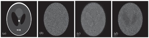
Residuals between the original phantom and denoised phantoms. (a) Original phantom; (b)–(d) the corresponding residuals between the denoised and original phantoms in sequence.

In order to compare the results after different methods quantitatively, we obtain profiles through the original phantom, the denoised phantom, and the phantom after the Wiener filter, the wavelet method and our method as shown in figure 7. The Wiener filter can only smooth a denoised image in the whole image, and in the bright region, the wavelet method and our method have almost the same effect because our method also applies wavelet to denoise. But for dark regions our method performs better than the wavelet method because of the noise distribution. The result after our method is closer to that of the original phantom.

Figure 7.

Comparison of horizontal profiles between the original phantom, noised phantom and phantoms denoised using Wiener, wavelet and our method.

In figure 8 we compare the difference of the denoised effect in the Radon domain. Noised, denoised and no-noise sinograms are shown from left to right in sequence. We obtain a denoised sinogram that is close to the noise-free sinogram visually, and it shows that our method has already decreased the noise in the sinogram.

Figure 8.

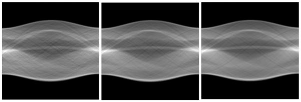
Comparison of the noised (left), denoised (middle) and noise-free (right) sinograms.

4.2. Simulation brain data

We obtained the brain MR images from the McGill phantom brain database for comprehensive validation of the denoising methods. The MR volume contains 181 × 217 × 181 voxels and covers the entire brain. Based on the realistic phantom, an MR simulator is provided to generate specified MR images. The MR tissue contrasts are produced by computing MR signal intensities from a mathematical simulation of the MR imaging physics [34].

As shown in figure 9, the same Rician noise is added to the whole volume and three slices are shown for comparison in this figure. By comparing the dark regions (e.g. skull and CSF) with the bright regions (e.g. WM, GM and scalp) in all denoised images, it can be seen that our method enhances the image contrast and makes the edges clearer than the other two methods. The Wiener method smooths the images and makes whole images blurred. The wavelet method and our method both preserve image details but our method decreases noise more, and this point can be seen from the quantitative SNR. The average SNR of original simulation brain with Rician noise is 17.88 dB, the average SNR after Wiener is 19.33 dB, the average SNR after the wavelet method is 23.12 dB, and the average SNR after our method is 26.84 dB.

Figure 9.

Denoised results of the simulated brain data using different methods. The first column is the noised brain images of different slices. The second column is the results after the Wiener filter. The third column is the results after wavelet. The fourth column is the results after our method.

In the same way we obtain the residuals between the original image and denoised image after different methods as shown in figure 10. As discussed above, the Wiener filter smooths the whole image and its residuals are almost the same except for the edge parts, and the wavelet method is better for bright regions than dark regions, and our method can decrease noise for both dark and bright regions.

Figure 10.

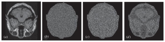
Residuals between the original image and denoised images. (a) Original image; (b)–(d) the corresponding residuals between the denoised and original images in sequence.

In figure 11, we quantitatively compare the profiles through the original image, noised image, and the image after the Wiener filter, wavelet and our method. In this figure, the Wiener filter only smooths the noised image in the whole image and loses the image details. In bright regions, the result after the wavelet method is almost the same as the result after our method, but in dark regions our method excels the wavelet method. We can see the denoised image after our method is closest to the original image and it has the best denoised effect among the three methods.

Figure 11.

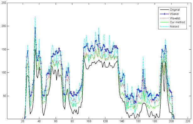
Comparison of horizontal profiles between the original image, noised image and images denoised using Wiener, wavelet and our method.

4.3. Real brain data

The denoising method was also applied to real T1-weighted MR images of human brain. The MR images were acquired with a 4.0 T MedSpec MRI scanner (Bruker BioSpin GmbH, Rheinstetten, Germany) on a Siemens Syngo platform (Siemens Medical Systems, Erlangen, Germany). The T1-weighted magnetization prepared rapid gradient echo sequence (MPRAGE) (TR = 2500 ms and TE = 3.73 ms) was used for the image acquisition. The volume has 256 × 256 × 176 voxels covering the whole brain yielding a 1.0 mm isotropic resolution.

Figure 12 illustrates qualitative comparison of denoised results on T1-weighted MR brain images and the comparison of different methods. We do not perform any preprocessing for the original MR brain image. In this figure our method makes the edges of the MR image clearer and enhances the image contrast. This can be obtained from the property of our method; it can capture singularities along lines and edges in an efficient way. Through comparing the three residuals we can see that the Wiener method makes the whole image smooth and that its residuals are bigger at the edge than in other regions. The traditional wavelet can decrease Rician noise better than Wiener, and it can decrease the noise in dark regions to some degree. In brighter regions with a high SNR, our result shows much less difference from the other two methods, and this means it does not affect the region with little noise. In dark regions that have a low SNR, our result shows bigger difference as compared to the original image than the other two methods, indicating that it greatly decreases the noise. This figure also shows that our method can decrease the noise more than the other two methods, especially for dark regions like skull and CSF (figure 13).

Figure 12.

Qualitative comparison of denoising results obtained with different methods. The first column is the real MR brain image without any processing. From top to bottom, the second column is the denoised results by Wiener, wavelet, and our method, respectively. The third column is the corresponding residuals between the original image and denoised image.

Figure 13.

Qualitative detail comparisons of denoising results obtained with different methods. From left to right: original real image, denoised images and the corresponding residuals. From top to bottom: Weiner, wavelet and our method.

5. Discussion and conclusion

We developed and evaluated a wavelet domain denoising method based on the Radon transform for noise removal in MRI. The new approach explicitly accounts for the Rician nature of the MR data. In high-intensity (bright) regions of the MR images, the Rician distribution is well approximated as Gaussian. In low-intensity (dark) regions, the Gaussian approximation is no longer valid and the Rician distribution has two degrading effects: the random fluctuation of pixel values and the introduction of a signal-dependent bias. Based on the Rician noise encountered in MRI we apply the Radon transform to the original MR image, add Rician noise to MR images to consider the Gaussian distribution for MR sinogram images.

Our method combines the Radon transform and wavelet transform and it can be seen as a translation invariant and orthogonal wavelet transform. Based on the fact that the shifted Radon transform along s corresponds to an image significantly different from the original image, we apply a 1D translation invariant wavelet transform along s. Our method is similar to a 2D wavelet transform except that the point parameters are replaced by the line parameters. The wavelet is a function with scale and point position, while our method is a function with scale and line position. Hence the wavelet is effective in representing point singularities. And our method is effective in representing singularities along the line. So our transform can capture singularities along lines and edges in an efficient way. Based on the nature of noise we show how to obtain accurate thresholds in different scales and evaluate original noise variance.

Our method can not only effectively decrease Rician noise in MRI but also preserve the key image details and features. Brain phantom, a simulation brain MR image and a real brain MR image are used to validate our method. Our method is compared with the optimum linear filter at a single scale, the Wiener filter, and the multiscale traditional wavelet method. Meanwhile, it can enhance the image contrast, and it performs better than the traditional wavelet and Wiener methods in terms of SNR. The experiment results show the superiority of the proposed scheme and outperform the traditional denoising methods. Our denoising method can have wide applications in MR imaging.

References

- 1.Moseley ME, Liu C, Rodriguez S, Brosnan T. Advances in magnetic resonance neuroimaging. Neurol Clin. 2009;27:271–19. doi: 10.1016/j.ncl.2008.09.006. [DOI] [PMC free article] [PubMed] [Google Scholar]
- 2.Petersson KM, Nichols TE, Poline JB, Holmes AP. Statistical limitations in functional neuroimaging: I. Non-inferential methods and statistical models. Phil Trans R Soc B. 1999;354:1239–60. doi: 10.1098/rstb.1999.0477. [DOI] [PMC free article] [PubMed] [Google Scholar]
- 3.Gerig G, Kubler O, Kikinis R, Jolesz FA. Nonlinear anisotropic filtering of MRI data. IEEE Trans Med Imaging. 1992;11:221–32. doi: 10.1109/42.141646. [DOI] [PubMed] [Google Scholar]
- 4.Alexei AS, Chris RJ. Noise-adaptive nonlinear diffusion filtering of MR images with spatially varying noise levels. Magn Reson Med. 2004;52:798–806. doi: 10.1002/mrm.20207. [DOI] [PubMed] [Google Scholar]
- 5.Murase K, Yamazaki Y, Shinohara M, Kawakami K, Kikuchi K, Miki H, Mochizuki T, Ikezoe J. An anisotropic diffusion method for denoising dynamic susceptibility contrast-enhanced magnetic resonance images. Phys Med Biol. 2001;46:2713–23. doi: 10.1088/0031-9155/46/10/313. [DOI] [PubMed] [Google Scholar]
- 6.McGraw T, Vemuri BC, Chen Y, Rao M, Mareci T. DT-MRI denoising and neuronal fiber tracking. Med Image Anal. 2004;8:95–111. doi: 10.1016/j.media.2003.12.001. [DOI] [PubMed] [Google Scholar]
- 7.Delakis I, Hammad O, Kitney RI. Wavelet-based de-noising algorithm for images acquired with parallel magnetic resonance imaging (MRI) Phys Med Biol. 2007;52:3741–51. doi: 10.1088/0031-9155/52/13/006. [DOI] [PubMed] [Google Scholar]
- 8.Weaver JB, Xu YS, Healy DM, Cromwell LD. Filtering noise from images with wavelet transforms. Magn Reson Med. 1991;21:288–95. doi: 10.1002/mrm.1910210213. [DOI] [PubMed] [Google Scholar]
- 9.Yang X, Li P, Zhang X, Bian Z, Wang B. De-noising of the Doppler fetal heart rate signal with wavelet threshold filtering based on spatial correlation. 1st Int. Conf. IEEE on Bioinformatics and Biomedical Engineering, ICBBE 2007; 2007. pp. 928–31. [Google Scholar]
- 10.Healy DM, Weaver JB. Two applications of wavelet transforms in magnetic resonance imaging. IEEE Trans Inf Theory. 1992;38:840–60. [Google Scholar]
- 11.Nowak RD. Wavelet-based Rician noise removal for magnetic resonance imaging. IEEE Trans Image Process. 1999;8:1408–19. doi: 10.1109/83.791966. [DOI] [PubMed] [Google Scholar]
- 12.Pizurica A, Philips W, Lemahieu I, Acheroy M. A versatile wavelet domain noise filtration technique for medical imaging. IEEE Trans Med Imaging. 2003;22:323–31. doi: 10.1109/TMI.2003.809588. [DOI] [PubMed] [Google Scholar]
- 13.Wink AM, Roerdink JBTM. Denoising functional MR images: a comparison of wavelet denoising and Gaussian smoothing. IEEE Trans Med Imaging. 2004;23:374–87. doi: 10.1109/TMI.2004.824234. [DOI] [PubMed] [Google Scholar]
- 14.Wirestam R, Bibic A, Latt J, Brockstedt S, Stahlberg F. Denoising of complex MRI data by wavelet-domain filtering: application to high-b-value diffusion-weighted imaging. Magn Reson Med. 2006;56:1114–20. doi: 10.1002/mrm.21036. [DOI] [PubMed] [Google Scholar]
- 15.Basu S, Fletcher T, Whitaker R. Medical Image Computing and Computer-Assisted Intervention, MICCAI 2006. 2006. Rician noise removal in diffusion tensor MRI; pp. 117–25. [DOI] [PubMed] [Google Scholar]
- 16.Awate SP, Whitaker RT. Feature-preserving MRI denoising: a nonparametric empirical Bayes approach. IEEE Trans Med Imaging. 2007;26:1242–55. doi: 10.1109/TMI.2007.900319. [DOI] [PubMed] [Google Scholar]
- 17.Manjan JV, Carbonell-Caballero J, Lull JJ, Garcia-Marti G, Marti-Bonmati L, Robles M. MRI denoising using Non-Local Means. Med Image Anal. 2008;12:514–23. doi: 10.1016/j.media.2008.02.004. [DOI] [PubMed] [Google Scholar]
- 18.Jose VM, Thacker Neil A, Lull Juan J, Garcia-Marti Gracian. Multicomponent MR image denoising. Int J Biomed Imaging. 2009;2009:897–907. doi: 10.1155/2009/756897. [DOI] [PMC free article] [PubMed] [Google Scholar]
- 19.Macovski A. Noise in MRI. Magn Reson Med. 1996;36:494–7. doi: 10.1002/mrm.1910360327. [DOI] [PubMed] [Google Scholar]
- 20.Anand CS, Sahambi JS. MRI denoising using bilateral filter in redundant wavelet domain. TENCON 2008—IEEE Region 10 Conf; 2008. pp. 1–6. [Google Scholar]
- 21.Gudbjartsson H, Patz S. The Rician distribution of noisy MRI data. Magn Reson Med. 1995;34:910–4. doi: 10.1002/mrm.1910340618. [DOI] [PMC free article] [PubMed] [Google Scholar]
- 22.Sijbers J, Den Dekker AJ, Van Audekerke J, Verhoye M, Van Dyck D. Estimation of the noise in magnitude MR images. Magn Reson Imaging. 1998;16:87–90. doi: 10.1016/s0730-725x(97)00199-9. [DOI] [PubMed] [Google Scholar]
- 23.Jafari-Khouzani K, Soltanian-Zadeh H. Rotation-invariant multiresolution texture analysis using Radon and wavelet transforms. IEEE Trans Image Process. 2005;14:783–95. doi: 10.1109/tip.2005.847302. [DOI] [PMC free article] [PubMed] [Google Scholar]
- 24.Ayres CF. MSc Thesis. University of Minnesota; MN, USA: 2000. A variational approach to MR bias correction. [Google Scholar]
- 25.Mallat SG. A theory for multiresolution signal decomposition—the wavelet representation. IEEE Trans Pattern Anal Mach Intell. 1989;11:674–93. [Google Scholar]
- 26.Pesquet JC, Krim H, Carfantan H. Time-invariant orthonormal wavelet representations. IEEE Trans Signal Process. 1996;44:1964–70. [Google Scholar]
- 27.Jean-Luc S, Candes EJ, Donoho DL. The curvelet transform for image denoising. IEEE Trans Image Process. 2002;11:670–84. doi: 10.1109/TIP.2002.1014998. [DOI] [PubMed] [Google Scholar]
- 28.Do MN, Vetterli M. The finite ridgelet transform for image representation. IEEE Trans Image Process. 2003;12:16–28. doi: 10.1109/TIP.2002.806252. [DOI] [PubMed] [Google Scholar]
- 29.Donoho DL. Denoising by soft-thresholding. IEEE Trans Inf Theory. 1995;41:613–27. [Google Scholar]
- 30.Yazgan B, Paker S, Kartal M. Image reconstruction with diffraction tomography using different inverse Radon transform algorithms. Proc. 1992 Int. Biomedical Engineering Days; 1992. pp. 170–3. [Google Scholar]
- 31.Nam-Yong L, Lucier BJ. Wavelet methods for inverting the Radon transform with noisy data. IEEE Trans Image Process. 2001;10:79–94. doi: 10.1109/83.892445. [DOI] [PubMed] [Google Scholar]
- 32.Horbelt S, Liebling M, Unser M. Discretization of the Radon transform and of its inverse by spline convolutions. IEEE Trans Med Imaging. 2002;21:363–76. doi: 10.1109/TMI.2002.1000260. [DOI] [PubMed] [Google Scholar]
- 33.Skiadopoulos S, Karatrantou A, Korfiatis P, Costaridou L, Vassilakos P, Apostolopoulos D, Panayiotakis G. Evaluating image denoising methods in myocardial perfusion single photon emission computed tomography (SPECT) imaging. Meas Sci Technol. 2009;20:104–23. [Google Scholar]
- 34.Kwan RKS, Evans AC, Pike GB. MRI simulation-based evaluation of image-processing and classification methods. IEEE Trans Med Imaging. 1999;18:1085–97. doi: 10.1109/42.816072. [DOI] [PubMed] [Google Scholar]