

Abstract
Despite the relative recency of its inception, the theory of compressive sampling (aka compressed sensing) (CS) has already revolutionized multiple areas of applied sciences, a particularly important instance of which is medical imaging. Specifically, the theory has provided a different perspective on the important problem of optimal sampling in magnetic resonance imaging (MRI), with an ever-increasing body of works reporting stable and accurate reconstruction of MRI scans from the number of spectral measurements which would have been deemed unacceptably small as recently as five years ago. In this paper, the theory of CS is employed to palliate the problem of long acquisition times, which is known to be a major impediment to the clinical application of high angular resolution diffusion imaging (HARDI). Specifically, we demonstrate that a substantial reduction in data acquisition times is possible through minimization of the number of diffusion encoding gradients required for reliable reconstruction of HARDI scans. The success of such a minimization is primarily due to the availability of spherical ridgelet transformation, which excels in sparsifying HARDI signals. What makes the resulting reconstruction procedure even more accurate is a combination of the sparsity constraints in the diffusion domain with additional constraints imposed on the estimated diffusion field in the spatial domain. Accordingly, the present paper describes an original way to combine the diffusion-and spatial-domain constraints to achieve a maximal reduction in the number of diffusion measurements, while sacrificing little in terms of reconstruction accuracy. Finally, details are provided on an efficient numerical scheme which can be used to solve the aforementioned reconstruction problem by means of standard and readily available estimation tools. The paper is concluded with experimental results which support the practical value of the proposed reconstruction methodology.
Index Terms: Compressed sensing (CS), diffusion magnetic resonance imaging (MRI), high angular resolution diffusion imaging (HARDI), sparse representations, spherical ridgelets, total variation
I. Introduction
Among all contemporary methods of diagnostic medical imaging, magnetic resonance imaging (MRI) is considered to be the modality of choice for diagnosing the majority of neurological and spinal diseases. Central to MRI is the notion of contrast, which is typically defined by the biochemical composition of interrogated tissue as well as by the morphology of its parenchyma. The most prevalent contrast mechanisms used in the current practice are those defined by T1/T2 relaxation times and proton density (PD). Despite their exceptional importance to clinical diagnosis, however, none of the above contrasts allows delineating the morphological structure of the white matter. It is only with the advent of diffusion MRI (dMRI) that scientists have been able to perform quantitative measurements of the diffusivity of white matter, based on which its structural delineation has become possible [1]–[4]. Like any other MRI technique, however, dMRI still remains subject to artifacts and pitfalls [1]. Whereas many of such artifacts can be overcome by means of advanced hardware designs and/or more sophisticated imaging protocols [5], one particularly critical limitation of many dMRI techniques stems from the physics of the acquisition of diffusion MR images, and therefore is impossible to resolve by operational means. Specifically, since collecting the diffusion data requires a repetitive acquisition of MR responses from the same volume of interest for a number of diffusion-encoding gradients, it is the relatively long acquisition times that greatly impair the practical value of this important imaging modality. Accordingly, the practical value of many dMRI methodologies could be improved by shortening the scanning times required for acquisition of diffusion data. A particular method to achieve such an improvement is detailed in this paper.
In the focus of this paper is a specific instance of dMRI known as high angular resolution diffusion imaging (HARDI) [6], [7], which excels in detecting the orientational distribution of water diffusion in the cerebral tissue. In HARDI, it is standard to restrict the diffusion measurements to a single shell in the q-space. In this case, at each spatial location r ∈ ℝ3 within a region-of-interest, its corresponding HARDI signal can be viewed as a real-valued function of the spherical coordinate u ∈
 : = {v ∈ ℝ3|||v||2 = 1}. Moreover, under some general assumptions (see, e.g., [7, Sec. 3.1] for more details), such signals can be modelled according to [6], [7]
| (1) |
where s0 denotes the diffusion signal obtained in the absence of diffusion encoding (i.e., the so-called “b0-image”), αi(r) > 0 are positive weights obeying , b is defined as a function of the shape and amplitude of diffusion-encoding gradients [8, Eq. (3.18)], and are 3×3 diffusion tensors associated with the M(r) neural fibre tracts passing through the r coordinate.
In practical settings, the spherical coordinate u in (1) is sampled at K distinct points . For each uk, its corresponding diffusion-encoded image is measured—the process that results in a total of K scans. On the one hand, increasing K can be expected to provide more information on the measured diffusion system. On the other hand, HARDI scanning times are always limited, which necessitates restriction of K to a reasonably small value. This brings us to the central question addressed in this paper: what is a sufficient number of diffusion-encoding directions to use in HARDI?
It turns out that, under certain assumptions, the above question can be answered in a rigorous manner. Specifically, assuming that each voxel can support only one diffusion flow at most corresponds to setting M(r) = 1 for all r in (1). In this case, at each spatial location, its associated diffusion flow is fully described by a symmetric diffusion tensor D(r), whose estimation is central to diffusion tensor imaging (DTI) [1]–[3], [9]. Since D(r) has only six independent entires, a minimum of if K = 7 diffusion-encoded images are theoretically sufficient to measure s0(r) and recover the values of D(r) by means of, e.g., a least-square fit.1 Unfortunately, the accuracy of DTI is known to deteriorate dramatically at the sites where the neural fibres (or bundles thereof) cross, touch upon each other, or diverge [7], [11]–[14].
As opposed to DTI, HARDI is capable of capturing multimodal diffusion patterns by sampling the unit sphere at a much greater number of orientations (usually between 60 and 100) [6], [11]–[16]. The increase in K makes it possible to describe the diffusion measurements using much more accurate models. Among these are parametric models [17]–[20] which allow HARDI signals to be expressed in terms of a relatively small number of prototype functions. Unfortunately, fitting a parametric model entails minimization of nonconvex cost functionals, which is a noise-sensitive and computationally intensive task, prone to the problem of local minima. The need to predetermine the optimal number of fitting terms is known to be another disadvantage of using the models of this type.
The problems associated with parametric modelling of HARDI signals can be overcome by using nonparametric models, in which case the signals are recovered by projecting the observed data onto properly defined functional subspaces. In particular, the applicability of spherical Fourier analysis to HARDI has been demonstrated in [13], [14], [21], [22], where HARDI signals are approximated by truncated series of spherical harmonics (SH). Despite its stability and computational efficiency, however, the SH-parameterization involves a relatively large number of SHs, which suggests that the latter cannot provide sparse representation of HARDI signals. The main reason for this is rooted in the fact that the energies of elementary signals di(u|r) := exp{−b(uT Di(r)u)} in (1) are concentrated alongside the great circles2 of
, whereas the energy of SHs is spread all over
, and, as a result, a relatively large number of SHs are needed to effectively “encode” di. The inability of the basis of SHs to sparsely represent diffusion signals has led to the proposal of spherical ridgelets in [23], where it was shown that it only takes 6–8 spherical ridgelets on average to represent the HARDI signals with a precision exceeding the precision of their representation using 45 SHs.
The present work takes the ideas of [23] one step further and shows that the availability of a sparsifying basis for HARDI signals can be used to reduce the number of diffusion gradients required for data acquisition. In particular, we suggest to use the theory of compressed sensing (CS) [24], [25] to recover the HARDI signals using the number of spherical samples K in a range of values typical for DTI (i.e., K ∈ [16,24]), thus allowing a multi-fibre analysis of HARDI data to be performed at the “acquisition cost” of a standard DTI.
It is worthwhile noting that the ideas of CS have already paved their way into the field of diffusion imaging [26]–[29]. In this regard, the conceptually closest to the proposed approach is the method reported in [27]. In spite of this similarity, however, there are two principal distinctions which make the present method a more powerful alternative. In particular, the basis functions used in [27] are limited to represent an average dif-fusivity and anisotropy of the white matter, thereby neglecting both intra- and inter-voxel variability of tensors Di(r) in (1). The ridgelet representation, on the other hand, is a multiresolution technique, which possesses an intrinsic ability to deal with a continuum of different diffusion scales. Second, the approach in [27] is applied in a “voxel-by-voxel” manner and it therefore does not take into consideration the spatial regularity of diffusion field. The present paper, on the other hand, proposes a novel formulation of the problem of CS-based reconstruction of diffusion signals, in which the sparsity constraints enforced in the diffusion domain are augmented by regularity constraints enforced in the spatial domain. The resulting reconstruction problem has the format of a convex minimization problem, which is solved using a specially adapted version of the split Bregman algorithm [30], [31]. As will be shown below, the proposed algorithm results in a particularly advantageous computational structure which allows the solution to be computed via a sequence of simple and easily parallelizable steps.
The rest of the paper is organized as follows. Section II provides additional comments on the input-output structure of the proposed algorithm. The construction of spherical ridgelets is briefly outlined in Section III, whereas Section IV gives a formal description of the proposed reconstruction methodology. Some principal details on the numerical implementations of the proposed algorithm are summarized in Section V, with the results of our experimental studies reported in Section VI. Section VII finalizes the paper with a discussion and conclusions.
II. Problem Statement
In the centre of our considerations is the HARDI signal s(u|r) which, when normalized by its related b0-image s0(r), quantifies the attenuation of MR readout caused by the diffusion of water molecules in the direction u ∈
through the spatial position r ∈ ℝ3. In practical settings, both u and r are discretized. Specifically, restricting u to a discrete set of orientations
prescribes the acquisition of diffusion data in the form of K diffusion-encoded images
, with each sk : ℝ3 → ℝ+ corresponding to a given uk. In this case, for a fixed r0, the vector [s1(r0), s2(r0),…, sK(r0)]T ∈ ℝK represents a discretization of s(u|r0). Note that such a discretization follows a linear measurement model, since each sample sk(r0) can be represented as an inner product of s(u|r0) with a Dirac sampling function δuk (u) := δ(1 − u · uk) (where the dot denotes the Euclidean dot product).
Next, given a collection of M spherical ridgelets (defined below), HARDI signals are assumed to be expandable as
| (2) |
with c(r) ∈ ℝM being a vector of spherical ridgelet coefficients which depend on the spatial coordinate r. It is important to note that the set of spherical ridgelets is allowed to be overcomplete, implying
. A practical implication of this fact is that the definition of coefficients c(r) in (2) is, in general, not unique. This nonuniqueness is further aggravated by the fact that c(r) will have to be recovered from an under-sampled set of diffusion measurements, in which case K ≪ M. Overcoming such a severe underdetermination in the problem of estimating the ridgelet coefficients c(r) will be possible based on the fundamental premise of the theory of CS that states that an accurate estimation of c(r) is attainable if the latter is sufficiently sparse and if the sampling and representation bases are sufficiently decorrelated. Whereas the sparsity of c(r) is rooted in the very design of spherical ridgelets [23], the incoherency between the Dirac sampling functions and spherical ridgelets stems from the fact that the former have an infinitely small support, while the support of spherical ridgelets is “smeared” alongside the great circles of
. In particular, in the case of Dirac sampling, the mutual coherence between the Dirac and ridgelet bases is defined as
| (3) |
where ||·||∞ denotes the supremum norm. Straightforward computations show that, for the ridgelet analysis used in the present paper, μ is equal to 0.5659. Since the spherical ridgelets are derived from a set of wavelet functions through the application of the Funk–Radon transform, it is natural to ask what is the value of μ for the corresponding spherical wavelets [32], [33]. It turns out that, for this case, μ would be equal to 2.2925, which is almost five time higher than in the case of ridgelet analysis. Additionally, the mutual coherence of the eighth-order spherical harmonic basis (as used, e.g., in [13]) with respect to the Dirac sampling functions is equal to 1.1631, which is still about two times higher than that of the spherical ridgelets. Thus, this is the relatively low coherence with respect to to the Dirac sampling basis which, in combination with their sparsifying properties, makes the spherical ridgelets an ideal candidate for CS-based reconstruction of HARDI signals. In particular, it will be demonstrated below that it is possible to obtain a faithful reconstruction of HARDI signals using as few as K = 16 diffusion-encoding gradients.
The proposed algorithm produces an estimate of the ridgelet representation coefficients c(r) in (2). Once available, the coefficients provide an access to the analytical definition of diffusion signals by virtue of (2). This can be used in a number of ways. One possibility is to use the coefficients to compute their associated orientation distribution functions [6], based on which a multi-fibre tractography analysis can be performed [34]. Alternatively, (2) could be used to evaluate the diffusion signals over an arbitrarily fine grid of spatial orientations. Such a refined set of “measurements” could be subsequently used to fit a different representation model, whose application to the original data would not have been possible without causing severe underestimation errors. Deconvolving the refined data to estimate the underlying fibre orientation functions [35], [36] would be another important option to follow. In this paper, however, we refrain from questioning which of the above possibilities is more advantageous over the others. Our sole objective here is to specify a signal processing algorithm, which can be used to recover HARDI signals using as small a number K of diffusion-encoded images as possible.
Finally, it should be noted that the primarily purpose of the proposed methodology is to improve the value of HARDI in terms of its time efficiency. Since the improvement is achieved through merely decreasing the number of diffusion-encoding gradients, the proposed method by no means abrogates the use of fast imaging protocols [37], [38] to further accelerate the data acquisition. Furthermore, an additional speed-up can be achieved via applying CS to reconstruct the diffusion encoded images sk from their subcritical samples in the k-space [39]–[41]. Generally speaking, we believe this is a combination of such software and hardware technologies which will eventually lead to substantial improvements in the practical value of HARDI-based diagnosing. In this paper, however, we confine our contribution to showing one particular way of attaining this important objective.
III. Spherical Ridgelets
It is the property of spherical ridgelets to provide sparse representation of diffusion signals in (1) which makes them an unparalleled tool for CS-based reconstruction of HARDI data. To avoid repetitions, in what follows, we present only the most principal points of ridgelets design, while their detailed description can be found in [23].
Spherical ridgelets are constructed using the fundamental principles of wavelet theory [42], [43]. Specifically, let x ∈ ℝ+ and ρ ∈ (0, 1) be a positive scaling parameter. Further, let κ(x) = exp{−ρx(x + 1)} be a Gaussian function, which we subject to a range of dyadic scalings which result in
| (4) |
with j ∈ ℕ := {0, 1, 2, …}. Subsequently, the Gauss–Weier-strass scaling function χj,v :
→ ℝ at resolution j ∈ ℕ and orientation v ∈
is defined as given by [32]
| (5) |
where Pn denotes the Legendre polynomial of order n. It is worth noting that the
 energy of χj,v is concentrated around the spherical point v, with this concentration becoming more and more localized when j approaches infinity.
The spherical ridgelets are designed with the help of the Funk–Radon transform which, for an arbitrary continuous function f:
→ ℝ, is defined as
| (6) |
with σ(v) denoting the great circle perpendicular to direction v, i.e., σ(v):= {u ∈
|u·v = 0}. Subsequently, following [23], the semi-discrete frame
 of spherical ridgelets can be defined as
| (7) |
where the spherical ridgelet functions φj,v are obtained from χj,v according to
| (8) |
with χ−1,v(u) ≡ 0, ∀u ∈
. Using (5), the ridgelets (8) can be redefined in a closed form as (see [44] for details)
| (9) |
where κ−1(n) = 0, ∀n and
| (10) |
Note that the
-norm of φj,v defined in (9) is given by
| (11) |
and, therefore, to make all the spherical ridgelets have a unit norm, they have to be normalized through
| (12) |
The set
in (7) is infinite-dimensional, and hence is not suitable for practical computations. To define a discrete counterpart of
, one has first to restrict the values of the resolution index j to a finite set
| (13) |
where J defines the highest level of “detectable” signal details. Additionally, the set of all possible orientations
v ∈
of spherical ridgelets needs to be discretized as well. To find a proper discretization scheme, we first note that the construction in (9) suggests that the bandwidth of the spherical ridgelets (and therefore the dimensionality of the functional space they belong to) increases proportionally to 2j. Since the space of spherical harmonics of degree n has a dimension of (n + l)2, we define the number of ridgelet orientations at resolution j to be equal to Mj = (2j+1m0 + 1)2, with m0 being the smallest spherical order resulting in κ0(m0) ≤ ε for some predefined 0 < ε ≪ 1 (e.g., ε = 10−6). Consequently, for each j ∈
 , there are a total of Mj ridgelet orientations, which results in a discrete counterpart of
defined as
, there are a total of Mj ridgelet orientations, which results in a discrete counterpart of
defined as
| (14) |
where the subscript d stands for “discrete.” It should be noted that, although the set
 is composed of continuously defined functions, its dimension is finite, since
consists of a total of
spherical ridgelets. To slightly simplify our notation, in what follows, the spherical ridgelets in
will be indexed as φm, with m = 1, 2, …, M being a combined index accounting for both different resolutions and orientations.
is composed of continuously defined functions, its dimension is finite, since
consists of a total of
spherical ridgelets. To slightly simplify our notation, in what follows, the spherical ridgelets in
will be indexed as φm, with m = 1, 2, …, M being a combined index accounting for both different resolutions and orientations.
Given a sampling set of K diffusion-encoding orientations
, one can use (9) to compute the values of the spherical ridgelets in
over this sampling set.3 The resulting values can be stored into a K × M matrix A defined as
| (15) |
Then, for a given vector s(r) := [s(u1|r), s(u2|r),…, s(uK|r)]T ∈ ℝK of the measured values of a diffusion signal, s(u|r) at the spatial location r, the model (2) asserts the existence of representation coefficients c(r) ∈ ℝM such that
| (16) |
where e(r) accounts for both model and measurement noises at location r. Clearly, the non-negligibility of e(r) along with the fact that K ≪ M makes the problem of recovering the representation coefficients c(r) from s(r) a very challenging inverse problem, our solution to which is presented next.
IV. Proposed Reconstruction Framework
A. Composite Regularization of the Ridgelet-Based Reconstruction
Let Ω represent the volume within which diffusion measurements are acquired. Also known as a region of interest, Ω is assumed to be a bounded rectangular subdomain of ℝ3, i.e., Ω := [0, Lx] × [0, Ly] × [0, LZ] ⊂ ℝ3. Let Ωd be a discrete subset of Ω which represents the spatial locations at which the diffusion signal is measured. Specifically, Ωd is assumed to be a uniform lattice which can be formally defined as
| (17) |
where 0 ≤ i < Nx, 0 ≤ j < Ny, and 0 ≤ l < Nz are sampling indices in the direction of x, y, and z coordinates, respectively.
As before, let K and denote the number of diffusion-encoding gradients used for HARDI data acquisition and their associated spatial orientations, respectively. For each uk, HARDI measurements yield a diffusion-encoded image sk, which can be stored and manipulated as an Nx × Ny × Nz array of real numbers, namely sk ∈ ℝNx × Ny × Nz. Alternatively, at a given coordinate r ∈ Ωd, one can combine the values s1(r), s2(r),…, sK(r) into a column vector, s(r) := [s1(r), s2(r),…, sK(r)]T ∈ ℝK (as it was already done in (16)). This vector can then be regarded as a vector of discrete measurements of s(u|r) sampled at orientations . It is worth noting that, according to the above notations, the value sk(r) admits a twofold interpretation, viz. either as the k-th coordinate of vector s(r) or as the value of image sk at spatial position r.
When combined together, the continuum of vectors, s(r) can be regarded as a discrete vector field s: Ω → ℝK, in which case. s(r) has a natural interpretation of the value of s corresponding to position r. The vector space
 of all such vector fields can be endowed with the standard inner product and its related ℓ2-norm defined as
| (18) |
where ||·||2 and ||·||F denote the Euclidean vector and Frobenius matrix norms, respectively.
Another norm on
that we shall make use of is the total variation (TV) semi-norm which is defined as follows. First, let us define the total variation of the kth component sk of the field s (or, equivalently, of the kth diffusion-encoded image sk) in a standard manner as
| (19) |
where
is a three-neighborhood (causal) clique of voxel r. Consequently, the TV norm of the discrete vector field s can be defined in terms of the TV-norms of its K components as [45]
| (20) |
In this paper, we use α = 1.
Now, let
be a set of spherical ridgelets defined by (14), which is assumed to be sufficiently dense to allow each HARDI signal to be expressed according to (2). Analogously to the discrete measurements s(r), the representation coefficients c(r) corresponding to different voxels r can be aggregated into a vector field c ∈
 , where
: Ωd → ℝM (with c(r) being the value of c observed at r). The ℓ1-norm of the elements of
is defined in the standard manner as
, where
: Ωd → ℝM (with c(r) being the value of c observed at r). The ℓ1-norm of the elements of
is defined in the standard manner as
| (21) |
Using the definitions of the vector fields
and
as well as the definition of A in (15), a connection between
and
is established by means of a linear map
 :
→
that is defined as given by
:
→
that is defined as given by
| (22) |
Consequently, using
, the HARDI data formation model can be concisely described by
| (23) |
with e ∈
(||e|| ,2 ≤ ε) accounting for both measurement noise and modelling errors.
The model (23) reduces of the problem of estimation of HARDI signals to the problem of estimation of their corresponding representation coefficients c from the discrete and noisy measurements s. Moreover, since our main intension is to recover the coefficients c using as few diffusion-encoding gradients as possible (implying K ≪ M), there is an infinite number of solutions which would fit the constraint ||
{c} − s||,2 ≤ ε. However, if it is known a priori that, for each r ∈ Ωd, the vector of representation coefficients c(r) is sparse, then a useful estimate of c can be obtained as a solution to the following convex optimization problem [24], [25]
| (24) |
| (25) |
It is important to note that, under the assumption of spatially homogeneous noise e, the problem (24) is separable in the spatial coordinate r. Indeed, due to the way the ℓ2 and ℓ1 norms are defined in (18) and (21), an optimal field c can be recovered by solving for its components
| (26) |
| (27) |
independently at each r ∈ Ωd.
While computationally attractive, the above solution is sub-optimal, since it completely disregards the dependencies which are likely to exist between spatially adjacent HARDI signals. A possible way to take such dependencies into consideration is to require the noise-free version of the measured signal s to possess a minimal TV norm among all possible candidate solutions. This requirement can be translated into the following minimization problem:
| (28) |
where the role of γ > 0 is to balance the relative influence of the sparse and TV terms in the above cost function. The optimization problem (28) can be rewritten in its equivalent Lagrangian form
| (29) |
for some optimal values of λ > 0 and μ > 0 [46].
Below, we are going to specify a particular, computationally efficient method for solving (29). In this connection, it is instructive to outline the following two instances of (29).
B. Sparse-Only Reconstruction
When μ = 0, the functional in (29) becomes separable in the spatial variable r in the sense that, in such a case, an optimal c can be recovered by solving
| (30) |
for each c(r) independently. Note that (30) can be considered to be a Lagrangian form of the optimization problem (26). There exist a broad spectrum of methods which could be used for solution of (30). Some particularly attractive algorithms seem to be those exploiting the principle of iterative shrinkage (IS) (aka iterated thresholding) [47], [48]. The main advantage of such methods consists in their ability to find a solution of (30) through recursive application of a first-order, fixed-point update rule. Specifically, many IS methods take advantage of the update rule given by
| (31) |
where
 {t} = sign(t)(|t| − τ)+ denotes the operator of soft thresholding and ν is chosen to obey ν > ||AAT||. In the present paper, a modification of the iterative update in (31), known as the fast iterative shrinkage thresholding algorithm (FISTA) [49], was employed due to its considerably faster convergence as compared with many alternative “accelerated” methods.
It should be emphasized that, although suboptimal from the viewpoint of spatial-domain regularity, the solution of (30) by means of iterative shrinkage is advantageous for the following practical reasons. First, it suggests a considerable reduction in the data storage, since the thresholding operator
 in (31) sets to zero the representation coefficients with amplitudes less or equal to λ/ν in absolute value. It makes it possible to use sparse data formats to store and manipulate the representation coefficients. Second, the fact that the estimation of c(r) is performed at each voxel independently suggests a natural way to speed up the overall estimation process though parallel computing on a multicore system.
C. TV-Only Reconstruction
When λ = 0, solving the optimization problem (29) is equivalent to simultaneously solving K optimization problems of the form
| (32) |
where k = 0, 1, …, K − 1 and [
{c}]k denotes the kth component of the vector field
{c} ∈
. Let [
{c}]k be denoted by uk, i.e., uk := [
{c}]k. Then, reformulated with respect to uk, the problem (32) can be rewritten as
| (33) |
in which case it can be recognized as the problem of TV-de-noising of the diffusion-encoded image sk [50]. It is important to note that, in contrast to (32), the problem (33) can be solved for each k independently, in which case we say that the estimation becomes separable in the diffusion direction. The current arsenal of methods which can be used for solving (33) is broad [51]–[53]. In the present paper, we employ the algorithm of [54] for the simplicity and elegancy of its implementation as well as for its outstanding convergence properties.
V. Solution Using Split Bregman Algorithm
Directly solving the original problem (29) is difficult because of the compound nature of the regularization it involves. The split Bregman approach [30] allows one to reduce (29) to a simpler form through introduction of an auxiliary variable u ∈
, which can be viewed as a noise-free version of the data field s. Particularly, using u, (29) can be redefined as
| (34) |
Then, starting from an arbitrary p0 ∈
, the Bregman algorithm [55] finds optimal c and u through the following iterations:
| (35) |
for some γ > 0.4 The functional in (35) is supposed to be minimized over two variables, i.e., u and c. However, due to the way the ℓ1 and TV components of this functional have been split, the minimization can now be performed by sequentially minimizing with respect to u and c separately. The resulting iteration steps are
| (36) |
| (37) |
Note that the functional at Step 2 contains two quadratic terms which can be combined together to result in
| (38) |
To yield a substantial reduction in the value of the cost functional in (35), Step 1 and Step 2 should be applied recursively a number of times before the Bregman parameter pt is updated according to (35). It was argued in [56], however, that the extra precision gained through such a repetitive application of Step 1 and Step 2 is likely to be “wasted” when pt is updated. Consequently, it was suggested in [56] to perform these steps only once per iteration cycle. It is interesting to note that, in this case, the split Bregman algorithm transforms into the alternating directions method of multipliers (ADMM) [31], whose convergence is guaranteed by the Eckstein-Bertsekas theorem [57] (see also [31, Theorem 3.1]).
The final algorithm is summarized below. Lines 3–4 of Algorithm 1 correspond to Step 1 in (36), while lines 5–6 correspond to Step 2. An even more important fact to notice is that the optimization problem in line 4 is separable in the spatial coordinate r. This optimization, therefore, can be performed at each voxel independently as discussed in Section IV-B. Moreover, the optimization problem in line 6 is separable in the diffusion coordinate k, and hence it amounts to applying TV-denoising to each of the K components of u independently as discussed in Section IV-C.
Algorithm 1.
ADMM algorithm for sparse-TV reconstruction of HARDI signals
| 1: p ⇐ 0, u ⇐ s |
| 2: while “c keeps changing” do |
| 3: d ⇐ u − p |
| 4: |
| 5: d ⇐ (1 + γ)−1(s + γ(
{c} + p)) |
| 6: |
| 7: p ⇐ p + (
{c} − u) |
| 8: end while |
VI. Results
A. Performance Criteria for Evaluation of Reconstruction Results
Both the choice of diffusion-encoding directions
and of the orientations of spherical ridgelets require the use of a method for discretizing
. Conventional in HARDI are the methods based on the electrostatic repulsion algorithm (aka the Thomson problem). However, since the diffusion signals are symmetric (i.e., s(u|r) = s(−u|r)), it is a unit hemisphere, not the entire
, which actually has to be discretized. In view of the absence of a formulation of the Thomson problem for hemispherical domains, a common practice is to run the standard procedure for twice as many points as needed, followed by keeping only a half of the resulting configuration. However, as the retained points are not explicitly constrained to lie on a hemisphere, they may include nearly antipodal pairs which are likely to introduce undesirable dependencies between the diffusion measurements as well as between the basis functions. This limitation can be overcome by adapting a different sampling strategy. Particularly, in this paper, both the diffusion-encoding directions as well as the orientations of spherical ridgelets have been defined using the method of generalized spiral points [58], in which the sampling points are arranged along a spherical spiral in such a way that the distance between the points along the spiral is approximately equal to the distance between its coils. This method is straightforward to adapt for sampling of the “northern” hemisphere [i.e., {u ∈
|u · [0,0,1]T ≥ 0}], which provides a nearly uniform, unique and analytically computable coverage which is in no respect inferior to the one produced by solving the Thomson problem.
To assess the performance of the proposed algorithm under controllable conditions, experiments with simulated data sets have been performed. In this case, the HARDI signals were generated according to model (1) with different values of M(r), Di(r), and s0(r) = 1, ∀r. The resulting signals were contaminated by variable levels of Rician noise, giving rise to a set of different SNRs. In this work, we adapt the standard definition of the SNR as
| (39) |
where s and s̃ denote an original signal and its noise-contaminated version, respectively, and the norms are computed as defined by (18). It should be noted that, while conventional in the engineering literature in general, the definition (39) is alien to the MRI community, where it is standard to define signal-to-noise ratio as the ratio between the mean magnitude of MR signal and the standard deviation of noise. For the convenience of referencing, when specifying the values of SNR based on (39), its corresponding values in the alternative units will be provided below as well.
In general, the optimal values of parameters λ and μ in (29) should be expected to vary as a function of the noise level. In the present paper, however, no attempts have been extended to optimize these values for different SNRs. Instead, it was found that λ = 0.03 and μ = 0.05 provided acceptable estimation results in all the simulation scenarios, and hence these values have been used throughout the whole study. Following [23], the scaling parameter ρ in (4) was set to 0.5 and the resolution parameter J in (14) was set to be equal to 1, corresponding to a total of three resolution levels. The number of spherical ridgelet orientations were predefined with m0 = 4, resulting in M−1 = 16, M0 = 49, and M1= 169 ridgelets spanning the resolution levels j = −1, j = 0, and j = 1, respectively. Thus, the total number of spherical ridgelets used in the reconstruction was equal to 234.
To quantitatively compare the reconstruction results produced by the proposed and references methods for different numbers of sampling directions K and various SNRs, three performance measures were used. The first of the three was the normalized mean-squared error (NMSE) defined as
| (40) |
with s(r) being a reference HARDI signal corresponding to location r and ŝ(r) being its estimate. Depending on the nature of a specific experiment, the reference signal can be either a simulated signal discretized at 642 spherical points obtained by the third-order tessellation of the icosahedron or a signal reconstructed using a maximum possible number of diffusion-encoding orientations.
One of the most valuable outcomes of HARDI is in providing access to computation of orientation distribution functions (ODFs)—the functions whose modes are likely to coincide with the direction of local diffusion flows [6]. Both the SH-based [22] and ridgelet-based [23] methods of reconstruction of HARDI signals come with analytical expressions which relate the HARDI signals to their corresponding ODFs. The latter can in turn be used to recover the directions of local diffusion flows (or, equivalently, the orientations of their related fibre tracts) using, e.g., the steepest ascent procedure detailed in [23]. Suppose u0 is the true direction of a diffusion flow and ũ is its estimate. Then, the angular orientation error δ can be defined (in degrees) as
| (41) |
In this paper, as a performance measure, we use an average angular orientation error which is obtained by averaging the values of δ computed for all “fibres” within a specified Ωd.
The last performance measure used in this work is the probability Pd of false fibre detection. To define Pd, let M(r) be the true number of fibre tracts passing through voxel r [as defined by model (1)]. Also, let M̂(r) be an estimated number of fibres, which is equal to the number of modes (maxima) of the ODF recovered at position r. Then, one can define
| (42) |
In addition to the quantitative comparison, the reconstruction results will be evaluated through visual comparison as well. In this paper, we choose to visualize spherical functions by means of 3-D surface plots. Such a plot tends to project away from the origin of ℝ3 in the directions along which a spherical function is maximized, while passing near the origin in the directions where the function approaches zero (for a formal definition see, e.g., [59, Def. 1]).
Finally, our choice of reference methods was motivated by the scope of the main statements made in this paper. First, since we argue that the frame of spherical ridgelets is optimally suited for CS-based reconstruction of HARDI signals, its performance has to be compared with that of alternative representation systems. In particular, the basis of spherical harmonics up to the order eight inclusive has been used for a different definition of the sensing matrix A in (15). (Note that, in the case of a real and symmetric analysis, this SH-basis consists of 45 functions.) Additionally, the representation system proposed in [27] has been exploited in the comparative study as well. This system is formed by applying a set of rotations to a Gaussian kernel of the form d(u) = exp{−b(uTD0u)}, with b defined as in (1) and D0 equal to a (diagonal) diffusion tensor having a mean diffusivity of 766 mm2/s and a fractional anisotropy of 0.8. Following [27], the number of rotations (and hence the number of Gaussian basis functions) was set to be equal to 253. For the convenience of referencing, the CS-based reconstruction methods using the spherical ridgelets, the eighth-order spherical harmonics, and the rotated Gaussian kernels will be referred below to as the RDG, SH8, and GSS algorithms, respectively.
To assess the significance of the proposed spatial regularization, all the above algorithms have been applied with two different values of μ in (29), viz. μ = 0 and μ = 0.05. Note that, in the first of these cases, the spatial regularity is ignored, which leads to the sparse-only reconstruction discussed in Section IV-B. In the second case, on the other hand, the spatial regularity is taken into account and the reconstruction is performed by means of the split Bregman algorithm of Section V.
B. Simulation Experiments
To assess the performance of the proposed and reference methods under controllable conditions, two simulated data sets were used. The first set (referred to below as Phantom #1) had a spatial dimension of 12 × 12 pixels, and consisted of two “fibres” crossing each other at the right angle as it is shown in the upper row of subplots of Fig. 1. In addition, each pixel in the set was assigned an extra diffusion flow in the direction perpendicular to the image plane. As a result, the number of diffusion components M(r) in Phantom #1 varied between 1 and 3. Subsequently, model (1) was used to generate corresponding diffusion-encode images for a range of different values of K. Two different values of b, namely b = 1000 s/mm2 and b = 3000 s/mm2 were used for data generation. The diffusion tensors Di(r) in (1) were obtained by applying rotations to a tensor of the form D0 = diag([α, β,β]) where α and β were equal to 1700 · 10−6 mm2/s and 300 · 10−6 mm2/s, respectively. Note that the mean diffusivity and fractional anisotropy of D0 are equal to 766 mm2/s and 0.8, correspondingly. Thus, the same diffusion tensors were used for data synthesis and for the construction of basis functions in the GSS algorithm, thereby allowing the latter to perform under the best possible conditions.
Fig. 1.
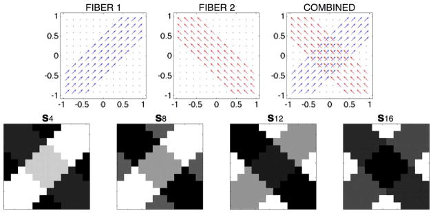
Phantom #1: (Upper row of subplots) The orientations of the individual diffusion flows and their combination. (Lower row of subplots) Examples of the resulting (noise-free) diffusion-encoding images corresponding to four different diffusion-encoding directions.
The lower row of subplots in Fig. 1 depict four examples of diffusion-encoded images obtained for Phantom #1 before their contamination by Rician noise. One can see that the images are piecewise constant functions, which appears to be in a good agreement with the bounded-variation model suggested by (29). However, real images may be more complicated than that. Accordingly, to test the robustness of the proposed regularization scheme, a different simulation phantom was designed. Phantom #2 had a spatial dimension of 16 × 16 pixels and it was obtained through supplementing the configuration of Phantom #1 by an additional circular “fibre” as shown in the upper row of subplots in Fig. 2. The lower row of subplots of the figure show a subset of the resulting diffusion-encoded images, which can be seen to no longer exhibit a piecewise constant behavior characteristic for Phantom #1.
Fig. 2.
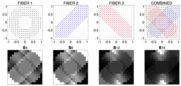
Phantom #2: (Upper row of subplots) The orientations of the individual diffusion flows and their combination. (Lower row of subplots) Examples of the resulting (noise-free) diffusion-encoding images corresponding to four different diffusion-encoding directions.
The simulated diffusion-encoded images were contaminated by three different levels of Rician noise, giving rise to SNR of 24, 18, and 12 dB. (Note that, in the alternative SNR units, the above values correspond to 14.4, 7.2, and 3.6, respectively.) Some typical examples of resulting images are demonstrated in Fig. 3, where the upper row of subplots depict a noise-free version of one of the diffusion-encoded images pertaining to Phantom #1 along with its noise-contaminated counterparts. The lower row of subplots in Fig. 3 depict an analogous set of examples for Phantom #2. Observing the figure, one can see that the SNR values have been chosen so as to cover a range of possible noise scenarios, which could be characterized as moderate-to-severe contamination.
Fig. 3.
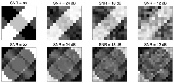
(Upper row of subplots) Diffusion-encoding images of Phantom #1 corresponding to and SNR = ∞, 24, 18, and 12 dB. (Lower row of subplots) Diffusion-encoding images of Phantom #2 corresponding to the same u and the same values of SNR.
As it was mentioned earlier, in our simulation study we compared the performance of three different representation bases, i.e., spherical harmonics (SH8), Gaussian kernels (GSS), and spherical ridgelets (RDG). All the resulting algorithms have been further subdivided into two different types, depending on whether or not the spatial regularization was engaged. Thus, in the absence of the spatial regularization (corresponding to μ = 0), the reconstruction has been performed on a voxel-by-voxel basis, as detailed in Section IV-B. For the convenience of referencing, the corresponding algorithms will be referred to below as SH8-CS, GSS-CS, and RGD-CS. In the case of μ > 0, the estimation has been carried out using the split Bregman method of Section V. The corresponding algorithms will be referred below as SH8-TV, GSS-TV, and RGD-TV.
The upper subplot of Fig. 4 shows the original field of ODFs of Phantom #1 (corresponding to b = 3000 s/mm2), which have been computed based on Tuch’s approximation [6] (i.e., by applying the Funk-Radon transform to the diffusion signals). At the same time, the middle row of subplots of Fig. 4 show the ODFs recovered by (from left to right) SH8-CS, GSS-CS, and RDG-CS with K = 16 and SNR = 18 dB. One can see that the inability of the SH basis to sparsely represent HARDI signals results in a poor performance of SH8-CS. A better result is obtained with GSS-CS, which uses a basis of rotated Gaussian kernels, and therefore has a potential to represent the HARDI signals in a sparse manner. Unfortunately, the excessive correlation between the Gaussian basis functions adversely affects the ability of this method to withstand the effect of noise. Consequently, the reconstruction obtained using GSS-CS suffers from sizeable errors. The RDG-CS method, on the other hand, provides an estimation result of a much higher quality, albeit some inaccuracies are still noticeable in the central part of the phantom. The reconstruction accuracy improves dramatically when the spatial regularization is “switched on,” as it is demonstrated by the bottom row of subplots in Fig. 4. Specifically, while SH8-TV is still unable to provide a valuable reconstruction, the estimates obtained using GSS-TV and RDG-TV represent correctly the “flow structure” of Phantom #1. Moreover, among the latter two methods, RDG-TV is clearly the best performer, resulting in a close-to-ideal recovery of the original ODFs. The superiority of RDG-TV over the alternative methods is further evident in the results presented by Fig. 5, which depicts the reconstructions obtained for Phantom #2 (with the same values of b, K and SNR as above).
Fig. 4.
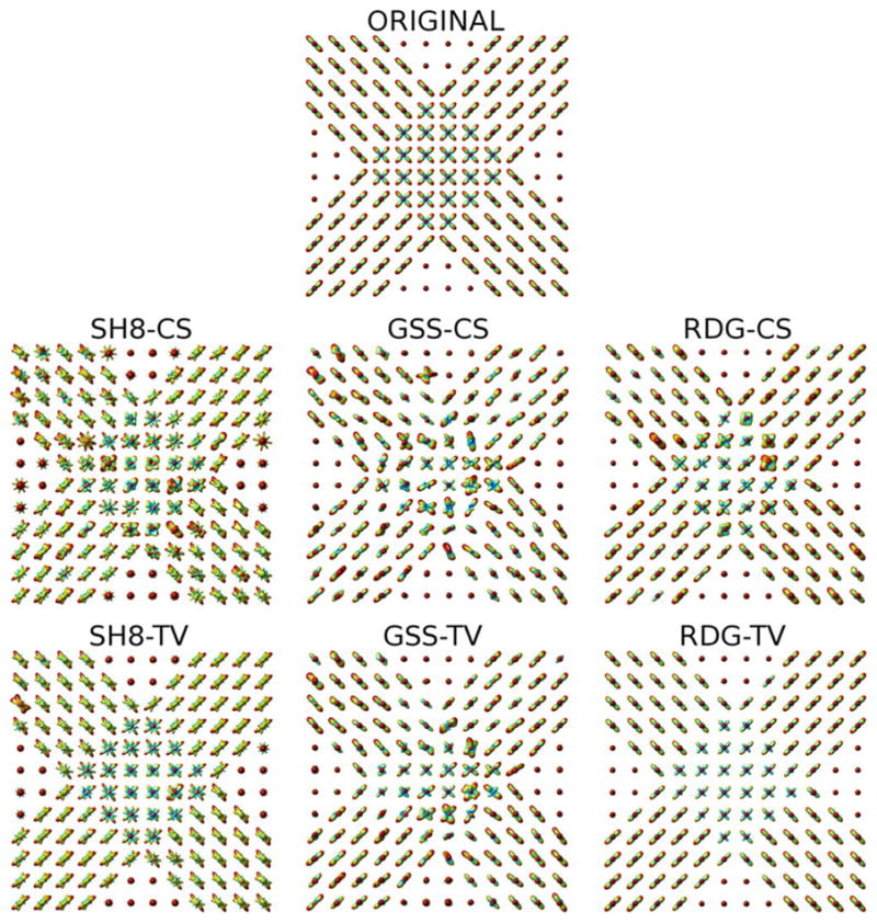
(Upper subplot) Original ODFs of Phantom #1. (Middle row of sub-plots) The ODFs recovered by the SH8-CS, GSS-CS, and RDG-CS algorithms, respectively. (Bottom row of subplots) The ODFs recovered by the SH8-TV, GSS-TV, and RDG-TV algorithms, respectively. The results are shown for the case of K = 16 and SNR = 18 dB.
Fig. 5.

(Upper subplot) Original ODFs of Phantom #2. (Middle row of subplots) The ODFs recovered by the SH8-CS, GSS-CS, and RDG-CS algorithms, respectively. (Bottom row of subplots) The ODFs recovered by the SH8-TV, GSS-TV, and RDG-TV algorithms, respectively. The results are shown for the case of K = 16 and SNR = 18 dB.
In general, the reconstruction results obtained using SH8-CS and SH8-TV have been observed to be of a lower quality in comparison to the other methods under consideration. For this reason, in what follows, only the GSS and RDG methods are compared. Thus, Fig. 6 contrasts the performances of GSS-CS, GSS-TV, RDG-CS, and RDG-TV in terms of the NMSE criterion. One can see that the best performance here is attained by the RDG-TV algorithm, which results in the smallest values of NMSE for both phantoms and for all the tested values of b, SNR, and K. It is also interesting to note that the incorporation of spatial regularization allows GSS-TV to outperform RDG-CS, with the effect of the regularization becoming more pronounced at lower SNRs. On the whole, all the NMSE curves demonstrate an expected behavior, with the error values increasing proportionally with a decrease in SNR, while going down with an increase in the number of diffusion-encoding gradients K. However, as opposed to the others, the NMSE curves obtained with RDG-TV are characterized by a relatively low rate of convergence, which indicates a reduced sensitivity of RDG-TV to the value of K.
Fig. 6.

NMSE as a function of K obtained using the compared methods for different phantoms, SNRs and b-values.
The above algorithms have been also compared in terms of the angular error (41). The results of this comparison are summarized in Fig. 7, which again indicates that the most accurate reconstruction is obtained using the RDG-TV method. As expected, the angular error grows as SNR decreases and converges to a minimum as K increases. As opposed to the case of NMSE, however, there is an additional dependency of the angular error on the type of a phantom in use as well as on the b-value. In particular, the errors obtained for Phantom #2 are (on average) greater than those obtained for Phantom #1. This discrepancy is rooted in the fact that Phantom #2 has a more complex “fibre structure” as compared to Phantom #1. In particular, while the “fibers” of Phantom #1 are designed to cross each other at the right angle, the “fibres” of Phantom #2 are allowed to decussate at much smaller angles, which makes them much harder to resolve. Moreover, this effect becomes more noticeable with a decrease in the b-value, which reduces the resolution of q-ball imaging. Finally, we notice that, on average, GSS-TV performs better than RDG-CS (though still worse than RDG-TV), which justifies the value of spatial regularization.
Fig. 7.

Average angular error δ as a function of K obtained using the compared methods for different phantoms, SNRs and b-values.
The comparison in terms of the rate of false fibre detection Pd (42) was last in the line of our simulation performance tests; its results are shown in Fig. 8. One can see that, in the case of Phantom #1, RDG-TV yields a virtually zero false detection rate for both values of b, whereas the other methods result in considerably higher values of Pd (mainly due to the detection of spurious local maxima in the estimated ODFs). The situation is different for Phantom #2, where all the compared methods yield sizeable errors (especially for b = 1000 s/mm2). However, in comparative terms, the most accurate reconstruction is still obtained by means of the proposed RDG-TV algorithm.
Fig. 8.

The rate of false fibre detection Pd as a function of K obtained using the compared methods for different phantoms, SNRs and b-values.
C. In Vivo Results
As the next validation step, experiments with real HARDI data were carried out. The proposed algorithm was tested on human brain scans acquired on a 3T GE system using an echo planar imaging (EPI) diffusion-weighted image sequence. A double echo option was used to suppress eddy-current related distortions. To improve the spatial resolution of EPI, an eight channel coil was used to perform parallel imaging by means of the ASSET technique with a speed-up factor of 2. The data were acquired using 51 gradient directions (quasi-uniformly distributed over the northern hemisphere) with b = 1000 s/mm2. In addition, eight baseline (b0) scans were acquired, averaged and used for normalization. The following scanning parameters were used: TR = 17000 ms, TE = 78 ms, FOV = 24 cm, 144 × 144 encoding steps, and 1.7 mm slice thickness. All scans had 85 axial slices parallel to the AC-PC line covering the whole brain.
As it was mentioned earlier, using RDG-CS for reconstruction of HARDI signals is advantageous for computational reasons. On the other hand, applying the TV-based regularization has an effect of spatial filtering of the HARDI data. Accordingly, the main question addressed through the in vivo experiments has been whether or not it is possible to supersede the spatial regularization by pre-filtering of HARDI signals. To this end, the RDG-CS algorithm was applied first to the HARDI data containing the full set of K = 51 diffusion gradients. (Note that such dense reconstruction is analogous to the one reported in [23], where the latter is shown to outperform the SH-based estimation [22].) The resulting ODFs have been used as a fiducial against which different reconstruction results were compared.
As the next step, three different subsets of 16, 24, and 32 spherical points were composed out of the original set of 51 diffusion gradients. Within each of these subsets, their corresponding points were chosen so as to result in a quasi-uniform coverage of the northern hemisphere. Accordingly, the HARDI data were rearranged into three data sets of size 144 × 144 × 85 × 16, 144 × 144 × 85 × 24, and 144 × 144 × 85 × 32 to emulate compressed sensing data acquisition. The above sets were used to assess the performance of different reconstruction methods.
Unfortunately, we have not succeeded to find conditions under which the SH8 and GSS algorithms would provide stable reconstruction results (either with or without pre-filtering). The reasons for this fact are easy to discern. First, as it was already noted earlier, the SH8 algorithm uses spherical harmonics which are not suitable for CS-based reconstruction, since they do not provide sparse representation of HARDI signals. Consequently, the reconstructions produced by SH8 are prone to sizable distortions—the result which has already been observed in the computer simulation study. Second, the GSS method is based on a “single resolution” model, in which the bandwidth of the generating Gaussian kernel is matched to the mean diffusivity of the white matter. The local diffusivities of the white matter, however, can deviate substantially from their mean value, with the effect of this deviation exacerbating the overall level of noise. On the other hand, the set of rotated Gaussian kernels is extremely redundant and highly correlated, which adversely affects the restricted isometry property of sensing matrix A [24]. As a result, the GSS-based reconstruction becomes unstable for the values of K used in this study. Accordingly, for the reasons detailed above, only the RDG-CS and RDG-TV algorithms are compared below.
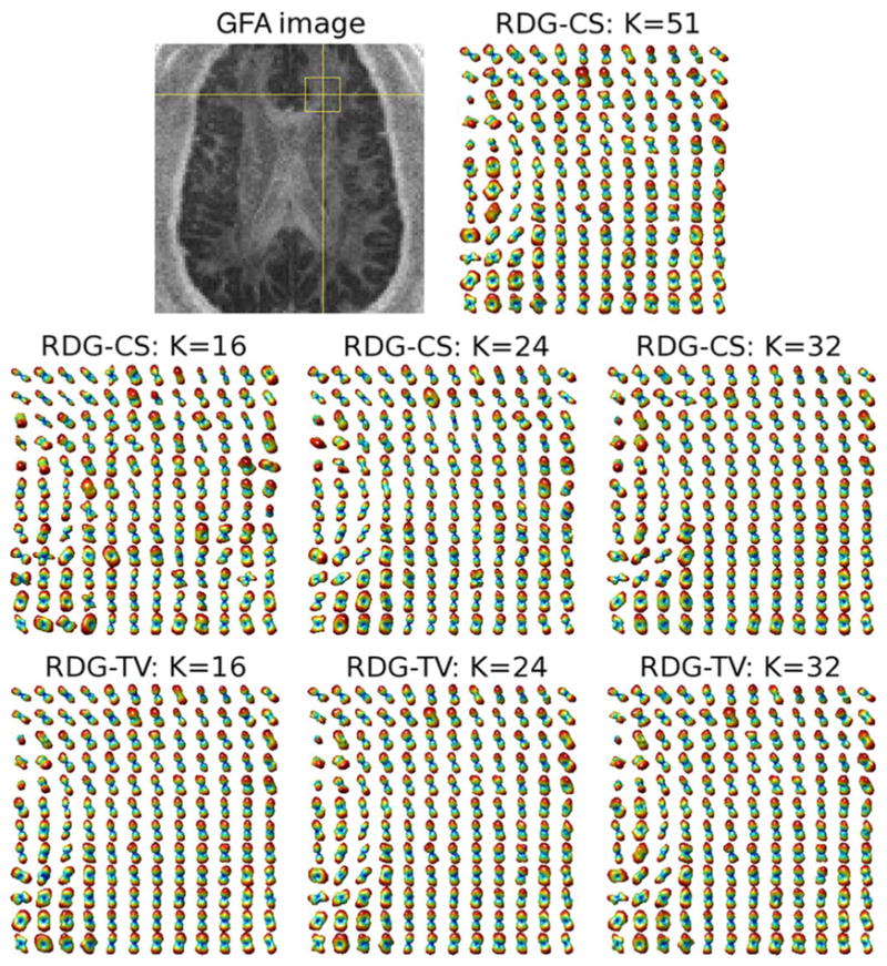
The upper row of subplots in Fig. 9 show the generalized fractional anisotropy (GFA) [6] image of a coronal cross-section of the brain along with the reference field of ODFs corresponding to the region indicated by the yellow rectangular. Anatomically, this region is expected to contain the fibre bundles of corona radiata as well as those of superior longitudinal and arcuate fasciculi. The middle row of subplots in the same figure depict the ODFs reconstructed by RDG-CS using K =16, 24, and 32 diffusion gradients. One can see that the quality of reconstruction progressively improves as K increases. It is important to note that, before applying the RDG-CS algorithm, the diffusion-encoded images had been preprocessed by a TV filter to reduce the effect of measurement noises on the estimation result. However, this preprocessing appears to be not nearly as effective as the spatial regularization of the RDG-TV algorithm, whose reconstruction results are shown in the bottom row of subplots in Fig. 9. The above conclusion is further supported by an additional example of Fig. 10, which shows the reconstructions pertaining to the indicated area within an axial cross-section of the brain. (The relevant fibre bundles here are those of cingulum and corpus callosum). As in the previous example, one can see that the most accurate reconstruction is attained by means of the proposed RDG-TV method. The superiority of RDG-TV is also confirmed by the quantitative figures of Table I, which summarizes the NSME obtained by the compared algorithms for different values of K.
Fig. 9.

(Upper row of subplots) A coronal GFA image and the ODF field of the indicated region recovered by RDG-CS with K = 51. (Middle row of subplots) Estimated ODF fields obtained using RDG-CS with K = 16, K = 24 and K = 32 applied to TV-prefiltered HARDI data. (Bottom row of subplots) Estimated ODF fields obtained using RDG-TV with K = 16, K = 24 and K = 32.
Fig. 10.
(Upper row of subplots) An axial GFA image and the ODF field of the indicated region recovered by RDG-CS with K = 51. (Middle row of subplots) Estimated ODF fields obtained using RDG-CS with K = 16, K = 24 and K = 32 applied to TV-prefiltered HARDI data. (Bottom row of subplots) Estimated ODF fields obtained using RDG-TV with K = 16, K = 24 and K = 32.
TABLE I.
(NMSE ± σ) × 100 Computed Between the Dense and CS-Based Reconstructions Obtained With RDG-CS and RDG-TV
VII. Discussion and Conclusion
When taken all together, the HARDI signals pertaining to a given volume of interest can be described as multi-valued (or, more generally, measure-valued) functions from a subset of ℝ3 to the space of square-integrable spherical functions
(
). Such functions can be thought of as if they had two “modes of variation”—one in the spatial and another in the diffusion domain. Although applying various inverse problems along the spatial and diffusion coordinates independently is not new to the community of medical imaging scientists, formulating a CS reconstruction problem in both domains simultaneously has not been proposed before. Accordingly, the present paper introduced the RDG-TV algorithm which exploits the above idea and can be used for reliable reconstruction of HARDI signals from as few as K = 16 diffusion-encoded scans (as compared to 60–100 scans required by existing reconstruction tools). The algorithm exploits the fact that HARDI signals can be sparsely represented by spherical ridgelets in the diffusion domain, while their associated diffusion-encoded images have bounded variation in the spatial domain. Moreover, it has been shown experimentally that either using different representation bases or excluding the spatial regularization would result in less accurate reconstruction results.
At the practical level, the reconstruction is implemented based on the split Bregman approach (with 20 being the maximum number of Bregman iterations used in this study). The resulting algorithm alternates between two estimation stages (36): first, a sequence of basis pursuit de-noising problems are solved independently on a voxel-by-voxel basis, followed by applying a TV filter to a total of K discrete images. In terms of computational times, applying the FISTA algorithm of [49] to a single voxel with 234 spherical ridgelets, K = 16 and SNR = 18 dB takes MATLAB about 60 ms to complete on a 2.33 GHz Intel Core 2 Duo with a 2 GB SDRAM. At the same time, the TV denoising method of [54] can be executed in about 50 ms on a 128×128 image using the same computational platform. Consequently, depending on the size of a given data set, the proposed RDG-TV method can take from a few to tens of minutes to run in MATLAB. However, the computational times are straightforward to reduce to the scale of seconds by taking advantage of the separable computational structure of RDG-TV, which suggests a considerable speed-up by means of parallel computing. This option constitutes another advantage of the proposed reconstruction algorithm.
In the current paper, the discrete orientations
of diffusion-encoding gradients have been distributed over
in a quasi-uniform manner. Provided that the samples of e(r) in (16) are i.i.d., such a sampling scheme can be shown to be optimal in the MSE sense [60]. It is unclear, however, whether the quasi-uniform sampling remains optimal on the conditions of severe under-sampling (i.e., when K ≪ M) and sparse approximation. In this case, it seems to be theoretically possible to find a better design for
in terms of an optimization of the restricted isometry property [24] of the sensing matrix A in (15). Finding such optimal sampling schemes constitutes a very interesting and important research question, which well deserves an independent and ample treatment.
We believe that the algorithm presented in this paper can be improved in a number of ways. First, the square metric used to assess the model fidelity could be replaced by a different metric, which would be more specific to the nature of Rician noise. Second, the fact that diffusion signals are positive-valued could be explicitly incorporated into the reconstruction process in the form of additional constraints. Lastly, the bounded variation model could be substituted by an alternative model, which could (possibly) provide a better account for the spatial regularity of HARDI signals. Among alternative regularization models are the diffusion-based method of [59], the LMMSE filtering of [61], the weighted least-square regularization approach of [62], and the recent nonlocal mean denoising of [63]. Exploring the above options constitutes essential part of our ongoing research.
Finally, as the experimental study reported in this paper was comparative in its nature, it was not really important what method to use for approximation of ODFs. Specifically, the present results have been obtained using Tuch’s approximation [6]. However, more accurate computation of ODFs is possible based on the solid angle formulation as detailed in [64], [65].5 It should also be noted that the technique proposed in [64] can be applied to multi-shell HARDI data (i.e., the data acquired for a range of b-values). Until recently, collecting such data has been deemed impractical due to extremely long acquisition time required. We believe, however, that the proposed method for CS-based reconstruction of HARDI data has a potential to help multi-shell HARDI develop into a clinically relevant tool of diagnostic imaging.
Acknowledgments
This work was supported by a Discovery grant from NSERC-The Natural Sciences and Engineering Research Council of Canada.
Footnotes
In practice, however, a larger number of gradient directions is employed to reduce the estimation variance, with a typical K being between 25 and 30 [10].
A great circle of
is formed by the intersection of
with a plane passing though it origin. A more formal definition of the great circles is given later in Section III.
Since the definition in (9) involves an infinite summation, the latter needs to be truncated to render the computations practical. In practice, we truncate the summation to index nmax for which the magnitude of the summand drops below 10−9.
Note that the algorithm is guaranteed to converge for any γ > 0. In this work we use γ = 0.5.
We found, however, that the methods in [64], [65] are more sensitive to noise than the one in [6], and this is why we used the latter to avoid inconsistencies in interpreting the estimation results.
Color versions of one or more of the figures in this paper are available online at http://ieeexplore.ieee.org.
Contributor Information
Oleg Michailovich, Email: olegm@uwaterloo.ca, School of Electrical and Computer Engineering, University of Waterloo, ON N2L 3G1, Canada.
Yogesh Rathi, Email: yogesh@bwh.harvard.edu, Psychiatry Neuroimaging Laboratory, Department of Psychiatry, Brigham and Women’s Hospital, Harvard Medical School, Boston, MA 02115 USA.
Sudipto Dolui, Email: sdolui@uwaterloo.ca, School of Electrical and Computer Engineering, University of Waterloo, ON N2L 3G1, Canada.
References
- 1.Bihan DL, Breton E, Lallemand D, Grenier P, Cabanis E, Laval-Jeantet M. MR imaging of intravoxel incoherent motions: Application to diffusion and perfusion in neurological disorders. Radiology. 1986;161:401–407. doi: 10.1148/radiology.161.2.3763909. [DOI] [PubMed] [Google Scholar]
- 2.Basser PJ, Mattiello J, LeBihan D. Estimation of the effective self-diffusion tensor from the NMR spin echo. J Magn Reson Imag, Ser B. 1994;103(3):247–254. doi: 10.1006/jmrb.1994.1037. [DOI] [PubMed] [Google Scholar]
- 3.Mori S, Frederiksen K, Zijl PCMV, Stieltjes B, Kraut MA, Solaiyappan M, Pomper MG. Brain white matter anatomy of tumor patients evaluated with diffusion tensor imaging. Ann Neurol. 2002;51(3):377–380. doi: 10.1002/ana.10137. [DOI] [PubMed] [Google Scholar]
- 4.Johansen-Berg H, Behrens TEJ. Diffusion MRI: From Quantitative Measurements to In-Vivo Neuroanatomy. 1. New York: Academic; 2009. [Google Scholar]
- 5.Rohde GK, Barnett AS, Basser PJ, Marenco S, Pierpaoli C. Comprehensive approach for correction of motion and distortion in diffusion-weighted MRI. Magn Reson Med. 2004;51:103–114. doi: 10.1002/mrm.10677. [DOI] [PubMed] [Google Scholar]
- 6.Tuch DS. Q-ball imaging. Magn Reson Med. 2004;52:1358–1372. doi: 10.1002/mrm.20279. [DOI] [PubMed] [Google Scholar]
- 7.Alexander DC. Multiple-fiber reconstruction algorithms for diffusion MRI. Annals of the New York Academy of Science. 2005;1064:113–133. doi: 10.1196/annals.1340.018. [DOI] [PubMed] [Google Scholar]
- 8.Mori S. Introduction to Diffusion Tensor Imaging. New York: Elsevier; 2007. [Google Scholar]
- 9.Alexander AL, Lee JE, Lazar M, Field AS. Diffusion tensor imaging of the brain. Neurotherapeutics. 2007;4:316–329. doi: 10.1016/j.nurt.2007.05.011. [DOI] [PMC free article] [PubMed] [Google Scholar]
- 10.Jones DK. The effect of gradient sampling schemes on measures derived from diffusion tensor MRI: A Monte Carlo study. Magn Reson Med. 2004;51:807–815. doi: 10.1002/mrm.20033. [DOI] [PubMed] [Google Scholar]
- 11.Tuch DS, Reese TG, Wiegell MR, Makris N, Belliveau JW, Wedeen VJ. High angular resolution diffusion imaging reveals intravoxel white matter fiber heterogeneity. Magn Reson Med. 2002;48:577–582. doi: 10.1002/mrm.10268. [DOI] [PubMed] [Google Scholar]
- 12.Tuch DS, Reese TG, Wiegell MR, Wedeen VJ. Diffusion MRI of complex neural architecture. Neuron. 2003;40:885–895. doi: 10.1016/s0896-6273(03)00758-x. [DOI] [PubMed] [Google Scholar]
- 13.Descoteaux M, Angelino E, Fitzgibbons S, Deriche R. Apparent diffusion coefficients from high angular resolution diffusion images: Estimation and applications. Magn Reson Med. 2006;56(2):395–410. doi: 10.1002/mrm.20948. [DOI] [PubMed] [Google Scholar]
- 14.Hess CP, Mukherjee P, Han ET, Xu D, Vigneron DR. Q-ball reconstruction of multimodal fiber orientations using the spherical harmonic basis. Magn Reson Med. 2006;56:104–117. doi: 10.1002/mrm.20931. [DOI] [PubMed] [Google Scholar]
- 15.Frank L. Anisotropy in high angular resolution diffusion-tensor MRI. Magn Reson Med. 2001;45:935–939. doi: 10.1002/mrm.1125. [DOI] [PubMed] [Google Scholar]
- 16.Wedeen VJ, Hagmann P, Tseng WY, Reese TG, Weisskoff RM. Mapping complex tissue architecture with diffusion spectrum magnetic resonance imaging. Magn Reson Med. 2005;54:1377–1386. doi: 10.1002/mrm.20642. [DOI] [PubMed] [Google Scholar]
- 17.Kreher BW, Schneider JF, Mader I, Martin E, Hennig J, Ilyasov KA. Multi-tensor approach for analysis and tracking of complex fiber configurations. Magn Reson Med. 2005;54:1216–1225. doi: 10.1002/mrm.20670. [DOI] [PubMed] [Google Scholar]
- 18.Banerjee A, Dhillon I, Gosh J, Sra S. Clustering on the unit hyper-sphere using von Mises-Fisher distributions. J Mach Learn Res. 2005;6:1345–1382. [Google Scholar]
- 19.McGraw T, Vemuri B, Yezierski B, Mareci T. Von Mises-Fisher mixture model of the diffusion ODF. presented at the ISBI; Arlington, VA. 2006. [DOI] [PMC free article] [PubMed] [Google Scholar]
- 20.Rathi Y, Michailovich O, Shenton ME, Bouix S. Directional functions for orientation distribution estimation. Med Image Anal. 2009;13(3):432–444. doi: 10.1016/j.media.2009.01.004. [DOI] [PMC free article] [PubMed] [Google Scholar]
- 21.Anderson AW. Measurement of fiber orientation distributions using high angular resolution diffusion imaging. Magn Reson Med. 2005;54:1194–1206. doi: 10.1002/mrm.20667. [DOI] [PubMed] [Google Scholar]
- 22.Descoteaux M, Angelino E, Fitzgibbons S, Deriche R. Regularized, fast, and robust analytical Q-ball imaging. Magn Reson Med. 2007;58:497–510. doi: 10.1002/mrm.21277. [DOI] [PubMed] [Google Scholar]
- 23.Michailovich O, Rathi Y. On approximation of orientation distributions by means of spherical ridgelets. IEEE Trans Image Process. 2010 Feb;19(2):461–477. doi: 10.1109/TIP.2009.2035886. [DOI] [PMC free article] [PubMed] [Google Scholar]
- 24.Candes E, Romberg J, Tao T. Stable signal recovery from incomplete and inaccurate measurements. Commun Pure Appl Math. 2006;59(8):1207–1221. [Google Scholar]
- 25.Donoho D. Compressed sensing. IEEE Trans Inform Theory. 2006;52(4):1289–1306. [Google Scholar]
- 26.Michailovich O, Rathi Y. Fast and accurate reconstruction of HARDI data using compressed sensing. presented at the Med. Image Comput. Computer-Assisted Intervent. (MICCAI); Beijing, China. Sep. 2010; [DOI] [PMC free article] [PubMed] [Google Scholar]
- 27.Landman BA, Wan H, Bogovic JA, Bazin P-L, Prince JL. Resolution of crossing fibers with constrained compressed sensing using traditional Diffusion Tensor MRI. Proc. SPIE,; San Diego, CA. Feb. 2010; [DOI] [PMC free article] [PubMed] [Google Scholar]
- 28.Menzel MI, Khare K, King KF, Tao X, Hardy CJ, Marinelli L. Accelerated diffusion spectrum imaging in the human brain using compressed sensing. presented at the ISMRM; Stockholm, Sweden. 2010. [DOI] [PubMed] [Google Scholar]
- 29.Lee N, Singh M. Compressed sensing based Diffusion Spectrum Imaging. presented at the ISMRM; Stockholm, Sweden. 2010. [Google Scholar]
- 30.Yin W, Osher S, Goldfarb D, Darbon J. Bregman itrative algorithms for ℓ1-minimization with applications to compressed sensing. SIAMJ Imag Sci. 2008;1(1):143–168. [Google Scholar]
- 31.Esser E. Tech Rep CAM Rep 09–31. 2008. Applications of Lagrangian-based alternating direction methods and connections to split Bregman Univ. California Los Angeles. [Google Scholar]
- 32.Freeden W, Schreiner F. Orthogonal and non-orthogonal multiresolution analysis, scale discrete and exact fully discrete wavelet transform on the sphere. Constructive Approximation. 1998;14:493–515. [Google Scholar]
- 33.Kezele I, Descoteaux M, Poupon C, Abrial P, Poupon F, Mangin J-F. Multiresolution decomposition of HARDI and ODF profiles using spherical wavelets. presented at the Workshop Comput. Diffus. MRI, MICCAI; New York. Sep. 2008. [Google Scholar]
- 34.Malcolm J, Shenton M, Rathi Y. Neural tractography using an unscented Kalman filter. Proc IPMI. 2009:126–138. doi: 10.1007/978-3-642-02498-6_11. [DOI] [PMC free article] [PubMed] [Google Scholar]
- 35.Jansons KM, Alexander DC. Persistent angular structure: New insights from diffusion magnetic resonance imaging data. Inverse Problems. 2003;19:1031–1046. [Google Scholar]
- 36.Tournier JD, Calamante F, Gadian DG, Connelly A. Direct estimation of the fiber orientation density function from diffusion-weighted MRI data using spherical deconvolution. NeuroImage. 2004;23:1176–1185. doi: 10.1016/j.neuroimage.2004.07.037. [DOI] [PubMed] [Google Scholar]
- 37.Huang F, Akao J, Vijayakumar S, Duensing GR, Limkeman M. k-t GRAPPA: A k-space implementation for dynamic MRI with high reduction factor. Magn Reson Med. 2005;54(5):1172–1184. doi: 10.1002/mrm.20641. [DOI] [PubMed] [Google Scholar]
- 38.Jung H, Ye JC, Kim EY. Improved k-t BLASK and k-t SENSE using FOCUSS. Phys Med Biol. 2007;52:3201–3226. doi: 10.1088/0031-9155/52/11/018. [DOI] [PubMed] [Google Scholar]
- 39.Lustig M, Donoho D, Pauly JM. Sparse MRI: The application of compressed sensing for rapid MR imaging. Magn Reson Med. 2007;58(6):1182–1195. doi: 10.1002/mrm.21391. [DOI] [PubMed] [Google Scholar]
- 40.Trzasko J, Manduca A, Borisch E. Highly undersampled magnetic resonance image reconstruction via homotopic L0-minimization. IEEE Trans Med Imag. 2009 Jan;28(1):106–121. doi: 10.1109/TMI.2008.927346. [DOI] [PubMed] [Google Scholar]
- 41.Liang D, Liu B, Wang J, Ying L. Accelerating SENSE using compressed sensing. Magn Reson Med. 2009;62:1574–1584. doi: 10.1002/mrm.22161. [DOI] [PubMed] [Google Scholar]
- 42.Daubechies I. Ten Lectures on Wavelets. Philadelphia, PA: SIAM; 1995. [Google Scholar]
- 43.Mallat S. A Wavelet Tour of Signal Processing. 2. New York: Academic; 1999. [Google Scholar]
- 44.Groemer H. Geometric Applications of Fourier Series and Spherical Harmonics. Cambridge, U.K: Cambridge Univ. Press; 1996. [Google Scholar]
- 45.Blomberg P, Chan T. Color TV: Total variation methods for restoration of vector-valued images. IEEE Trans Image Process. 1998 Mar;7(3):304–309. doi: 10.1109/83.661180. [DOI] [PubMed] [Google Scholar]
- 46.Boyd S, Vandenberghe L. Convex Optimization. Cambridge, U.K: Cambridge Univ. Press; 2004. [Google Scholar]
- 47.Daubechies I, Defrise M, DeMol C. An iterative thresholding algorithm for linear inverse problems with a sparsity constraint. Comm Pure Appl Math. 2004;57(11):1413–1457. [Google Scholar]
- 48.Figueiredo MAT, Nowak RD. An EM algorithm for wavelet-based image restoration. IEEE Trans Image Process. 2003 Aug;12(8):906–916. doi: 10.1109/TIP.2003.814255. [DOI] [PubMed] [Google Scholar]
- 49.Beck A, Teboulle M. A fast iterative shrinkage-thresholding algorithm for linear inverse problems. SIAM J Imag Sci. 2009;2(1):183–202. [Google Scholar]
- 50.Rudin LI, Osher S, Fatemi E. Nonlinear total variation based noise removal algorithms. Physica D: Nonlinear Phenomena. 1992;60(1–4):259–268. [Google Scholar]
- 51.Vogel C, Oman M. Iterative methods for total variation de-noising. SIAM J Sci Comput. 1996 Jan;17(1–4):227–238. [Google Scholar]
- 52.Aujol JF. Some first-order algorithms for total variation based image restoration. J Math Imag Vis. 2009;34:307–327. [Google Scholar]
- 53.Osher S, Burger M, Goldfarb D, Xu J, Yin W. An iterative regularization method for total variation-based image restoration. Multi-scale Model Simulat. 2005;4(2):460–489. [Google Scholar]
- 54.Chambolle A, Lions PL. Image recovery via total variation minimization and related problems. Numer Math. 1997;76:167–188. [Google Scholar]
- 55.Bregman LM. A relaxation method for finding a common point of convex sets and its application to the solution of problems in convex programming. USSR Computat Mathematics Mathematical Phys. 1967;(7):200–217. [Google Scholar]
- 56.Goldstein T, Osher S. Tech Rep CAM Report 08-29. 2008. The split Bregman algorithm for L1 regularized problems Univ. California Los Angeles. [Google Scholar]
- 57.Eckstein J, Bertsekas D. Math Programm. 55. 1992. On the Douglas-Rachford splitting method and the proximal point algorithm for maximal monotone operators. [Google Scholar]
- 58.Saff EB, Kuijlaars ABJ. Distributing many points on a sphere. Math Intell. 1997 Dec;19(1):5–11. [Google Scholar]
- 59.Duits R, Franken E. Left-invariant diffusions on the space of positions and orientations and their application to crossing-preserving smoothing of Hardi images. Int J Comput Vis. 2010 doi: 10.1007/s11263-010-0332-z. [DOI] [Google Scholar]
- 60.Dette H, Wiens DP. Robust design for 3-D shape analysis with spherical harmonic descriptors. Statistica Sinica. 2009;19:83–102. [Google Scholar]
- 61.Tristan-Vega A, Aja-Fernandez S. DWI filtering using joint information for DTI and HARDI. Medical Image Anal. 2010;14:205–218. doi: 10.1016/j.media.2009.11.001. [DOI] [PubMed] [Google Scholar]
- 62.Goh A, Lenglet C, Thompson PM, Vidal R. MICCAI. Vol. 5761. New York: Springer; 2009. Estimating orientation distribution functions with probability density constraints and spatial regularity; pp. 877–885. Lecture Notes in Computer Science. [DOI] [PubMed] [Google Scholar]
- 63.Descoteaux M, Wiest-Daessle N, Prima S, Barillot C, De-riche R. MICCAI. New York: Springer; 2008. Impact of Rician adapted non-local means filtering on HARDI. Lecture Notes in Computer Science. [DOI] [PubMed] [Google Scholar]
- 64.Aganj I, Lenglet C, Sapiro G, Yacoub E, Ugurbil K, Harel N. Reconstruction of the orientation distribution function in single- and multiple-shell q-ball imaging within constant solid angle. Magn Reson Med. 2010;64:554–566. doi: 10.1002/mrm.22365. [DOI] [PMC free article] [PubMed] [Google Scholar]
- 65.Tristan-Vega A, Westin CF, Aja-Fernandez S. Estimation of fiber orientation probability density functions in high angular resolution diffusion imaging. NeuroImage. 2009;47:638–650. doi: 10.1016/j.neuroimage.2009.04.049. [DOI] [PubMed] [Google Scholar]