A community participatory study of cardiovascular health and exposure to near-highway air pollution: study design and methods

Abstract

Current literature is insufficient to make causal inferences or establish dose-response relationships for traffic-related ultrafine particles (UFPs) and cardiovascular (CV) health. The Community Assessment of Freeway Exposure and Health (CAFEH) is a cross-sectional study of the relationship between UFP and biomarkers of CV risk. CAFEH uses a community-based participatory research framework that partners university researchers with community groups and residents. Our central hypothesis is that chronic exposure to UFP is associated with changes in biomarkers. The study enrolled more than 700 residents from three near-highway neighborhoods in the Boston metropolitan area in Massachusetts, USA. All participants completed an in-home questionnaire and a subset (440 +) completed an additional supplemental questionnaire and provided biomarkers. Air pollution monitoring was conducted by a mobile laboratory equipped with fast-response instruments, at fixed sites, and inside the homes of selected study participants. We seek to develop improved estimates of UFP exposure by combining spatiotemporal models of ambient UFP with data on participant time-activity and housing characteristics. Exposure estimates will then be compared with biomarker levels to ascertain associations. This article describes our study design and methods and presents preliminary findings from east Somerville, one of the three study communities.

Introduction

Exposure to airborne particulate matter (PM) is linked to increased mortality and morbidity (1 – 4) due largely to cardiovascular (CV) effects (3, 5). Ultrafine particles (aerodynamic diameter <0.1 μm) are a by-product of combustion and comprise approximately 80% – 90% of particle number concentration (PNC) in urban areas (6). Thus, many epidemiology studies use PNC as a surrogate for UFP because size fractionation is often not possible on the scale of monitoring needed for health studies (7). The ability of UFP to penetrate deeply into the lungs combined with their large surface areas appear to cause disproportionately more damage than larger-sized particles per unit mass (5, 8, 9).

Unlike fine PM (PM_2.5 aerodynamic diameter < 2.5 μm), which exhibits relatively uniform concentration distributions in urban areas, UFP tend to exhibit large spatial and temporal variations, particularly near busy roadways (10 – 12). Highways, due to traffic loads and congestion, are important determinants of elevated local concentrations of mobile source pollutants including UFP (10, 13). UFP levels are highest near highways and major roadways and rapidly decrease with distance (10, 11, 13, 14). A recent meta-analysis characterized a spatial gradient for UFP that extended from 100 to 300 m (15). However, gradients of up to 2000 m have been reported, depending on time of day, atmospheric conditions, and local meteorology (14, 16). Elevated UFP levels near roadways may result in an increase in exposure for the estimated 30% – 45% of people in urban areas of the USA who live within 500 m of a highway or major road (17).

Three principal pathways have been proposed to explain the adverse CV effects of inhalation of PM (5). The first pathway begins with pulmonary inflammation, which results in a systemic inflammatory state consisting of oxidative stress, endothelial dysfunction, and accelerated atherosclerosis. Supporting this pathway are observations of associations between PM and markers of systemic inflammation (18, 19). In the second pathway, reflexes in the lung trigger stimulation of the autonomic nervous system causing problems with repolarization and heart rhythms. This pathway is consistent with reports of associations between PM and changes in heart rate variability (20, 21). A third pathway is the direct interaction of PM (or its soluble components) with the CV system resulting in abnormal function (22, 23).

Several epidemiologic studies that used distance to highways and busy roads as proxies for chronic air pollution exposures have reported associations between mortality and CV disease with proximity (24 – 27). Fine PM is an unlikely candidate for near-roadway effects because it shows minimal variation near roadways; UFP, however, are more plausible, due to their spatial distribution. Studies that measured UFP directly have shown acute effects of ambient UFP on biomarkers of CV disease including tumor necrosis factor α receptor II (TNF-RII) (18, 28), interleukin 6 (IL-6) (18, 28, 29), C-reactive protein (CRP) (18, 29), and fibrinogen (30). Other pollutants exhibiting spatial distribution similar to UFP include nitric oxide (NO), carbon monoxide (CO), and, to a somewhat lesser extent, black carbon (BC) and nitrogen dioxide (NO₂). However, toxicologic evidence is stronger for the association of UFP with CV endpoints than for these co-pollutants (31 – 35). Other potentially confounding conditions include sound and socioeconomic status (SES), which may also be associated with distance to highways and major roadways.

The majority of epidemiologic health studies of air pollution exposure have relied on central site measurements, interpolation, or land use regression using central site data to construct ambient annual averages assigned to residential address (36 – 38). These studies probably provide insufficient spatial resolution to accurately assign near-highway exposures. In addition, most studies [with a few exceptions, like the study of Delfino et al. (18, 28)] assume that pollutant levels do not vary significantly between indoors and outdoors and, additionally, that non-residential exposures are uncorrelated with residential exposures. However, accounting for participant time-activity is likely important for accurate exposure assessment, especially for near-highway exposures with substantial geographic variability (39).

The goal of our project is to evaluate the association of near-highway UFP with biomarkers of CV disease in people > 40 years who were not selected on the basis of preexisting illness. Except for Hertel et al. (40), many past studies comprised subjects with CV conditions and may not be generalizable to a broader population. We hypothesize that higher chronic exposure to near-highway UFP will be associated with elevations in biomarkers of inflammation, coagulation, and blood pressure and decreases in ankle brachial pressure index (ABI). We seek to develop accurate estimates of UFP exposure by combining spatiotemporal models of ambient UFP with data on ambient UFP infiltration into homes and information on participant time-activity.

Our approach is innovative in several respects. First, we are modeling near-highway UFP with fine-grain spatial and temporal resolution, something that has not yet been widely reported in the epidemiologic literature. Second, we are assigning individual exposures to near-highway UFP, based on time-activity and other factors. Third, we are using structural equation modeling (SEM) as our primary analytic tool, something that has not been applied widely to the study of ambient PM. Finally, we utilize a community-based participatory research (CBPR) framework in carrying out this research, an approach rare in ambient air pollution studies. This article presents the approach and methods for our study along with preliminary findings from the first of three neighborhoods in which we are working and some early insights into the potential of our approach.

Methods

Study design

The Community Assessment of Freeway Exposure and Health (CAFEH) is a 5-year cross-sectional study of the impact of near-highway air pollution on CV health, specifically blood markers of inflammation, including high-sensitivity CRP (hsCRP), IL-6, TNF-RII, and fibrinogen; brachial blood pressure; and ABI. A diagram showing the key study design elements is presented in Figure 1. The highway of interest is Interstate 93 (I-93), and communities were selected based on distance to the highway, including parts of the cities of Somerville and Malden and the Boston neighborhoods of Chinatown, South Boston, and Dorchester. The communities comprise a wide range of sociodemographics, race/ethnicities, and built environments. We collected human data through the administration of questionnaires, collection of biomarkers from clinical examinations, and laboratory analyses of blood samples. We have extensively monitored UFP and other traffic-related air pollutants, and we are developing an exposure assessment model to test our hypothesis using SEM (41). All participants provided written informed consent; the study was approved by the Institutional Review Board at the Tufts University School of Medicine. Reported here are data from Somerville.

Figure 1.

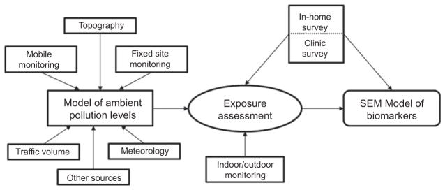
Process diagram of the CAFEH Project.

Community-based participatory research

CAFEH uses a CBPR framework, which combines traditional scientific methods with community engagement. Government agencies, like the NIEHS (National Institute of Environmental Health Science), have integrated CBPR into their models of disease prevention and have created specific funding streams for CBPR initiatives (42). CBPR has been used in the areas of environmental health promotion (43), environmental monitoring (44, 45), and children’s environmental health (46), among others. There is increasing evidence that CBPR can enhance the relevance of research to the community, enrich the quality of data collected, inform findings by incorporating community insight into interpretation, and facilitate translation of results into practice and policy (47, 48).

Details of the CBPR process of CAFEH are published elsewhere (49). Briefly, CAFEH was developed as a direct response to community concerns about air pollution generated from cars and trucks that use I-93 daily. Our community partner, the Somerville Transportation Equity Partnership (STEP), was first formed to advocate for local transportation improvements, including light rail transit and improved walking and bicycling. A related community group, the Mystic View Task Force, working with two Massachusetts firms, Environmental Health & Engineering and Aerodyne Research, conducted preliminary research by monitoring the fate and transport of pollutants from the highway into local residential areas (14). STEP approached Tufts University to conduct a research study of health impacts of near-highway exposures, and the resulting partnership invited similarly impacted groups in Boston to participate.

The CAFEH project includes Tufts University as the lead academic partner, four community partners based within Boston and Somerville (STEP, the Committee for Boston Public Housing, the Chinese Progressive Association, and the Chinatown Residents Association), and researchers at Harvard, Brown, and Boston Universities. Each community partner represents populations living near I-93 in the Boston metropolitan area and brings skills to the project pertaining to public health research, coalition building, recruitment, and education. Community and academic partners are represented in all levels of planning, data collection, and analysis through participation in a steering committee and subcommittees. Community partners were most active during data collection in their neighborhood. An external advisory board of academic institutions, government agencies, health organizations, community members, and elected officials provide input and feedback particularly with regard to policy and practice (49).

Recruitment

The study area for each neighborhood was defined as a 400-m buffer along the highway and an urban background area more than 1000 m from the highway. Our goal was to use highway proximity to recruit a sample that would ultimately have a wide range of UFP exposure levels. One year was spent on data collection in each community. In Somerville, city records were used to create a list of housing units in the study area that were checked via door-to-door enumeration. Each housing unit was linked to a parcel spatial data set obtained from the Harvard Geospatial Library (Harvard University, Cambridge, MA, USA) that included coordinates corresponding to parcel centroids. Recruitment was stratified based on distance to the highway with the goal of increasing exposure contrast. A third of the addresses were drawn from < 100 m (near highway), 100 – 400 m (intermediate highway), and > 1000 m (urban background). A list of random numbers was created in Microsoft Excel (Microsoft, Redmond, WA, USA), which was used to extract the stratified random sample of parcels. The study moved to South Boston/Dorchester in year 2 and Chinatown and Malden in year 3 (details not reported here).

Recognizing the challenges of recruitment, particularly within diverse neighborhoods, we developed a program to increase awareness including the following activities: leafleting all addresses in the study area, obtaining and distributing letters of support from the mayor and/or other local elected officials or prominent community representatives, meeting with community leaders and stakeholders, airing public service announcements on local radio stations, and having articles published in community newspapers and the Boston Globe (50).

We assembled and trained a diverse team of field surveyors to recruit participants and administer the in-home questionnaire, which was available in English, Spanish, Portuguese, Haitian Creole, Chinese (mostly Cantonese, some Mandarin), and Vietnamese. For each target language, we hired two translators who were fully bilingual in English and the target language. The first translator translated from English into the selected language, which was then back-translated by the second, independent translator who was blinded to the original English version to assure accuracy. The majority of the field surveyors lived in the local area. Each surveyor underwent 20 h of training on subject matter and survey techniques followed by field practice. As the study moved from community to community, the composition of the field team changed in terms of age, race/ethnicity, and language to reflect each new community. The field surveyors recruited participants from the random sample by door-knocking. Up to five attempts were made at each address. Eligibility required age > 40 years (because people with greater CV risks have usually been found to have larger responses to PM exposure) and the ability to complete the questionnaire in one of the six languages. When an eligible person agreed to participate, the field surveyors administered the questionnaire in their home or other convenient location. After the completion of the questionnaire, those who agreed to provide biomarker data visited a clinical site within the community. In addition to the random sample, a convenience sample of participants was recruited in each neighborhood to boost numbers. The eligibility for the convenience sample was identical for age and language but required only residence within the study area boundaries. Participants were compensated for completion of the in-home questionnaire and for each clinic visit. In Somerville, the convenience sample included residents of two assisted-living facilities as well as interested residents who contacted CAFEH staff. As a result of these efforts, we enrolled more than 700 residents across the three communities.

Air pollution monitoring

Mobile laboratory

Monitoring was conducted for 12 months in each study area using a mobile platform. Details of data collection, quality assurance, instrument calibration, and data processing methods are provided by Padró-Martínez et al. (51) and are summarized in this article. Mobile monitoring was conducted with the Tufts Air Pollution Laboratory (TAPL), a converted recreational vehicle equipped with fast-response air pollution instruments. A list of the equipment in the TAPL is shown in Table 1. The main pollutant of interest was UFP, measured as the number concentration of particles in the 6- to 3000-nm-size range. In addition, we measured the mass concentration of PM_2.5, NO, nitrogen oxides (NO_x), CO, particle-bound polycyclic aromatic hydrocarbon (pPAH), and BC.

Table 1.

Instrumentation used during environmental monitoring.

Parameter	Equipment	Averaging time
TAPL
UFPa	TSI CPC, Model 3775	1 s
PM2.5	TSI Sidepak, Model AM510	10 s
Particle size distribution	TSI SMPS, Model 3936L75	120 s
NO/NOx	ThermoElectron, chemiluminescence analyzer, Model 42i	20 s
CO	ThermoElectron gas filter correlation analyzer, Model 48i-TLE	10 s
pPAH	Ecochem PAS, Model 2000CE	8 s
BC	Magee Scientific Aethalometer, Model AE-16	60 s
Fixed site (Somerville)
UFPa	TSI CPC, Model 3781	60 s
pPAH	Ecochem PAS, Model 2000CE Ecochem PAS, Model 2000	120 s
Meteorology	Vantage Pro2	5 min

^aPNC is measured as the proxy for UFPs.

Mobile monitoring was performed at different times of the day (high and low traffic periods), days of the week (weekdays and weekends), and seasons (winter, spring, summer, fall). The TAPL was driven at 15 – 40 km/h (9 – 25 mph) along fixed routes that were designed to maximize spatial coverage of the neighborhoods in which the study participants lived. In Somerville, the monitoring route consisted of both the near-highway area < 400 m from the highway (on each side) and the urban background area > 1000 m from the west side of I-93 (note that one third of the study participants lived < 100 m from the highway, another third within 100 – 400 m, and the remainder > 1000 m) (Figure 1). It took ~ 1 h to complete a circuit of the monitoring route; thus, on each monitoring day, five to six circuits were completed. Particle size distribution measurements were also made, but not regularly. Measurements were matched with locations using GPS data collected at 1-s intervals. At the start of each monitoring session, all air pollution instruments and the GPS unit were synchronized by setting the instrument clocks to match the GPS time.

Data processing consisted of several steps. First, measurements associated with instrument errors, as noted in the daily log, were removed. Next, the timestamps for measurements from each instrument were corrected for the time lag between entry of air into the inlet and the time when concentrations were recorded by the instrument. The final step was to remove data that reflected self-sampling of exhaust from the TAPL. Based on our self-sampling decision rules, we removed data if the TAPL speed was < 5 km/h – this usually happened at traffic signals.

Fixed sites

In addition to mobile monitoring, we also collected environmental measurements at fixed sites within each community. In Somerville, two fixed sites were established on either side of the highway (see Figure 2): one was located on the roof of the Mystic Activity Center (MAC) and the other on a ground-level patio at the Blessing of the Bay Boathouse (BBB). Details of data collection, quality assurance, and data processing are provided by Fuller et al. (52). The monitoring equipment at each fixed site was housed in a stainless steel box that contained heating and ventilation to maintain the interior temperature within an appropriate range. Each unit used a water-based condensation particle counter (CPC, Model 3781; TSI, Shoreview, MN, USA) to measure particles in the 6- to 3000-nm-size range as our measure of UFP (Table 1) and a photoelectric aerosol sensor (PAS 2000 or PAS2000CE; EcoChem Analytics, League City, TX, USA) to measure pPAHs. The MAC site also recorded meteorologic variables including wind speed, wind direction, temperature, and relative humidity using a Vantage Pro2 weather station (Davis Instrument, Hayward, CA, USA). UFP was recorded as 1-min averages, pPAHs as 2-min averages, and meteorology as 5-min averages according to the data-storage capacity of each instrument.

Figure 2.

Map of southeast Somerville, MA, USA, showing I-93, roadways, fixed monitoring sites, and approximate locations of study participants.

Residential sites

Residential monitors were placed in 18 homes in Somerville to measure both indoor and outdoor UFP and assess infiltration. Fuller et al. (53) provide the details of residential monitoring in Somerville. Each monitor collected data for 1 – 2 weeks, which consisted of a water-based CPC (Model 3781, TSI) for the measurement of UFP, a PAS (PAS 2000CE; EcoChem Analytics) for measurement of pPAHs, and a HOBO (Onset Computer, Pocasset, MA, USA) for the measurement of temperature and humidity. Each residential monitor contained indoor and outdoor sampling lines of similar length made of stainless steel and flexible conductive Tygon^® tubing (⅜ in. diameter). The indoor line was located on the top of the box and the outdoor line ran through a specially designed window guard and extended ~ 0.5 m from the side of the house. A solenoid valve switched the flow of air between the two lines at approximately 15-min intervals. The monitor was placed in either the living room or the bedroom. The flow rate was held constant at 0.12 L/min, and sampling instruments were checked for adequate flows and functioning before and during each monitoring session.

Human data collection

Survey instruments

Participants completed an in-home questionnaire and supplemental questionnaires during their clinical visits. We describe the questionnaire items below.

Baseline demographics

Each participant provided information on age, sex, education level, relationship status (54), number of people in the household, household income, race/ethnicity, country of birth (55), prior residential location, type of employment, and employment status (55 – 57).

Health status and medications

Participants were asked to self-report whether they had been diagnosed with common CV diseases by a doctor and the year in which they were first diagnosed using questions modified from the Nutrition, Aging, and Memory in Elders project (58). Each participant was asked to show his/her prescribed medications to the interviewing field team member, who in turn recorded the medication name and dosage directly from the label. The supplemental questionnaire, administered at clinic visits, recorded recent acute illnesses (e.g., influenza).

Health behaviors

Participants reported whether they smoked currently or in the past, the amount they smoked, and the duration they had smoked (59 – 61). Physical activity was recorded as light-moderate or vigorous, using questions from the National Center for Health Statistics survey (NCHS) (54). Alcohol consumption was recorded in the supplemental questionnaire including the number of years the participant had consumed alcohol, the amount, frequency, and recent (past 24 h) consumption.

Social factors

Social stress was measured during the in-home questionnaire using a validated 4-item perceived stress scale (62). The supplemental questionnaire included questions on recent life events (e.g., loss of a job) and perceived discrimination (63, 64).

Diet

A set of 15 questions modified from the NCHS survey (54) was included in the in-home questionnaire in which the participant described the type of foods eaten. The supplemental questionnaire included similar questions as well as questions on portion size. The aim of these questions was to group participants into broad dietary categories.

Time-activity

As part of the in-home questionnaire and second clinical visit, participants reported their time-activity for one recent weekday/workday and one recent weekend/non-workday. Participants reported their presence in the following microenvironments for each hour out of the 24-h day: home (inside), home (outside), school/work, or other. Time spent on a highway and use of specific modes of transportation, like walking or subway, were also recorded. We sought highly accurate data on a small number of actual days rather than for “typical” days as has been the approach in another study (61).

Fifteen participants who were part of the residential sampling program also wore GPS receivers during the course of monitoring to track their movements (GPSMap 60Csx; Garmin, Olathe, KS, USA). The receiver was small and lightweight and could be clipped to a belt or purse. Participants in the GPS substudy completed a daily record of locations, including short- and long-distance travel away from their homes, for the duration of monitoring in their home. GPS data were used to validate self-reported time-activity.

Combustion exposures

Questions covering potential exposures to combustion sources were included in both the community and supplemental questionnaires. We asked participants about home heating fuel, location of boilers, and use of space heaters or fireplaces for secondary heating. In the supplemental questionnaire, we asked participants to report recent use of a fireplace, grill, candles or incense, wood- or coal-burning stove, and gasoline- or kerosene-powered equipment. Participants reported if they had cooked with oil, burned trash, or traveled on a highway or busy city streets in the past week. We also recorded if participants had smoked or been in specific locations (e.g., car) with a smoker to understand exposure to direct and environmental tobacco smoke.

Other exposures

The in-home questionnaire included questions on household conditions that might modify exposure to indoor and outdoor pollutants. We included questions concerning the opening of windows and air-conditioning use. Occupational exposure to sources of combustion and chemicals was also recorded in the inhome questionnaire (59– 61).

Biomarker data collection

Participants were asked to provide biomarker data at up to two clinical visits. Venous blood samples were collected, fractionated into plasma, buffy coat, and red blood cells, and frozen at − 80 °C for the analysis of inflammatory markers. The stored samples were analyzed in batches for each neighborhood using immunoassay kits for hsCRP (SPQ High Sensitivity CRP Reagent Set; DiaSorin, Stillwater, MN, USA), fibrinogen (κ-Assay; Kamiya Biomedical, Seattle, WA, USA), TNF-RII (Quantikine; R&D Systems, Minneapolis, MN, USA), and IL-6 (Quantikine HS; R&D Systems). Finger-stick blood samples were analyzed for lipid profile [total cholesterol, low-density lipoprotein (LDL), high-density lipoprotein (HDL), and triglycerides] on site using a CardioChek PA device (Polymer Technology Systems; Indianapolis, IN, USA). Height and weight were collected for the calculation of body mass index using a standard scale (Model 8761321009; SECA, Hamburg, Germany) and stadiometer (Model # 905055; Shorr Productions, Olney, MD, USA), respectively. Systolic and diastolic blood pressures were taken three times using an automatic blood pressure machine (Model HEM711ACN2; Omron Healthcare, Kyoto, Japan) with the participant seated, following a period of rest. The right arm was taken first, followed by the left arm, and then the right arm again. The collection of blood pressure in both arms allows for examination of interarm difference in blood pressure. For the purpose of ABI, a Doppler probe (Model Pocket Dop II’ Cascade Healthcare, Portland, OR, USA) was used to measure systolic blood pressure in the arms and ankles (posterior tibial artery and dorsalis pedal artery) with the participant lying down.

Analytical approach

Air pollution modeling

Multivariable linear regression analysis is being used to develop a model of UFP levels. This approach has been used for developing annual average estimates of NO_x (36), BC (65), and UFP (66). Modeling short-term (hourly) variation of UFP measured by the TAPL poses a challenge due to the pronounced spatial variations in the data. Variables in the models will include distance to the highway and major roads, traffic volume, temperature, wind speed and direction, and road type where the measurement was made, among others (65, 67, 68). Several parameterizations of wind speed and direction relative to the highway and other major roads will be explored to improve the physical formulation of the model. The regression model will predict ambient UFP levels at an hourly time step with continuous spatial variables. The address of each participant has been geocoded to the parcel centroid and then corrected to the building footprint using aerial Orthophotos obtained from MassGIS. Therefore, the location of each participant will be related with high accuracy to the spatial contours produced by the model. Although the model is being developed for UFP, other pollutants were measured and may also be modeled.

Exposure assessment

An estimate of annual UFP exposure will be derived for each study participant by using modeled ambient UFP concentrations at the residence, factors affecting UFP infiltration into the residence, and personal time-activity data. The modeled aggregate annual average UFP exposure value will be obtained and adjusted for seasonal differences and time spent in hourly microenvironments.

The time spent outside at home will be assigned the UFP ambient concentration from the UFP model at the residence. The time spent indoors will be assigned an adjusted residential UFP corrected for factors affecting ambient particle infiltration (i.e., window openings and air-conditioning usage). This residential penetration adjustment factor will be derived from a subset of homes (see the subsection Residential sites) as well as the literature (69, 70) to account for building characteristics and seasonal variation in adjustment factors. Occupational exposures will be assigned a categoric variable (from 0 to 4) derived from self-reported job title, occupational exposures to combustion sources, and school/work proximity to highways. Participants’ in-vehicle highway microenvironment exposures will be estimated based on highway-monitoring data obtained from CAFEH as well as information obtained from the literature [73, 74].

Structural equation modeling

SEM is a powerful exploratory and explanatory method that takes into account interactions, non-linearities, correlated independents, measurement error, correlated error terms, and multiple latent independent variables, each measured by multiple indicators. The method characterizes explanatory or causal pathways between dependent and independent latent variables (41). We anticipate that our model will have one endogenous latent variable, heart disease risk, and two exogenous latent variables, air pollution and lifestyle. Measured biomarkers will contribute to the latent heart disease variable. Covariates obtained from questionnaires and the air pollution model will be used to estimate exposure. SEM will be conducted using Proc Calis in SAS v9.2^® to determine path loadings, p-values between latent variables, and between latent variables and the individual variables contributing to the latent variables. We will validate the model by randomly selecting a sample of study participants and then testing the derived SEM using the remaining study participants.

Data imputation

We imputed missing data for several variables in the questionnaires. Of the > 1000 variables collected, 44 had sufficient level of missing values to warrant imputation. Imputation was stratified by study area and recruitment method (random or convenience). Each of the 44 variables was categorized into one of three groups according to the level of missingness. The mode or median were imputed for ordinal and continuous variables missing 0% – 2.5% (n = 29) of the total within each stratified grouping. Conditional regression was used to impute values for variables missing 2.5% – 5% (n = 13) within each stratified grouping. Hot-decking was used to impute values missing >5% – 20% (n = 9) (71). Variables missing > 20% (n = 3) in the stratified groupings were not included in analyses. Imputed data are not reflected in the summary statistics of this report.

Statistical analysis

Summary statistics were calculated for demographic information and self-reported conditions. We used two-sample t-tests to evaluate the difference in means of biomarker measures between distance categories. Biomarkers with log-normal distributions were transformed to obtain approximately normal distributions before conducting the tests.

Descriptive data for neighborhood 1: Somerville

Participant recruitment

In the Somerville study area, 261 of the 600 randomly selected households were eligible for the study. Of this number, 139 completed the in-home questionnaire, with an acceptance rate of approximately 50%. Eighty-eight (63%) of these provided biomarker data. In addition, 65 residents volunteered for the study and completed the in-home questionnaire. Fifty-seven of these volunteers provided biomarker data. In total, 204 people were carried forward who completed an in-home questionnaire. A total of 145 participants attended the first clinic visit, providing 142 valid blood samples for analysis, and 127 participants returned for a second clinic visit. Selected data from the in-home questionnaire and first clinical visits in Somerville are presented in this article.

Characteristics of study participants

The demographic information on study participants from Somerville is presented in Table 2. In Somerville, demographic factors differed between areas of recruitment. The urban background had a higher percentage of Whites (93%). The intermediate highway group (100 – 400 m) had the highest percentage of current smokers (30%), whereas the highest number of former smokers (49%) was in the urban background group. The urban background group had higher incomes and education than the other two groups, which is a demographic trend that could cause confounding. In subsequent neighborhoods, we sought urban background areas with greater demographic overlap with corresponding near-highway areas.

Table 2.

Demographic characteristics of Somerville participants in the CAFEH study.

Characteristic	All participants (n = 204)	Within 100 m (n = 58)	100 – 400 m (n = 103)	> 1000 m (n = 43)
Age, mean (range)	59 (40 – 89)	56 (40 – 85)	60 (40 – 85)	60 (40 – 89)
Female, n (%)	134 (66)	35 (60)	68 (67)	31 (73)
Race/ethnicity, n (%)
White	162 (79)	42 (72)	80 (78)	40 (93)
Non-White	38 (19)	13 (22)	22 (21)	3 (7)
Hispanic	23 (11)	11 (21)	12 (12)	0 (0)
Smoking, n (%)
Current	44 (22)	10 (17)	31 (30)	3 (6)
Former	73 (49)	13 (22)	40 (39)	20 (46)
Never	75 (51)	28 (50)	28 (27)	19 (42)
Missing	12 (6)	7 (12)	4 (4)	1 (2)
Annual household income, n (%)
< $ 24,999	72 (35)	16 (27)	50 (48)	6 (14)
$ 25,000 – 74,999	65 (32)	25 (43)	29 (28)	11 (25)
$ 75,000 or more	37 (18)	6 (10)	13 (13)	18 (42)
Do not know/refused	25 (12)	10 (18)	9 (9)	6 (14)
Terminal degree, n (%)
Less than high school diploma	54 (21)	11 (19)	27 (26)	6 (14)
High school diploma	86 (43)	28 (50)	50 (50)	6 (16)
Undergraduate (including junior college)	43 (21)	14 (24)	13 (13)	16 (37)
Graduate	28 (14)	3 (5)	11 (10)	14 (32)
Employment, n (%)
Working full or part time	92 (45)	30 (52)	37 (36)	25 (58)
Retired, disabled, or unemployed	106 (52)	26 (45)	63 (61)	17 (39)

Note: The percentages for each characteristic may not total 100% due to missing data.

Self-reported diagnosed illnesses and conditions are presented in Table 3. A substantial percentage of participants reported a doctor diagnosis of chronic illness including hypertension or high blood pressure, high LDL cholesterol, or diabetes. Descriptive statistics for blood biomarkers and clinical blood pressure measurements taken at the first clinic are given in Table 4. Three biomarkers (hsCRP, IL-6, and TNF-RII) were log-transformed to obtain approximately normal distributions. There were statistically significant differences between the mean levels of several biomarkers, including hsCRP, between near- and intermediate-highway groups, as compared with the urban background. The intermediate group had more significant differences (n = 4) than did the near-highway group (n = 1).

Table 3.

Self-reported diagnosed illnesses and conditions for Somerville participants in the CAFEH study.

Condition	All participants (n = 204)	Within 100 m (n = 58)	100 – 400 m (n = 103)	> 1000 m (n = 43)
Congestive heart failure	12 (6)	2 (3)	9 (9)	1 (2)
Myocardial infarction	12 (6)	2 (3)	8 (8)	2 (5)
Hypertension or high blood pressure	94 (46)	23 (38)	55 (53)	16 (37)
High LDL cholesterol	84 (41)	24 (40)	48 (47)	12 (28)
Stroke	6 (3)	1 (2)	4 (4)	1 (2)
Angina	8 (4)	1 (2)	6 (6)	1 (2)
Diabetes or high blood sugar	38 (19)	9 (15)	25 (24)	4 (9)
Rheumatoid arthritis	19 (9)	5 (9)	11 (11)	3 (7)
Asthma	42 (20)	11 (19)	20 (19)	11 (25)

Data are n (%).

Table 4.

Peripheral blood biomarkers; systolic, diastolic, and pulse pressures; and ABI measured during the first clinical visit.

Measurement	All clinic participants (n = 145)		Within 100 m (n = 32)		100 – 400 m (n = 85)		> 1000 m (n = 28)
	Mean (SD)	% Abnormal a	Mean (SD)	% Abnormal a	Mean (SD)	% Abnormal a	Mean (SD)	% Abnormal a
hsCRP, mg/L	4.56 (9.71)	7	5.61b (11.19)	9	5.07b (10.41)	9	1.59 (2.07)	0
IL-6, pg/mL	2.73 (4.59)	–	2.66 (2.64)	–	3.18b (5.73)	–	1.36 (1.00)	–
TNF-RII, pg/mL	2999 (1344)	–	2830 (1309)	–	3241b (1444)	–	2463 (810)	–
Fibrinogen, mg/dL	476 (116)	–	462 (140)	–	496b (108)	–	431 (92)	–
Systolic blood pressure, mm Hgc	135 (20)	37	135 (17)	39	138d (19)	40	129 (24)	27
Diastolic blood pressure, mm Hgc	78 (11)	17	77 (11)	12	80d (11)	20	75 (11)	11
Pulse pressure, mm Hgc,e	57 (17)	60	58 (14)	67	58 (16)	65	54 (23)	35
ABIf	0.98 (0.15)	20	0.99b (0.11)	16	0.95b (0.16)	24	1.06 (0.14)	12

The overall sample size is shown in the first row; however, sample size varies between grid cells due to missing data on specific measurements.

^aPercent abnormal represents ≥ 10 mg/L for hsCRP, ≥ 140 mm Hg for systolic blood pressure is, ≥ 90 mm Hg for diastolic blood pressure, ≥ 50 mm Hg for pulse pressure, < 0.9 for ABI.

^bStatistically significant difference of means (p < 0.05) with urban background as the referent group.

^cOne blood pressure measurement taken in the left arm using the Omron ^® blood pressure machine.

^dBorderline significant difference of means (p < 0.07) with urban background as the referent group.

^eCalculated as the difference between systolic and diastolic blood pressures in the left arm.

^fCalculated as the ratio of the lowest systolic blood pressure in either leg to the highest systolic blood pressure from either arm.

A high proportion of clinical session participants had elevated blood pressure corresponding to systolic blood pressure ≥ 140 mm Hg, diastolic blood pressure ≥ 90 mm Hg, or pulse pressure ≥ 50 mm Hg. There was no statistical difference between blood pressure values by distance groups. However, ABI was statistically lower in the near-highway and intermediate groups compared with the urban background.

Participant time activity, presented in Figure 3 (n = 204, all Somerville survey completers), showed differences in travel patterns according to type of day and employment status. Non-working participants had a similar profile between weekday/workday and weekend/non-workdays and spent more time indoors at home when compared with working participants. For working participants, the time inside and outside at home was higher on weekend/non-workdays as compared with weekday/workdays. These time-activity profiles suggest that there could be differences in exposure to ambient UFP estimated at the residence between working and non-working participants and that characterization of time-activity profiles has the potential to reduce exposure misclassification.

Figure 3.

Summary of time-activity data for all participants from Somerville (n = 204) according to employment status and type of day: (A) weekday/workday for employed participants; (B) weekday/workday for unemployed participants; (C) weekend/non-workday for employed participants; (D) weekend/non-workday for unemployed participants.

Preliminary air pollution results

A total of 55 mobile monitoring shifts of 4 – 6 h each were conducted in Somerville. In addition, 3 full days of monitoring were completed with the TAPL parked at fixed locations to capture diurnal variations in pollutant levels. Figure 4 shows the spatial variation in UFP concentration for a single hour of mobile monitoring (05:30 – 06:30 a.m. on January 6, 2010), which demonstrates our ability to capture UFP variations geographically. During this run, winds came predominately from the west at approximately 2.5 m/s and the temperature was −4.5 ° C. The predominant wind direction for the entire monitoring period in Somerville was from the northwest with typical speeds of < 1 – 8 m/s. The figure shows that concentrations at the time of monitoring were generally higher downwind (i.e., to the east) of the highway and that UFP were lowest in the background neighborhood. On the upwind side of the highway, relatively high UFP were also measured at intersections and when diesel trucks passed the mobile laboratory. Summary figures for the other pollutants are provided by Padró-Martínez et al. (51).

Figure 4.

Mobile monitoring data showing UFP concentrations in the 6- to 3000-nm-size range in east Somerville from 5:30 to 6:30 a.m. on January 6, 2010.

Data were collected at the MAC site on 347 days in Somerville, including the majority of days during which mobile monitoring was performed. UFP data from January 14, 2010, a day of particularly sharp contrasts in wind direction, are shown in Figure 5. The figure illustrates that, at least at certain times, UFP levels change dramatically in short time frames. One-minute-averaged UFP concentrations ranged from approximately 10,000 to > 100,000 particles/cm³. UFP levels were highest during periods when the MAC site was downwind of the highway.

Figure 5.

Time series of UFP concentration measured at the MAC site on January 14, 2010.

Preliminary air pollution modeling results

We have evaluated > 50 potential explanatory variables related to meteorology (wind, temperature, and precipitation), time (linear and sinusoidal functions of year, day, and hour), and highway traffic and distance in models predicting UFP concentration. In models developed to date, variables related to seasonality, wind speed and direction, and congestion on the highway were found to be the most significant predictors of ln(UFP) (overall R² = 0.45). However, higher R² values were obtained with models that excluded measurements greater than two standard deviations above the mean (R² = 0.50). These results show that our UFP models are highly sensitive to spatial and temporal variations in UFP measurements made near highways. Our findings are consistent with Larson et al. (65), who developed regression models for BC based on measurements collected using a mobile monitoring platform and a data collection strategy similar to ours.

Discussion

The findings made thus far in this project indicate that blood biomarkers of inflammation and coagulation are higher in participants that live closer to an interstate highway when compared with those that live further away. Lower ABI was also identified for participants that lived closer to the highway. There were indications in our first study population (Somerville) that people living 100 – 400 m from the highway had worse biomarker measures (Table 4) and that this group was of lower SES than those living immediately next to the highway (< 100 m). A substantial percentage of participants self-reported hypertension, diabetes, and high blood pressure. Further, many participants had measured systolic blood pressure > 140 mm Hg, pulse pressure > 50 mm Hg, or ABI < 0.9. Previous studies have suggested that these conditions increase vulnerability to air pollution (40, 72). The time-activity patterns of participants differed between people who worked and those who were not employed.

We have collected data from two additional communities along the I-93 corridor: Chinatown/Malden and South Boston/Dorchester, which enhance socioeconomic, racial, and ethnic diversity in our sample. Because confounding, especially for SES, is such an important concern for near-highway studies, we have collected extensive data on factors including income, education, smoking, diet, physical activity, stress, and obesity. We supplemented the random sample with a convenience sample to increase the number of participants in the study. There is a potential for selection bias based on the participation rates that we achieved, which could affect the generalizability of our findings. There is also the potential for confounding due to differences in demographic variables between the background and near-highway populations in Somerville. We will consider this possibility in the analyses and have sought to improve the demographic overlap between distance groups in communities following Somerville. Through the selection of three separate near-highway communities, we also have a variety of characteristics, like building type, and age, which should give us some insight about variability of near-highway UFP profiles in different geographic locations. Because of the detailed data collection and available resources, we are limited to a small number of study areas and a modest sample size (n > 700 for questionnaires and n > 440 for blood samples). However, these data and the multiple causal pathways that we expect to be operating to affect CV disease make the data set well suited for analysis using SEM.

It is possible that time-activity may modify individual exposure estimates based on modeled ambient UFP levels. For those residents living near the highway, where UFP levels are expected to be higher, this could translate into higher exposures for people who spend more time at home relative to those who spend more time away from home. The CAFEH study seeks to reduce exposure misclassification by modeling near-highway UFP with high temporal and spatial resolution and then modifying the assigned exposure at the residence by time-activity patterns and infiltration of UFP into the homes. Our efforts are in contrast to larger studies that generally rely on annual averages of pollutants (NO₂, BC) that do not include fine-grain temporal and special variation in the pollutant (73). For health data, these studies typically use secondary data from health records, which are limited in terms of individual confounders as well as time-activity and information on infiltration into the home. The MESA study is another study, besides ours, that aims to integrate temporal variation in pollution with time activity data from the study population (61).

Monitoring of UFP concentrations from the city of Somerville near I-93 resulted in a dense environmental data set of > 1 million data points. Preliminary data show a gradient of UFP concentration extending from the highway and short-term fluctuations due to wind direction. Early modeling efforts suggest that season, wind speed and direction, and traffic volume are important predictors of UFP levels.

The methods and approach that we have used have several strengths. Primary among them are that we collected objective measures of both exposure (UFP) and response (blood markers), that we have extensive data on individual factors for participants, that we have a very dense environmental near-highway data set, and that we are conducting careful exposure assessment that will apply individual doses to each participant. There are, however, some significant limitations. The study is cross-sectional and therefore unable to show causal links between exposure and outcome. Additionally, our modest sample size prompted us to supplement our random sample with a convenience sample, and our study areas and sample will have limited generalizability.

In summary, central to our effort is to progress beyond measurement of proximity and time series and to utilize collected data and a detailed analytic approach to assess chronic exposure to UFP elevated near highways and markers of CV health risk. Our preliminary results summarized here lead us to believe that our study design and methods are well matched to our overall goal.

Sidebar

Risk perception substudy

The in-home questionnaire included a substudy to investigate community and cultural understanding of the health effects of air pollution. Scientists generally interpret risk as the probability of an adverse event, associated with some index of its severity. However, most people use heuristics – readily available decision rules – to interpret risk, and the characteristics of risks other than scientific calculations are key to people’s willingness to accept them (74, 75). Cultural theories of risk attempt to explain how risk perception and the response to risk is shaped by the characteristics of ethnic cultures and institutions. A central tradition in this field is built upon a two-dimensional classification of cultural propensities, labeled “group” and “grid” (76). “Group” (solidarity) refers to the degree to which the individual’s life is absorbed in and sustained by group membership. “Grid” (hierarchy) refers to the extent to which people endorse status differences, whether of gender, race, or class as opposed to favoring equality.

The questionnaire operationalizes items that encompass the grid/group construct, which have been shown to be associated with sociodemographic characteristics (77). Pilot testing was conducted with these items with an ethnically diverse convenience sample. The in-home questionnaire also includes a short version of the Multidimensional Health Locus of Control Scale (78), a psychologic dimension likely to be associated with risk perception.

References

- 1.Dockery DW, Pope CA, 3rd, Xu X, Spengler JD, Ware JH, et al. An association between air pollution and mortality in six U.S. cities. N Engl J Med. 1993;329:1753– 9. doi: 10.1056/NEJM199312093292401. [DOI] [PubMed] [Google Scholar]
- 2.Laden F, Schwartz J, Speizer FE, Dockery DW. Reduction in fine particulate air pollution and mortality: extended follow-up of the Harvard Six Cities study. Am J Respir Crit Care Med. 2006;173:667– 72. doi: 10.1164/rccm.200503-443OC. [DOI] [PMC free article] [PubMed] [Google Scholar]
- 3.Pope CA, 3rd, Burnett RT, Thurston GD, Thun MJ, Calle EE, et al. Cardiovascular mortality and long-term exposure to particulate air pollution: epidemiological evidence of general pathophysiological pathways of disease. Circulation. 2004;109:71– 7. doi: 10.1161/01.CIR.0000108927.80044.7F. [DOI] [PubMed] [Google Scholar]
- 4.Pope CA, 3rd, Burnett RT, Krewski D, Jerrett M, Shi Y, et al. Cardiovascular mortality and exposure to airborne fine particulate matter and cigarette smoke: shape of the exposureresponse relationship. Circulation. 2009;120:941– 8. doi: 10.1161/CIRCULATIONAHA.109.857888. [DOI] [PubMed] [Google Scholar]
- 5.Brook RD, Rajagopalan S, Pope CA, 3rd, Brook JR, Bhatnagar A, et al. Particulate matter air pollution and cardiovascular disease: an update to the scientific statement from the American Heart Association. Circulation. 2010;121:2331– 78. doi: 10.1161/CIR.0b013e3181dbece1. [DOI] [PubMed] [Google Scholar]
- 6.Morawska L, Thomas S, Bofinger N, Wainwright D, Neale D. Comprehensive characterization of aerosols in a subtropical urban atmosphere: particle size distribution and correlation with gaseous pollutants. Atmos Environ. 1998;32:2467– 78. [Google Scholar]
- 7.Weichenthal S. Selected physiological effects of ultrafine particles in acute cardiovascular morbidity. Environ Res. 2012;115:26– 36. doi: 10.1016/j.envres.2012.03.001. [DOI] [PubMed] [Google Scholar]
- 8.Sioutas C, Delfino RJ, Singh M. Exposure assessment for atmospheric ultrafine particles (UFPs) and implications in epidemiologic research. Environ Health Perspect. 2005;113:947– 55. doi: 10.1289/ehp.7939. [DOI] [PMC free article] [PubMed] [Google Scholar]
- 9.Delfino RJ, Sioutas C, Malik S. Potential role of ultrafine particles in associations between airborne particle mass and cardiovascular health. Environ Health Perspect. 2005;113:934– 46. doi: 10.1289/ehp.7938. [DOI] [PMC free article] [PubMed] [Google Scholar]
- 10.Zhu Y, Hinds WC, Kim S, Sioutas C. Concentration and size distribution of ultrafine particles near a major highway. J Air Waste Manag Assoc. 2002;52:1032– 42. doi: 10.1080/10473289.2002.10470842. [DOI] [PubMed] [Google Scholar]
- 11.Hagler GSW, Baldauf RW, Thoma ED, Long TR, Snow RF, et al. Ultrafine particles near a major roadway in Raleigh, North Carolina: downwind attenuation and correlation with traffic-related pollutants. Atmos Environ. 2009;43:1229– 34. [Google Scholar]
- 12.Karner AA, Eisinger DS, Niemeier DA. Near-roadway air quality: synthesizing the findings from real-world data. Environ Sci Technol. 2010;44:5334– 44. doi: 10.1021/es100008x. [DOI] [PubMed] [Google Scholar]
- 13.Kittelson DB. Engines and nanoparticles: a review. J Aerosol Sci. 1998;29:575– 88. [Google Scholar]
- 14.Durant JL, Ash CA, Wood EC, Herndon SC, Jayne JT, et al. Short-term variation in near-highway air pollutant gradients on a winter morning. Atm Chem Phys Discuss. 2010;10:5599– 626. doi: 10.5194/acpd-10-5599-2010. [DOI] [PMC free article] [PubMed] [Google Scholar]
- 15.Zhou Y, Levy JI. Factors influencing the spatial extent of mobile source air pollution impacts: a meta-analysis. BMC Public Health. 2007;7:89. doi: 10.1186/1471-2458-7-89. [DOI] [PMC free article] [PubMed] [Google Scholar]
- 16.Hu S, Fruin S, Kozawa K, Mara S, Paulson S, et al. A wide area of pollutant impact downwind of a freeway during pre-sunrise hours. Atmos Environ. 2009;43:2541– 9. doi: 10.1016/j.atmosenv.2009.02.033. [DOI] [PMC free article] [PubMed] [Google Scholar]
- 17.Health Effects Institute (HEI) Special Report 17. Boston: HEI; 2010. Traffic-related air pollution: a critical review of the literature on emissions, exposure, and health effects. [Google Scholar]
- 18.Delfino RJ, Staimer N, Tjoa T, Polidori A, Arhami M, et al. Circulating biomarkers of inflammation, antioxidant activity, and platelet activation are associated with primary combustion aerosols in subjects with coronary artery disease. Environ Health Perspect. 2008;116:898– 906. doi: 10.1289/ehp.11189. [DOI] [PMC free article] [PubMed] [Google Scholar]
- 19.Hoffmann B, Moebus S, Dragano N, Stang A, Mohlenkamp S, et al. Chronic residential exposure to particulate matter air pollution and systemic inflammatory markers. Environ Health Perspect. 2009;117:1302– 8. doi: 10.1289/ehp.0800362. [DOI] [PMC free article] [PubMed] [Google Scholar]
- 20.Schwartz J, Litonjua A, Suh H, Verrier M, Zanobetti A, et al. Traffic related pollution and heart rate variability in a panel of elderly subjects. Thorax. 2005;60:455– 61. doi: 10.1136/thx.2004.024836. [DOI] [PMC free article] [PubMed] [Google Scholar]
- 21.Adar SD, Gold DR, Coull BA, Schwartz J, Stone PH, et al. Focused exposures to airborne traffic particles and heart rate variability in the elderly. Epidemiology. 2007;18:95– 103. doi: 10.1097/01.ede.0000249409.81050.46. [DOI] [PubMed] [Google Scholar]
- 22.Calderón-Garcidueñas L, Mora-Tiscareño A, Ontiveros E, Gómez-Garza G, Barragán-Mejía G, et al. Air pollution, cognitive deficits and brain abnormalities: a pilot study with children and dogs. Brain Cogn. 2008;68:117– 27. doi: 10.1016/j.bandc.2008.04.008. [DOI] [PubMed] [Google Scholar]
- 23.Peters A, Veronesi B, Calderon-Garciduenas L, Gehr P, Chen LC, et al. Translocation and potential neurological effects of fine and ultrafine particles a critical update. Part Fibre Toxicol. 2006;3:13. doi: 10.1186/1743-8977-3-13. [DOI] [PMC free article] [PubMed] [Google Scholar]
- 24.Hoffmann B, Moebus S, Kroger K, Stang A, Mohlenkamp S, et al. Residential exposure to urban air pollution, anklebrachial index, and peripheral arterial disease. Epidemiology. 2009;20:280– 8. doi: 10.1097/EDE.0b013e3181961ac2. [DOI] [PubMed] [Google Scholar]
- 25.Tonne C, Melly S, Mittleman M, Coull B, Goldberg R, et al. A case-control analysis of exposure to traffic and acute myocardial infarction. Environ Health Perspect. 2007;115:53– 7. doi: 10.1289/ehp.9587. [DOI] [PMC free article] [PubMed] [Google Scholar]
- 26.Gan WQ, Tamburic L, Davies HW, Demers PA, Koehoorn M, et al. Changes in residential proximity to road traffic and the risk of death from coronary heart disease. Epidemiology. 2010;21:642– 9. doi: 10.1097/EDE.0b013e3181e89f19. [DOI] [PubMed] [Google Scholar]
- 27.Rioux CL, Tucker KL, Mwamburi M, Gute DM, Cohen SA, et al. Residential traffic exposure, pulse pressure, and C-reactive protein: consistency and contrast among exposure characterization methods. Environ Health Perspect. 2010;118:803– 11. doi: 10.1289/ehp.0901182. [DOI] [PMC free article] [PubMed] [Google Scholar]
- 28.Delfino RJ, Staimer N, Tjoa T, Gillen DL, Polidori A, et al. Air pollution exposures and circulating biomarkers of effect in a susceptible population: clues to potential causal component mixtures and mechanisms. Environ Health Perspect. 2009;117:1232– 8. doi: 10.1289/ehp.0800194. [DOI] [PMC free article] [PubMed] [Google Scholar]
- 29.Ruckerl R, Ibald-Mulli A, Koenig W, Schneider A, Woelke G, et al. Air pollution and markers of inflammation and coagulation in patients with coronary heart disease. Am J Respir Crit Care Med. 2006;173:432– 41. doi: 10.1164/rccm.200507-1123OC. [DOI] [PubMed] [Google Scholar]
- 30.Zeka A, Sullivan JR, Vokonas PS, Sparrow D, Schwartz J. Inflammatory markers and particulate air pollution: characterizing the pathway to disease. Int J Epidemiol. 2006;35:1347– 54. doi: 10.1093/ije/dyl132. [DOI] [PubMed] [Google Scholar]
- 31.Araujo JA, Barajas B, Kleinman M, Wang X, Bennett BJ, et al. Ambient particulate pollutants in the ultrafine range promote early atherosclerosis and systemic oxidative stress. Circ Res. 2008;102:589– 96. doi: 10.1161/CIRCRESAHA.107.164970. [DOI] [PMC free article] [PubMed] [Google Scholar]
- 32.Tong H, Cheng W-Y, Samet J, Gilmour M, Devlin R. Differential Cardiopulmonary Effects of Size-Fractionated Ambient Particulate Matter in Mice. Cardiovasc Toxicol. 2010;10:259– 67. doi: 10.1007/s12012-010-9082-y. [DOI] [PubMed] [Google Scholar]
- 33.Mo Y, Wan R, Chien S, Tollerud DJ, Zhang Q. Activation of endothelial cells after exposure to ambient ultrafine particles: the role of NADPH oxidase. Toxicol Appl Pharmacol. 2009;236:183– 93. doi: 10.1016/j.taap.2009.01.017. [DOI] [PubMed] [Google Scholar]
- 34.Choi HS, Ashitate Y, Lee JH, Kim SH, Matsui A, et al. Rapid translocation of nanoparticles from the lung airspaces to the body. Nat Biotechnol. 2010;28:1300– 3. doi: 10.1038/nbt.1696. [DOI] [PMC free article] [PubMed] [Google Scholar]
- 35.Seaton A, Dennekamp M. Hypothesis: ill health associated with low concentrations of nitrogen dioxide an effect of ultrafine particles? Thorax. 2003;58:1012– 5. doi: 10.1136/thorax.58.12.1012. [DOI] [PMC free article] [PubMed] [Google Scholar]
- 36.Henderson SB, Beckerman B, Jerrett M, Brauer M. Application of land use regression to estimate long-term concentrations of traffic-related nitrogen oxides and fine particulate matter. Environ Sci Technol. 2007;41:2422– 8. doi: 10.1021/es0606780. [DOI] [PubMed] [Google Scholar]
- 37.Gryparis A, Coull BA, Schwartz J, Suh HH. Semiparametric latent variable regression models for spatiotemporal modelling of mobile source particles in the greater Boston area. J R Stat Soc C Appl Stat. 2007;56:183– 209. [Google Scholar]
- 38.Blangiardo M, Hansell A, Richardson S. A Bayesian model of time activity data to investigate health effect of air pollution in time series studies. Atmos Environ. 2011;45:379– 86. [Google Scholar]
- 39.Beckx C, Panis LI, Van De Vel K, Arentze T, Lefebvre W, et al. The contribution of activity-based transport models to air quality modelling: a validation of the ALBATROSS-AURORA model chain. Sci Total Environ. 2009;407:3814– 22. doi: 10.1016/j.scitotenv.2009.03.015. [DOI] [PubMed] [Google Scholar]
- 40.Hertel S, Viehmann A, Moebus S, Mann K, Brocker-Preuss M, et al. Influence of short-term exposure to ultrafine and fine particles on systemic inflammation. Eur J Epidemiol. 2010;25:581– 92. doi: 10.1007/s10654-010-9477-x. [DOI] [PubMed] [Google Scholar]
- 41.Sanchez BN, Budtz-Jorgensen E, Ryan LM, Hu H. Structural equation models: a review with applications to environmental epidemiology. J Am Stat Assoc. 2005;100:1443– 55. [Google Scholar]
- 42.O’Fallon LR, Dearry A. Community-based participatory research as a tool to advance environmental health sciences. Environ Health Perspect. 2002;110:155– 9. doi: 10.1289/ehp.02110s2155. [DOI] [PMC free article] [PubMed] [Google Scholar]
- 43.Parker E, Chung L, Israel B, Reyes A, Wilkins D. Community organizing network for environmental health: using a community health development approach to increase community capacity around reduction of environmental triggers. J Prim Prev. 2010;31:41– 58. doi: 10.1007/s10935-010-0207-7. [DOI] [PMC free article] [PubMed] [Google Scholar]
- 44.Kinney PL, Aggarwal M, Northridge ME, Janssen NAH, Shepard P. Airborne concentrations of PM2. 5 and diesel exhaust particles on Harlem sidewalks: a community-based pilot study. Environ Health Perspect. 2000;108:213– 8. doi: 10.1289/ehp.00108213. [DOI] [PMC free article] [PubMed] [Google Scholar]
- 45.Loh P, Sugerman-Brozan J, Wiggins S, Noiles D, Archibald C. From asthma to AirBeat: community-driven monitoring of fine particles and black carbon in Roxbury, Massachusetts. Environ Health Perspect. 2002;110:297– 301. doi: 10.1289/ehp.02110s2297. [DOI] [PMC free article] [PubMed] [Google Scholar]
- 46.Israel BA, Parker EA, Rowe Z, Salvatore A, Minkler M, et al. Community-based participatory research: lessons learned from the Centers for Children’s Environmental Health and Disease Prevention Research. Environ Health Perspect. 2005;113:1463– 71. doi: 10.1289/ehp.7675. [DOI] [PMC free article] [PubMed] [Google Scholar]
- 47.Cashman SB, Adeky S, Allen AJ, 3rd, Corburn J, Israel BA, et al. The power and the promise: working with communities to analyze data, interpret findings, and get to outcomes. Am J Public Health. 2008;98:1407– 17. doi: 10.2105/AJPH.2007.113571. [DOI] [PMC free article] [PubMed] [Google Scholar]
- 48.Viswanathan M, Ammerman A, Eng E, Garlehner G, Lohr KN, et al. Community-based participatory research: assessing the evidence. Evid Rep Technol Assess. 2004;(99):1–8. [PMC free article] [PubMed] [Google Scholar]
- 49.Hemphill Fuller C, Reisner E, Meglio D, Brugge D. Challenges of using CBPR to research and solve environmental health problems. In: Harter L, Hamel-Lambert J, Millesen J, editors. Participatory Parternships for Social Action and Research. Dubuque, IA: Kendall Hunt; 2011. pp. 31–48. [Google Scholar]
- 50.Venkataraman B. Road hazard?: Tufts researchers study health risks highways may pose to neighborhoods. Boston Globe. 2009 Apr 12; [Google Scholar]
- 51.Padro-Martinez LT, Patton AP, Trull JB, Zamore W, Brugge D, et al. Mobile monitoring of particle number concentration and other traffic-related air pollutants in a near-highway neighborhood over the course of a year. Atmos Environ. 2012;61:253– 64. doi: 10.1016/j.atmosenv.2012.06.088. [DOI] [PMC free article] [PubMed] [Google Scholar]
- 52.Fuller CH, Brugge D, Williams PL, Mittleman MA, Durant JL, et al. Estimation of ultrafine particle concentrations at near-highway residences using data from local and central monitors. Atmos Environ. 2012;57:257– 65. doi: 10.1016/j.atmosenv.2012.04.004. [DOI] [PMC free article] [PubMed] [Google Scholar]
- 53.Fuller CH, Brugge D, Williams PL, Mittleman MA, Lane K, et al. Indoor and outdoor measurements of particle number concentration in near-highway homes. J Expos Sci Environ Epidemiol. 2013 doi: 10.1038/jes.2012.116. [Epub ahead of print] [DOI] [PMC free article] [PubMed] [Google Scholar]
- 54.NCHS. Data file documentation, National Health Interview Survey, 2005 (machine readable data file and documentation) Hyattsville, MD: Centers for Disease Control and Prevention; 2006. [Google Scholar]
- 55.Laws MB, Mayo SJ. The Latina Breast Cancer Control Study, year one: factors predicting screening mammography utilization by urban Latina women in Massachusetts. J Commun Health. 1998;23:251– 67. doi: 10.1023/a:1018776704683. [DOI] [PubMed] [Google Scholar]
- 56.Weisel CP, Zhang J, Turpin BJ, Morandi MT, Colome S, et al. Relationship of Indoor, Outdoor and Personal Air (RIOPA) study: study design, methods and quality assurance/control results. J Expo Anal Environ Epidemiol. 2005;15:123– 37. doi: 10.1038/sj.jea.7500379. [DOI] [PubMed] [Google Scholar]
- 57.US Census. United States Census 2000 questionnaire. Washington, DC: US Government Printing Office; 2000. [Google Scholar]
- 58.Scott TM, Peter I, Tucker KL, Arsenault L, Bergethon P, et al. The Nutrition, Aging, and Memory in Elders (NAME) study: design and methods for a study of micronutrients and cognitive function in a homebound elderly population. Int J Geriatr Psychiatry. 2006;21:519– 28. doi: 10.1002/gps.1503. [DOI] [PubMed] [Google Scholar]
- 59.Hynes HP, Brugge D, Osgood ND, Snell J, Vallarino J, et al. Where does the damp come from ? ” Investigations into the indoor environment and respiratory health in Boston public housing. J Public Health Policy. 2003;24:401– 26. [PubMed] [Google Scholar]
- 60.Krewski D, Jerrett M, Burnett RT, Ma R, Hughes E, et al. Extended follow-up and spatial analysis of the American Cancer Society study linking particulate air pollution and mortality. Res Rep Health Eff Inst. 2009;(104):5–114. discussion 5 – 36. [PubMed] [Google Scholar]
- 61.Cohen MA, Adar SD, Allen RW, Avol E, Curl CL, et al. Approach to estimating participant pollutant exposures in the Multi-Ethnic Study of Atherosclerosis and Air Pollution (MESA Air) Environ Sci Technol. 2009;43:4687– 93. doi: 10.1021/es8030837. [DOI] [PMC free article] [PubMed] [Google Scholar]
- 62.Cohen S, Kamarck T, Mermelstein R. A global measure of perceived stress. J Health Soc Behav. 1983;24:385– 96. [PubMed] [Google Scholar]
- 63.Krieger N, Sidney S. Racial discrimination and blood pressure: the CARDIA Study of young black and white adults. Am J Public Health. 1996;86:1370– 8. doi: 10.2105/ajph.86.10.1370. [DOI] [PMC free article] [PubMed] [Google Scholar]
- 64.Tucker KL, Mattei J, Noel SE, Collado BM, Mendez J, et al. The Boston Puerto Rican Health Study, a longitudinal cohort study on health disparities in Puerto Rican adults: challenges and opportunities. BMC Public Health. 2010;10:107. doi: 10.1186/1471-2458-10-107. [DOI] [PMC free article] [PubMed] [Google Scholar]
- 65.Larson T, Henderson SB, Brauer M. Mobile monitoring of particle light absorption coefficient in an urban area as a basis for land use regression. Environ Sci Technol. 2009;43:4672– 8. doi: 10.1021/es803068e. [DOI] [PubMed] [Google Scholar]
- 66.Hoek G, Beelen R, Kos G, Dijkema M, van der Zee SC, et al. Land use regression model for ultrafine particles in Amsterdam. Environ Sci Technol. 2011;45:622– 8. doi: 10.1021/es1023042. [DOI] [PubMed] [Google Scholar]
- 67.Hoek G, Beelen R, de Hoogh K, Vienneau D, Gulliver J, et al. A review of land-use regression models to assess spatial variation of outdoor air pollution. Atmos Environ. 2008;42:7561– 78. [Google Scholar]
- 68.Jerrett M, Arain A, Kanaroglou P, Beckerman B, Potoglou D, et al. A review and evaluation of intraurban air pollution exposure models. J Expo Anal Environ Epidemiol. 2005;15:185– 204. doi: 10.1038/sj.jea.7500388. [DOI] [PubMed] [Google Scholar]
- 69.Wallace L, Ott W. Personal exposure to ultrafine particles. J Exposure Sci Environ Epidemiol. 2011;21:20– 30. doi: 10.1038/jes.2009.59. [DOI] [PubMed] [Google Scholar]
- 70.Kearney J, Wallace L, MacNeill M, Xu X, VanRyswyk K, et al. Residential indoor and outdoor ultrafine particles in Windsor, Ontario. Atmos Environ. 2011;45:7583– 93. [Google Scholar]
- 71.Andridge RR, Little RJ. A Review of Hot Deck Imputation for Survey Non-response. Int Stat Rev. 2010;78:40– 64. doi: 10.1111/j.1751-5823.2010.00103.x. [DOI] [PMC free article] [PubMed] [Google Scholar]
- 72.Dubowsky SD, Suh H, Schwartz J, Coull BA, Gold DR. Diabetes, obesity, and hypertension may enhance associations between air pollution and markers of systemic inflammation. Environ Health Perspect. 2006;114:992– 8. doi: 10.1289/ehp.8469. [DOI] [PMC free article] [PubMed] [Google Scholar]
- 73.Gan WQ, Koehoorn M, Davies HW, Demers PA, Tamburic L, et al. Long-term exposure to traffic-related air pollution and the risk of coronary heart disease hospitalization and mortality. Environ Health Perspect. 2011;119:501– 7. doi: 10.1289/ehp.1002511. [DOI] [PMC free article] [PubMed] [Google Scholar]
- 74.Renn O. Perception of risks. Toxicol Lett. 2004;149:405– 13. doi: 10.1016/j.toxlet.2003.12.051. [DOI] [PubMed] [Google Scholar]
- 75.Slovic P, Finucane ML, Peters E, MacGregor DG. Risk as analysis and risk as feelings: some thoughts about affect, reason, risk, and rationality. Risk Anal. 2004;24:311– 22. doi: 10.1111/j.0272-4332.2004.00433.x. [DOI] [PubMed] [Google Scholar]
- 76.Douglas M, Wildavsky A. Risk and culture: an essay on the selection of technical and environmental dangers. Berkeley, CA: University of California Press; 1982. [Google Scholar]
- 77.Grendstad G, Sundback S. Socio-demographic effects on cultural biases: a Nordic study of grid/group theory. Acta Sociol. 2003;46:289– 306. [Google Scholar]
- 78.Wallston KA, Wallston BS, DeVellis R. Development of the Multidimensional Health Locus of Control (MHLC) Scales. Health Educ Monogr. 1978;6:160– 70. doi: 10.1177/109019817800600107. [DOI] [PubMed] [Google Scholar]