Classification of mitotic figures with convolutional neural networks and seeded blob features

Abstract

Background:

The mitotic figure recognition contest at the 2012 International Conference on Pattern Recognition (ICPR) challenges a system to identify all mitotic figures in a region of interest of hematoxylin and eosin stained tissue, using each of three scanners (Aperio, Hamamatsu, and multispectral).

Methods:

Our approach combines manually designed nuclear features with the learned features extracted by convolutional neural networks (CNN). The nuclear features capture color, texture, and shape information of segmented regions around a nucleus. The use of a CNN handles the variety of appearances of mitotic figures and decreases sensitivity to the manually crafted features and thresholds.

Results:

On the test set provided by the contest, the trained system achieves F1 scores up to 0.659 on color scanners and 0.589 on multispectral scanner.

Conclusions:

We demonstrate a powerful technique combining segmentation-based features with CNN, identifying the majority of mitotic figures with a fair precision. Further, we show that the approach accommodates information from the additional focal planes and spectral bands from a multi-spectral scanner without major redesign.

INTRODUCTION

Virtual microscopy promises to simplify management of slide data, enable telepathology, and facilitate automatic image analysis of stained tissue specimens. Automatic analysis could reduce pathologist labor or improve the quality of diagnosis by providing a more consistent result. Achieving these goals requires pattern recognition techniques capable of performing precise detection and classification in large images.

A mitotic figure index is one of the three components of the widely-used Nottingham-Bloom-Richardson grade,[1] which aims to quantify the locality and prognosis of a breast tumor. The mitotic grade is determined by counting mitotic figures, with cutoffs at 10 and 20 figures per 10 high power fields for a microscope with a field area of 0.274 mm. Despite the importance of the mitotic count, agreement between pathologists on the grade has been found to be only moderate (κ = 0.45-0.67),[2] with only fair agreement on individual mitotic figures (κ = 0.38). Figure 1 illustrates three quite different appearances of mitotic figures (disconnected in telophase, annular, and light).

Figure 1.

Example mitotic figures. (a) Plates are disconnected in telophase, (b) Annular figure, (c) Lightly dyed mitotic figure

Many pattern recognition methods for cell-sized objects in histopathology images rely on segmentation for the measurement of features. The proper definition of the segmentation is laborious, and the feature results may be highly sensitive to the segmentation. Nevertheless, shape features can be more precisely defined if segmentation is attempted. We reduce sensitivity to segmentation by complementing manually crafted features with a convolutional neural network (CNN). We apply our method to data from a Hamamatsu Nanozoomer scanner, an Aperio XT scanner, and a multispectral scanner as provided in the International Conference on Pattern Recognition (ICPR) 2012 contest.

Automatic mitotic figure recognition has been more widely studied in other media than in fixed specimens stained with hematoxylin and eosin (H and E), which are inexpensive, nonspecific stains. In phase contrast microscopy, hidden conditional random fields have been applied to time lapse images.[3] Simpler techniques based on a cell connection graph[4] have also been applied to time series data. Without temporal data, Tao[5] analyzed cells in a liquid preparation to determine the phase of figures already given to be mitotic; the stains included PH3, a dye that is specific for mitotic activity.

In 2011, two systems were announced that recognize mitosis in H and E biopsy samples. Besides the system from the authors,[6] the system of Elie, et al.,[7] claimed to have prognostic significance.

Multispectral, multifocal scanner data is only now becoming available. Some practitioners[8] have argued that the ability to jump focal planes can give clarity to ambiguous decisions about cell classification. Others[9,10] have argued that z-axis imaging has little impact on the classification.

While achieving near state of the art performance on benchmarks such as the Modified National Institute of Standards and Technology (MNIST) handwritten digit database,[11] CNN are popular in applications such as face detection in which objects are simultaneously localized and classified.[12,13] In medical imaging CNN have been applied to digital radiology of lung nodules;[14] however, we are not aware of other groups applying CNN to digital pathology.

METHODS

We first describe our method to recognize mitotic figures on red, green, and blue (RGB) color images obtained from Aperio and Hamamatsu scanners. For each scanner, our algorithm estimates colors representing the H and E dyes. We expect these dyes to explain most of the variance in color, so we sample all non-white areas from each image in the training set, and apply principal component analysis (PCA) to extract the top two eigenvectors from the RGB space. Projections onto these vectors give us signals that appear correlated with H and E densities.

Our method first establishes a set of candidate points to be classified, which ideally would exhaust all mitotic nuclei. This is carried out in two stages. A first, aggressive, color threshold in the luminance channel identifies “seed” points. Much of a nucleus’s may be almost as light as the surrounding stroma, but at least some nuclear material generally responds highly to hematoxylin. The quantity of this dark material is subjected to a minimum size threshold. The second stage is a weaker color threshold, targeted at identifying the border of the nucleus. This threshold is applied to the hematoxylin channel. The connected component around the center of the seed which satisfies this color threshold is segmented as the blob corresponding to the candidate point. If the blob is too large or too small, segmentation is deemed unsuccessful, and the candidate is rejected immediately. Some mitotic figures may consist of multiple blobs, particularly if the nuclear wall is compromised. Therefore, candidates are defined as sets of nearby blobs. We train this candidate selector separately from the classifier. We select the best pair of thresholds for the two stages above via a grid search on the training set by the choosing an operating point that produces very few false negatives (i.e., the selector finds a candidate blob located within 5 microns of most labeled mitotic figures) while keeping the number of candidates to classify as low as possible and maximizing the pixel match (as measured by the F1-score) between candidate blobs and label blobs. On the Hamamatsu training set (35 regions of interest (ROI)), the best selector found blobs within 5 microns of 214 of the 219 labeled mitotic figures with an 83% pixel match and generated an average of 616 additional candidate blobs per ROI. For the Aperio training set (35 ROIs), the selector found blobs within 5 microns of 222 of the 226 labeled mitotic figures with an 81% pixel match and generated an average of 785 additional candidate blobs per ROI. For the Multispectral training set (35 ROIs), the selector found blobs within 5 microns of 216 of the 224 labeled mitotic figures with an 78% pixel match and generated an average of 590 additional candidate blobs per ROI.

Features are measured at all candidate blobs. The first set of features is based on the number of seeds and the total mass of the seeds and the blobs. This set contains the following features: (1) number of seeds within the bounding box of the hematoxylin blobs; (2) the total mass (number of pixels) of the seed blobs; (3) the total mass (number of pixels) of the hematoxylin blobs; (4) the total mass of the seeds over the total mass of the hematoxylin blobs.

A second set of features is based on the largest hematoxylin blob of the candidate. Using this blob we calculate seven morphological features. We first obtain a vector representation of the contour of the blob, ignoring holes. From the contour, we also obtain a vector representation of the contour of the convex hull of the blob. From these two contours, we calculate the following values: (1) symmetry: From the centroid of the blob, measuring the average radius difference of radially opposite points on the contour; (2) circularity: , where a is the area and p is the perimeter; (3) number of inflection points (where the sign of the curvature changes); (4) percentage of points on the contour that are inflection points; (5) concavity: Proportion of points on the contour where the curvature is negative; (6) peakiness: Proportion of points on the contour that have a high curvature (above a threshold); (7) density: Number of pixels bounded by the convex hull over the number of pixels in the blob.

A third set of features is derived from the texture of both the nucleus pixels (those bounded by the blob contour), and the cytoplasm pixels (those bounded by the convex hull, radially extended by 3 microns, excluding the nucleus pixels). The following values are computed: (1,2,3) a 3-bin histogram of the hematoxylin colored pixels of the nucleus; (4,5) the average and standard deviation of the hematoxylin-colored cytoplasm pixels; (5,6) the average and standard deviation of the eosin-colored cytoplasm pixels; (7,8) the average and standard deviation of high-luminance cytoplasm pixels; (9,10) the average and standard deviation of the luminance in the cytoplasm pixels.

A fourth set of features is obtained from the neighborhood of the candidate. The presence of other candidates within close range of the candidate provides three features: The number of candidates within 40 microns, 20 microns, and 9 microns of the candidate’s centroid. Additionally, the average value of hematoxylin pixels and very light pixels within a radius of 15 microns of the candidate’s centroid is computed, providing two more features.

Expecting that the Aperio and Hamamatsu scanners have different imaging characteristics, we train a separate CNN for each. Each of these CNN classifies frames of 72 × 72 pixels around each candidate in the saturation and luminance channels.

Whereas connections in a typical artificial neural network run between scalar values, connections in a CNN run between two dimensional tensors. Rather than multiplication, typical connections may implement spatial convolution by a learned kernel, or subsampling by a learned weight. Instead of classifying a set of scalar inputs, the CNN classifies a set of input planes, each a 2D tensor. Because the same kernels are applied repeatedly, with a fixed stride, over an input, the spatial correlations between input pixels must affect the output in a way that is not guaranteed when a bitmap is given to a support vector machine (SVM).

Each layer of a CNN applies convolutional kernels, pooling operations, or transfer functions to the two dimensional tensors in the preceding layer. Our CNN architectures are based on LeNet 5,[11] with two hidden 2D convolutional layers. Traditionally, convolutional layers alternate with the subsampling layers to reduce the input frames to a number of 1 × 1 frames, which are combined in a learned linear combination to produce the final decision. We obtained slightly better performance by performing local normalization and then pooling by local maxima, in place of the subsampling layers, and inserting a spatial pyramid (local box averages at many positions and scales) at the end of the network, as in Lo et al.[15] Following Jarrett et al.[16] we insert a weighted sigmoid layer (hyperbolic tangent) after each convolution or pooling layer, which makes the decision function nonlinear in the input. The numbers of hidden units per layer and learning rate are chosen by hold-out validation. Normalizing locally and pooling by local maxima allows each feature to vary more sharply than the global normalization would by itself. The original LeNet 5 is a deeper architecture, with further hidden convolutional layers, but given the shortage of training data it is effective to use the spatial pyramid instead of adding more convolutional layers.

The CNN have two outputs, labeled as δ₀ = (1,0) and δ₁ = (0,1) for negative and positive examples. For ground truth, the CNN is trained to minimize the loss:

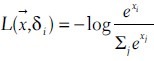
Hence, the outputs of the neural network represent log likelihoods of class membership. The CNN was trained on all positive mitotic figures in the training set, against approximately 1000 randomly chosen negative candidates per ROI. Thus, negatives outnumbered positives by about 16 to 1 in training. To make the CNN classifications more symmetrically invariant, we extended the data set by a factor of eight, by replicating each example flipped or rotated by multiples of 90°. An SVM was trained to classify feature vectors consisting of the features defined above along with the CNN output value. Linear, radial basis function, sigmoid, Laplace, and cubic polynomial models were considered. The model was chosen to maximize F1 score. For both scanners, a Laplace model was most successful.

We now describe our method for extracting mitotic figures using a multispectral microscope affording images from 10 spectral bands and 17 focal planes, each separated by 500 nm. Spectral band 1, which comprises the 410-750 nm range of the spectrum, may be considered as luminance. The other spectral bands are narrower ranges within the visible spectrum. The 10 spectral bands effectively provide a 10-dimensional color space in which PCA may be applied to obtain H and E, color directions, as before. The sequence of eigenvalues is 0.098, 0.016, 0.002,…, supporting the hypothesis that two color channels carry most of the information. Definition of candidate blob sets proceeds as before, using H and E, channels in a favored focal plane (plane 5). Thresholds are tuned for the multispectral scanner. Feature definitions are identical. A CNN is trained to classify 72 × 72 frames centered at the centroid of each candidate blob set. Such a CNN could be trained for any combination of spectral bands and focal planes. Focal planes before 04 and beyond 08 are clearly out of focus and are not considered. In the experiments, we trained CNN using the H and E channels in bands 5-8 (for a total of eight inputs), but observed no difference from training the CNN in band 7 alone. Each CNN resembles the CNN for the other scanners, with the same sequence of layers and kernel sizes. The search for the best number of units for each hidden layer is repeated, and a final SVM is trained on the CNN output and features of the candidate blob set.

RESULTS

The contest provided 35 ROI from 5 slides for use in development, each ROI measuring 512 × 512 microns. A total of 226 ground truth mitotic figures were to be detected in these ROI (224 for the multispectral microscope, due to alignment issues). We used 25 of these ROI for training and held out 10 for validation. In the test set, 100 mitotic figures (98 for multispectral) are hidden across 15 ROI.

Candidate selection produced a set of centers at which to query the CNN and SVM, as marked in blue in Figure 2.

Figure 2.

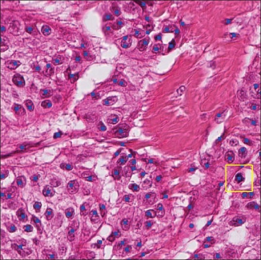
Candidates for classification are marked with square dots. The point classified as mitosis is outlined with a box (Hamamatsu scanner)

The performance of the system on the test set, including the candidate selector, CNN, and SVM, is shown in Table 1. The results include the effect of losing mitotic figures in the candidate selection process (one lost for Aperio; two lost for Hamamatsu; three lost for the multi-spectral scanner).

Table 1.

Performance of system

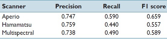
It is remarkable that the multi-spectral results do not greatly surpass those attained on the single spectrum scanners, even if multi-focal or multi-spectral information is utilized. This could reflect the scanner’s image quality.

CONCLUSIONS

We have demonstrated a powerful technique combining segmentation-based features with CNN, identifying the majority of mitotic figures with fair precision.

Through the use of dye color channels and the input flexibility of a CNN, little redefinition was needed to adapt the technique from a single-spectrum, single-focal scanner to a multi-spectral, multi-focal scanner.

CNN afford the possibility of co-training the filters on an auxiliary task, in a supervised[17] or unsupervised fashion.[18] We did not take advantage of these possibilities but limited ourselves to the contest data, particularly to supervised training on the candidates.

The contest data set consists of data from only five distinct slides, with the labels by only one pathologist. We suspect that mitotic figures from the same slide are significantly correlated. Machine learning approaches that generalize well rely on information from identically, independently distributed examples. For a serious application, we recommend that similar techniques be applied to many more slides, with ground truth labels chosen by voting among pathologists, as in Malon et al.[6]

REFERENCES

- 1.Elston CW, Ellis IO. Pathological prognostic factors in breast cancer.I. The value of histological grade in breast cancer: Experience from a large study with long-term follow-up. Histopathology. 1991;19:403–10. doi: 10.1111/j.1365-2559.1991.tb00229.x. [DOI] [PubMed] [Google Scholar]
- 2.Meyer JS, Alvarez C, Milikowski C, Olson N, Russo I, Russo J, et al. Breast carcinoma malignancy grading by Bloom-Richardson system vs proliferation index: Reproducibility of grade and advantages of proliferation index. Mod Pathol. 2005;18:1067–78. doi: 10.1038/modpathol.3800388. [DOI] [PubMed] [Google Scholar]
- 3.Liu A, Li K, Kanade T. IIn Proc IEEE Intl Symp on Biomedical Imaging (ISBI) Netherlands: Rotterdam; 2010. Mitosis sequence detection using hidden conditional random fields; pp. 580–3. [Google Scholar]
- 4.Yang F, Mackey MA, Ianzini F, Gallardo G, Sonka M. Cell segmentation, tracking, and mitosis detection using temporal context. Med Image Comput Comput Assist Interv. 2005;8:302–9. doi: 10.1007/11566465_38. [DOI] [PubMed] [Google Scholar]
- 5.Tao CY, Hoyt J, Feng Y. A support vector machine classifier for recognizing mitotic subphases using high-content screening data. J Biomol Screen. 2007;12:490–6. doi: 10.1177/1087057107300707. [DOI] [PubMed] [Google Scholar]
- 6.Malon C, Brachtel E, Cosatto E, Graf HP, Kurata A, Kuroda M, et al. Mitotic figure recognition: Agreement among pathologists and computerized detector. Anal Cell Pathol (Amst) 2012;35:97–100. doi: 10.3233/ACP-2011-0029. [DOI] [PMC free article] [PubMed] [Google Scholar]
- 7.Elie N, Becette V, Plancoulaine B, Pezeril H, Brecin M, Denoux Y, et al. Automatic analysis of virtual slides to help in the determination of well established prognostic parameters in breast carcinomas (abstract) Anal Cell Pathol. 2011;34:187–8. [Google Scholar]
- 8.Weinstein R, Graham AR, Lian F, Bhattacharyya AK. Z-axis challenges in whole slide imaging (WSI) telepathology (abstract) Anal Cell Pathol. 2011;34:175. [Google Scholar]
- 9.Boucheron LE, Bi Z, Harvey NR, Manjunath B, Rimm DL. Utility of multispectral imaging for nuclear classification of routine clinical histopathology imagery. BMC Cell Biol. 2007;8(Suppl 1):S8. doi: 10.1186/1471-2121-8-S1-S8. [DOI] [PMC free article] [PubMed] [Google Scholar]
- 10.Masood K, Rajpoot NM. Spatial analysis for colon biopsy classification from hyperspectral imagery. Ann Br Mach Vis Assoc. 2008;4:1–16. [Google Scholar]
- 11.Le Cun Y, Bottou L, Bengio Y, Haffner P. Gradient-based learning applied to document recognition. Proc IEEE. 1998;86:2278–324. [Google Scholar]
- 12.Garcia C, Delakis M. Convolutional face finder: A neural architecture for fast and robust face detection. IEEE Trans Pattern Anal Mach Intell. 2004;26:1408–23. doi: 10.1109/tpami.2004.97. [DOI] [PubMed] [Google Scholar]
- 13.Osadchy M, Le Cun Y, Miller ML. Synergistic face detection and pose estimation with energy-based models. J Mach Learn Res. 2007;8:1197–1215. [Google Scholar]
- 14.Lo SB, Lou SA, Lin JS, Freedman MT, Chien MV, Mun SK. Artificial convolution neural network techniques and applications for lung nodule detection. IEEE Trans Med Imaging. 1995;14:711–8. doi: 10.1109/42.476112. [DOI] [PubMed] [Google Scholar]
- 15.Jarrett K, Kavukcuoglu K, Ranzato MA, LeCun Y. What is the best multi-stage architecture for object recognition? In Proc Intl Conf on Comput Vis. 2009:2146–53. [Google Scholar]
- 16.Le Cun Y, Bottou L, Orr GB, Muller KR. Efficient backprop.In neural networks, tricks of the trade. Lect Notes Comput Sci 1524. 1998:9–50. [Google Scholar]
- 17.Ahmed A, Yu K, Xu W, Gong Y, Xing E. Training hierarchical feed-forward visual recognition models using transfer learning from pseudo tasks. In: European Conference on Computer Vision. Part 3. Lect Notes in Comput Sci 5304. 2008:69–82. [Google Scholar]
- 18.Ranzato M, Huang F, Boureau YL, LeCun Y. Unsupervised learning of invariant feature hierarchies with applications to object recognition. IEEE Conference on Computer Vision and Pattern Recognition; 2007. pp. 1–8. [Google Scholar]