Mitosis detection using generic features and an ensemble of cascade adaboosts

Abstract

Context:

Mitosis count is one of the factors that pathologists use to assess the risk of metastasis and survival of the patients, which are affected by the breast cancer.

Aims:

We investigate an application of a set of generic features and an ensemble of cascade adaboosts to the automated mitosis detection. Calculation of the features rely minimally on object-level descriptions and thus require minimal segmentation.

Materials and Methods:

The proposed work was developed and tested on International Conference on Pattern Recognition (ICPR) 2012 mitosis detection contest data.

Statistical Analysis Used:

We plotted receiver operating characteristics curves of true positive versus false positive rates; calculated recall, precision, F-measure, and region overlap ratio measures.

Results:

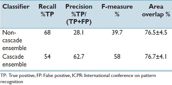
We tested our features with two different classifier configurations: 1) An ensemble of single adaboosts, 2) an ensemble of cascade adaboosts. On the ICPR 2012 mitosis detection contest evaluation, the cascade ensemble scored 54, 62.7, and 58, whereas the non-cascade version scored 68, 28.1, and 39.7 for the recall, precision, and F-measure measures, respectively. Mostly used features in the adaboost classifier rules were a shape-based feature, which counted granularity and a color-based feature, which relied on Red, Green, and Blue channel statistics.

Conclusions:

The features, which express the granular structure and color variations, are found useful for mitosis detection. The ensemble of adaboosts performs better than the individual adaboost classifiers. Moreover, the ensemble of cascaded adaboosts was better than the ensemble of single adaboosts for mitosis detection.

INTRODUCTION

Histopathology became one of those fields, which strongly demand more automated tools to assist the analysis and objective quantification of the images. Mitosis count, which is used to assess the risk of metastasis and survival of the breast cancer patients is one of those problems of histopathology.[1]

To evaluate the risk of metastasis, a mitosis grade of 1-3 is used. The grade is assigned according to the number of mitotic cells, which is counted in a certain number of fields. The mitotic cells are briefly defined as having no nucleus membrane, basophilic cytoplasm, and hairy extensions (Van Diest and Baak criteria).[1] This description can be sufficient for a trained pathology expert; however, it is certainly not well-defined for a computer vision algorithm. First of all, it involves components such as nucleus, cytoplasm of the cells to be segmented. There are some methods in the literature, which work on segmented object-level descriptors.[2] However, segmentation is often a very complicated task and is error prone owing to overlapping cells or open and not clear boundaries of the objects.

The proposed methodology is mainly based on author’s observations on the mitosis dataset, which was made available by the ICPR 2012 Mitosis Detection Contest.[3] There are three different image data sets available in this dataset; however, this work studies only one of the sets (Set A), which had 35 Red, Green, Blue (RGB) images and manually marked ground truth files that show the mitosis sections for each image. After inspecting the images and ground truth data, it was obvious that a cell level segmentation was not feasible, which led to search of some generic features, which can be calculated with minimal segmentation process such as thresholding. These generic features were inspired by similar bio-image analysis works, which aimed at automated microscopy diagnosis.[4,5]

MATERIALS AND METHODS

We study the problem of mitosis detection in a general visual pattern recognition frame-work inspired by modern object detection methodologies like face detectors.[6] A common approach in these works is to train an object detector using the supervised learning methods. This detector can identify whether an object of interest exists in a given image window or not. Then, a sliding window scanner visits each pixel in the image to extract local windows that will be feed to the detector. It is often necessary to scan in different scales to cope with varying sizes of target objects.

Our method follows this approach where we study the dataset first to create a detector. Building of such a detector that is able to identify existence of a mitotic cell in a given image window requires training of a classifier. After the detector is trained, input images are scanned to extract windows for the detector. The detector’s decision is binary and per window or region. This is slightly different than the general sliding window approach where the detector makes a decision for all possible windows of determined sizes around each pixel, which requires a post-process to merge multiple decisions concerning a single object.

Our method can be examined in four different stages: Pre-processing (candidate region detection), feature extraction, classifier construction, and detection.

Pre-Processing (Candidate Region Extraction)

In a typical image, visiting each pixel, to extract its local neighborhood window to be given to the detector is a computationally intensive process. Usually, the number of pixels to visit is around few millions. Visiting each pixel more than one time for different scales will multiply number of windows for the detector to process. To finish the whole analysis of a single image in a reasonable time the window extractor has to be more selective.

Fortunately, an observation of the mitosis regions reveals a simple way to eliminate some of the windows: The mitosis regions in these images are usually darker regions. Figure 1 shows histograms of mitosis sections and non-mitosis random sections extracted from 35 images. Even though, clear boundaries cannot be observed (which may suggest that the detector could be based only on color), it is possible to note that the peaks of green and blue channels of mitotic regions are lower than the peaks of random regions. A morphological double threshold operation is employed here to extract candidate regions. The double threshold operation is the morphological infinite reconstruction (R^δ) of a wider threshold (T_w (I)) from a narrow threshold (T_n (I)) of image I:[7]

Figure 1.

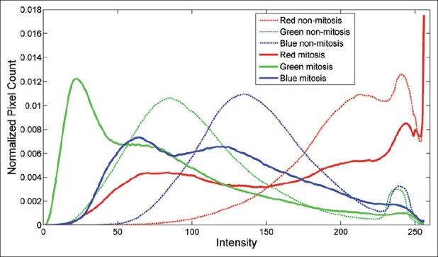
Red, Green, Blue histograms of mitosis versus randomly selected non-mitosis sections

In other words, the double threshold reconstructs any region with at least a single pixel, which satisfies the narrow threshold (T_n (I)), to a connected region comprised of all of its pixels, which satisfy the wide threshold (T_w (I)). Figure 2 shows a 300 × 300 section of one input image with wide and narrow thresholds and corresponding morphological double threshold result. It can be seen that the reconstructed result preserves the regions marked with narrow threshold although removing the rest. This process provides a better way for image thresholding than using a single threshold. Then, a morphological area opening operation removes very small regions. Finally, a hole filling operation fills the regions to complete the pre-process step.[7] The accuracy of this pre-process is discussed in the results section.

Figure 2.

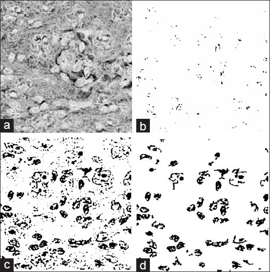
Morphological double threshold operation; (a) original image and the result of; (b) narrow threshold; (c) wide threshold; (d) reconstructed binary image

Feature Extraction

Despite the fact that there are many popular features, which can be used in general object detection tasks (e.g., Haar-like,[6] SIFT[8]), a feature to be used in analysis of microscope images must be strictly a rotation invariant one. After some initial trials we decided to use four different groups of features: Color, binary shape-based, Laplacian, and morphological features. We must note that we avoided using of object level descriptors to avoid the necessity for an object level segmentation process. The color group includes 15 individual simple features such as mean, standard deviation, mode of RGB channels as well as RGB histogram similarities (measured by intersection) to the overall mitosis and non-mitosis section histograms. Here, we use the previously calculated (total) mitosis section histograms as references in the similarity [Figure 1]. The second group of features calculates geometrical features on the candidate region’s binary mask. This set includes 19 individual features such as area, circularity, eccentricity, major-minor axis lengths, and ratio of the area of the largest component to the area of the window. The third group aims to capture textural information by calculating the total intensity reduction between consecutive levels of Laplacian pyramid calculated from the image window. The differences between two consecutive levels are summed over the window to produce the different feature values at different levels.[9]

where DoG stands for difference of Gaussians, * denotes convolution, I shows the input grey level image. The Gaussian kernels have zero mean and variance σ_k. The k^th feature value is simply the sum of the difference image between two consecutive Gaussian convolved images where variance values are shown by σ_k, moreover σ_k /σ_k-1 = 2. The feature calculation is constricted by the local window; however, for efficiency we calculate the Gaussian convolutions once for the entire image, but calculate the sums for the individual windows.

The fourth group aims to capture textural (granular) properties using the area granulometry (or pattern spectra), which was used in similar studies.[4,10] By calculating image’s intensity reduction after a morphological opening operation (the probe), the granulometry calculates the distribution of an image’s similarity to that morphological opening structure of different sizes. Here, we have used the area granulometry with morphological area openings, to extract distribution of different sizes of granular components of the region. The area granulometry (f^ag) of an image can be defined as the total differential mass between consecutive area openings (γ^a) of an increasing area threshold (T (k))[10]

We calculate area granulometry in 20 linearly spaced area thresholds in range (T (k) ∈ [1, WχH]) where W and H are the width and height of the local window respectively (forms a 20 element vector). Finally, the four different groups of features are concatenated to form a vector of 58 values.

Classifier

Extracted features vary largely in their types and produce a 58 dimensional space. Therefore, a strong classifier needs to be constructed. After initial trials, we focused on the adaboost classifier and a cost-sensitive variant.[11,12] Adaboost is a linear combination of selected simple decision stumps. The decision stump is simply an individual feature measurement and a threshold value, which divides that feature space into two separate regions for two classes.

Where α_k is the weight for the decision stump h_k. T denotes decision threshold (default zero) and used to manipulate the decision boundary. Despite its desirable properties (e.g., known as resistant to overfitting) this method suffers from the imbalanced data, which is common to almost every supervised learning system. However, it is possible to search for an appropriate balance of classes by changing the decision threshold T after the training (learning) phase. A variant of adaboost that was developed by Shirazi attacks this problem by modifying the calculation of linear weighting coefficients and the best decision stump with respect to a given cost.[12] Given a cost structure for two target classes [c₁, c₂], Shirazi’s method performs the adaptive boosting of the classifier (and picking the decision stumps) directly with respect to the given costs. However, there is no clear relationship between a desired balanced accuracy (i.e., true positive vs. false positive) and these costs. Therefore, one needs to search for the best cost structure to obtain a desired operating balance.

Nevertheless, Shirazi’s cost sensitive adaboost approach makes it suitable to design cascade classifiers, which are formed of consecutive stages. To reach a given final target true detection and false detection rate, one needs to control the stage classifier’s detection rates. Viola controls the stage classifiers by manipulating their thresholds, whereas Shirazi creates cost aligned optimal adaboosts, which do not need post manipulation.[6,12] In order to create a cascade of adaboost classifiers, we implement a simple approach. We start by using Viola’s method for calculating the necessary stage true positive and false positive rates to reach a goal target true and false positive rate pair (D_T, F_T):

Then, we use Shirazi’s cost sensitive adaboost training to form each stage classifier incrementally, such that in every step a new rule (decision stump) is added to the stage classifier. Then the stage classifier is tested on the training set to note its actual true and false positive rates (d_a, f_a). By assumption the incremental rule addition must stop when the stage targets are achieved (d_a > d_s, f_a < f_s). However, in practice we observed that these constraints are too tight and often not achievable within a reasonable number of rule additions. Hence, we limit the number of rules that can be added to the classifier with a constant value that is gradually increased as the stage level increases. In addition, if maximum number of rules for that level is reached, we accept any rule set that gives the maximum true detection rate d_a among the ones, which satisfy (f_a < f_s).

Another modern technique, we incorporate into our classifier is to create an ensemble of classifiers instead of using a single classifier.[13] In this way, we aim to reduce the false positives. The potential benefit from creating an ensemble is mostly dependent on the variation embedded through the different classifiers forming that ensemble. To practically create an ensemble of classifiers, we divided the training set into 10 folds where the classifiers used 9 random folds to train and remaining other for the validation. The trained individual adaboosts were later merged to have an ensemble decision that is formed by the majority of their votes.

RESULTS

This method was developed and tested on a dataset that is provided by ICPR 2012 Mitosis Detection Contest organization.[3] Despite that there were two other sets made available for the contest, we have only used the image set produced by scanner A which had 35 2048 × 2048 (resolution: 0.2456 μm/pixel) RGB images (hereafter Set-A). The images in Set-A were provided with manually marked ground data, which showed the bounding box for 227 mitosis regions.

Initially, we extracted all the mitosis windows and also some random windows from the images (all 35 images) to calculate RGB histograms. Simple rough observation of the histograms revealed pre-processing thresholds for double threshold operations as (threshold narrow = 80, 50, 80 and threshold wide = 150, 100, 150). Table 1 shows the accuracy of different components of this pre-process. Here, we compare the extracted connected components’ center coordinates with those of ground truth bounding boxes. It can be seen that the application of reconstruction (double threshold) improves both overlap accuracy and precision. Furthermore, we note that the slight variation in the recall values is due to the comparison of the center coordinates rather than the regions (this caused two mitosis regions that are in Telophase state to be incorrectly evaluated as missed). The application of area opening with area threshold of 100 pixels improves the precision further by cleaning some more regions. Owing to the final hole-filling operation the detected region versus bounding box overlap accuracy also increases.

Table 1.

Mean recall and precision for region detection (center coordinates), and region overlap accuracies for pre-processing (candidate extraction)

The pre-process generated 24941 connected component regions (average ~712) from 35 images for further processing (i.e., feature extraction and classification).

In order to provide variations to the learning process to improve the generalization the feature extractor visits every connected component and places a bounding box to define a window. The window size will vary depending on the original region size in addition to a tolerance margin. The margins, which have preset values in the set ({5, 4, 3, 2, 1, 0}) are added to the width and height of the bounding box and the same region is extracted 6 times with bounding boxes of different margins. This process increased the number of total windows to 124,705 (only ~1300 were positive). A feature vector of 58 individual features is calculated for each window.

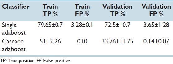
For the classifier construction, we have divided the samples of 35 images into 3 folds of 27-3-5 images, for training, validation, and test respectively. To train the ensembles, each classifier of the ensemble was trained with samples of 27 randomly selected images where samples of remaining 3 images were separated for validation (also to allow more variations). Samples of a randomly selected set of five images were isolated and later used for tests. The settings for individual classifiers were as follows: The non-cascade adaboost classifiers were formed using 200 rules each. On the other hand, the cascade adaboost classifiers were trained for maximum 35 stages unless the false positive rate reached zero in an earlier stage. A decreasing cost structure is used for increasing levels of the cascade: C_mitosis was set 8 for the initial stage and reduced by a factor of 0.95, where C_nonmitosis was set 1 for all stages. Each stage classifier in a cascade could have different number of rules, which was limited by a constant value, which initialized to 4 and reached to 250 (linearly) at the end of 35 stages. Table 2 summarizes the results for the training and validation sets. It can be seen that single adaboost classifier (decision threshold zero) provided more true positives with also more false positives. The cascade adaboosts provided zero false positives on training sets which indicates that the training ended because no more negative samples were left. If we consider the number of visited windows in a typical image a false positive rate more than 0.001 will be very inconvenient. Hence, we favored lower false positives over higher true positives.

Table 2.

Performance for the training and validation sets

We have tested both configurations on the test set of 5 images and calculated receiver operating characteristics (ROC) curves. For the non-cascade version, we have extracted the ROC curve by applying different decision thresholds. For the cascade classifiers we have tested them by allowing the decision stages incrementally. Figure 3 shows the ROC curves plotted from the tests on the set of 5 images. Note that, the set was isolated during training and none of the classifiers had used samples from it. It can be clearly seen that ensemble approach improved both cascade and non-cascade classifiers. It is also clear that cascade ensemble was better than the non-cascade one in both true and false positives. We also observed that before the end stage cascade ensemble could provide better trade-offs for true positive versus false positive rates as final stages seem to cut only on the true positive rate.

Figure 3.

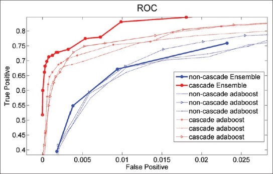
Receiver operating characteristics curves calculated on the test set of five images comparing cascade and non-cascade ensembles formed of nine classifiers each

Finally, we have tested the classifiers on a separate evaluation test set that is provided by ICPR 2012 mitosis detection contest. This set included 15 images including 100 mitosis sections; however, the ground truth file was not shared to contesters and performances were measured by the contest organizers. Table 3 summarizes the results, which evaluate the proposed method from start to end (including the pre-processing) with two different classifiers. In line with our results in the validation set, the recall rate of the non-cascade classifier ensemble is higher although providing almost half of the precision. F-measure is clearly improved with the cascade ensemble. However, our test set ROC promised even better results. This may be due to the final level stages, which reduced true detection without much improvement on the false positive rate. However, we had no chance to extract a ROC for this evaluation set and test this hypothesis before writing of this manuscript.

Table 3.

Performance of the overall method on ICPR 2012 mitosis detection contest evaluation set

Later, we calculated histograms to reveal the utility of different features. We found that the mostly added rule to the adaboosts were based on the binary shape feature “number of connected components in the window, which has less than 10 pixels,” followed by the standard deviation of red and blue channels. Some other popular features were intersection of green channel histogram with the histogram of non-mitosis random section histograms, first level Laplacian feature and the second feature of the area granulometry (this corresponds to area opening with a very small area threshold).

These indicate that a granular structure may be a strong evidence for mitosis appearance: This is mostly expressed with binary features and also the second feature of the granulometry vector. Moreover, color variations are important such that deviations in red channel and blue channel intensity distributions and the histogram comparisons were found useful many times. Area or geometry of large components in the scanned window (obtained by our thresholding) were found not important and were not included in the set of hundreds of rules in the ensembles. However, that can be also related to a possible correlation of that features with some already included ones.

DISCUSSION

The proposed method applied generic features and ensemble of adaboost classifiers to the mitosis detection problem. We believe the generic methodology proposed here is quite successful in the way it introduces new features and tools to the mitosis detection field.

The new features included area granulometry, difference of Gaussians, and histogram intersections with those of mitosis/non-mitosis windows. The study revealed that the features, which expressed the granular structure were most successful compared to the others. It may be possible to include more texture sensitive features in the feature set.[2]

The cascade adaboost ensemble provides an easily controllable true positive/false positive rate by limiting the final effective stage. It is also quite effective since the usual first few stages of the classifiers rely on calculation of few number of features (< 20). In our tests, it provided over 70% recall rate for very low false positives (< 0.1%). In an independent evaluation by contest organizers our non-cascade ensemble classifier version ranked 8^th among 14 other contestants, with an F-measure of 0.39. If the cascade ensemble performance were to be ranked as shown in Table 3 it would take 6^th position.

Despite that our methodology was built, validated, and tested on only the scanner Set-A images, we believe that the same concept can be applied to the other scanners. However, it must be noted that the method presented here is probably vulnerable to illumination color and use of chromatic filters, owing to the color based features which rely on RGB histograms. It may also be affected by significant changes in scale because of some features, which are based on pixel counts. This issues must be addressed by additional phases of pre-processing.[5]

REFERENCES

- 1.Genestie C. Mammary pathology. Tech Report Hospital de la Pitie-Salpetriere. [Last accessed on 2012 Dec 10]. Available from: http://ipal.cnrs.fr/doc/projects/MammaryPathology_CatherineGenestie_2011.pdf .
- 2.Gurcan MN, Boucheron LE, Can A, Madabhushi A, Rajpoot NM, Yener B. Histopathological image analysis: A review. IEEE Rev Biomed Eng. 2009;2:147–71. doi: 10.1109/RBME.2009.2034865. [DOI] [PMC free article] [PubMed] [Google Scholar]
- 3.Roux L, Racoceanu D. Mitosis detection contest. [Last accessed on 2012 Dec 10]. Available from: http://ipal.i2r.a-star.edu.sg/ICPR2012/
- 4.Tek FB, Dempster AG, Kale I. Parasite detection and identification for automated thin blood film malaria diagnosis. Comput Vis Image Underst. 2010;114:21–32. [Google Scholar]
- 5.Tek FB, Dempster AG, Kale I. Computer vision for microscopy diagnosis of malaria. Malar J. 2009;8:153. doi: 10.1186/1475-2875-8-153. [DOI] [PMC free article] [PubMed] [Google Scholar]
- 6.Viola P, Jones MJ. Robust real-time face detection. Int J Comput Vis. 2004;57:137–54. [Google Scholar]
- 7.Soille P. Morphological image analysis: Principles and applications. New York: Springer-Verlag; 1999. [Google Scholar]
- 8.Lowe DG. Distinctive image features from scale-invariant keypoints. Int J Comput Vis. 2004;57:91–110. [Google Scholar]
- 9.Szeliski R. Computer vision: Algorithms and applications. New York: Springer-Verlag; 2011. [Google Scholar]
- 10.Meijster A, Wilkinson MH. Fast computation of morphological area pattern spectra. Proc Int Conf Image Proc. 2001;3:668–71. [Google Scholar]
- 11.Freund Y, Schapire R, Abe N. A short introduction to boosting. J Jpn Soc Artif Intell. 1999;14:1612. [Google Scholar]
- 12.Masnadi-Shirazi H, Vasconcelos N. Cost-sensitive boosting. IEEE Trans Pattern Anal Mach Intell. 2011;33:294–309. doi: 10.1109/TPAMI.2010.71. [DOI] [PubMed] [Google Scholar]
- 13.Duda RO, Hart PE, Stork DG. Pattern classification. New York: Wiley; 2001. [Google Scholar]