

Abstract
This paper investigates the steady hydromagnetic three-dimensional boundary layer flow of Maxwell fluid over a bidirectional stretching surface. Both cases of prescribed surface temperature (PST) and prescribed surface heat flux (PHF) are considered. Computations are made for the velocities and temperatures. Results are plotted and analyzed for PST and PHF cases. Convergence analysis is presented for the velocities and temperatures. Comparison of PST and PHF cases is given and examined.
Introduction
Interest of recent researchers in analysis of boundary layer flows over a continuously moving surface with prescribed surface temperature or heat flux has increased substantially during the last few decades. These flows have abundant applications in many metallurgical and industrial processes. Specific examples of such industrial and technological processes include wire-drawing, glass-fiber and paper production, the extrusion of polymer sheets, the cooling of a metallic plate in a cooling bath, drawing of plastic films etc. Such situations occur in the class of flow problems relevant to the polymer extrusion in which the flow is generated by stretching of plastic surface [1], [2]. In addition, internal heat generation/absorption has key role in the heat transfer from a heated sheet in several practical aspects. The heat generation/absorption effects are also important in the flow problems dealing with the dissociating fluids. Influences of heat generation/absorption may change the temperature distribution which corresponds to the particle deposition rate in electronic chips, nuclear reactors, semiconductor wafers etc. The idea of boundary layer flow over a moving surface was introduced by Sakiadis [3]. He discussed the boundary layer flow of viscous fluid over a solid surface. This analysis was extended by Crane [4] for a linearly stretched surface. He provided the closed form solutions of two-dimensional boundary layer flow of viscous fluid over a surface. Numerous literature now exists on the boundary layer flow with heat transfer and in the presence of heat generation/absorption effects (see [5]–[10] and many refs. therein).
A large number of industrial fluids like polymers, soaps, molten plastics, sugar solutions pulps, apple sauce, drilling muds etc. behave as the non-Newtonian fluids [11]. The Navier-Stokes equations cannot explore the properties of such materials. In the literature, different types of fluids models are developed according to the nature of fluids. The non-Newtonian fluids are mainly divided into three categories which are known as the differential, rate and integral types. The fluid considered here is called the Maxwell fluid. It is subclass of rate type fluids predicting the characteristics of relaxation time. The properties of polymeric fluids can be explored by Maxwell model for small relaxation time. Zierep and Fectecau [12] discussed the energetic balance for the Rayleigh-Stokes problem involving Maxwell fluid. Closed form solutions of unsteady flow of Maxwell fluid due to the sudden movement of the plate was described by Hayat et al. [13]. Fetecau et al. [14] provided the exact solutions for the unsteady flow of Maxwell fluid. Here they considered that the flow is generated due to the constantly accelerating plate. Flow of Maxwell fluid with fractional derivative model between two coaxial cylinders was also addressed by Fetecau et al. [15]. Here the inner cylinder is subjected to the time-dependent longitudinal shear stress generating the fluid motion. Helical unidirectional flows of Maxwell fluid due to shear stresses on the boundary have been studied by Jamil and Fetecau [16]. They provided the exact solution by Hankel transform method. Stability analysis for the flow of Maxwell fluid under soret-driven double-diffusive convection in a porous medium was examined by Wang and Tan [17]. Two-dimensional boundary layer flow of Maxwell fluid over a linearly stretching surface was analyzed by Hayat et al. [18]. Mukhopadhyay [19] presented an analysis for the unsteady flow of Maxwell fluid in a porous medium with suction/injection. Falkner-Skan flow of Maxwell fluid with mixed convection over a surface was analytically discussed by Hayat et al. [20].
The main theme of present analysis is to discuss the steady three-dimensional boundary layer flow of Maxwell fluid over a bidirectional stretching surface subject to prescribed surface temperature and prescribed surface heat flux. The effects of applied magnetic field are also included in this analysis. To our knowledge, not much is known about flows induced by a bidirectional stretching surface. Wang [21] discussed the three-dimensional flow of viscous fluid over a bidirectional stretching surface. Ariel [22] provided the exact and homotopy perturbation solution for ref. [21]. Liu and Andersson [23] discussed the heat transfer analysis over a bidirectional stretching surface with variable thermal conditions. Ahmed et al. [24] extended the analysis of ref. [23] for hydromagnetic flow in a porous medium. They presented the series solutions. Hayat et al. and Shehzad et al. [25], [26] studied the boundary layer flows of Maxwell and Jeffery fluids over a bidirectional stretching surface. The present analysis is arranged as follows. The next section contains the mathematical formulation of the problem. Sections three and four are for the homotopy solutions (HAM) [27]–[34], convergence study and discussion. Both cases of prescribed surface temperature (PST) and prescribed surface heat flux (PHF) are given due attention in the discussion section. The main observations of this research are listed in the last section. Further, the correct modelling for magnetohydrodynamic case of Maxwell fluid is given.
Flow Model
Consider three-dimensional magnetohydrodynamic (MHD) boundary layer flow of an incompressible Maxwell fluid. The flow is induced by bidirectional stretching surface (at  with PST and PHF. Steady flow of an incompressible Maxwell fluid is considered for
  Flow analysis is carried out in the presence of heat generation/absorption parameter. The fluid is electrically conducting in the presence of applied magnetic field with constant strength
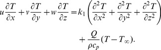
  No electric field contribution is taken into account. Induced magnetic field effects are ignored through large magnetic Reynolds number consideration. The geometry of considered flow is shown in Fig. 1. The conservation of mass, momentum and energy for steady flow in presence of magnetic field and heat source/sink can be expressed as
Figure 1. Physical model.

| (1) |
| (2) |
| (3) |
in which  depicts the density,
  the current density,
  the magnetic field in the
  direction,
  the specific heat,
  the thermal conductivity and
  the heat generation/absorption parameter with
  (heat generation) and
  (heat absorption).
 is a unit vector parallel to the
  axis). The definition of
  for present flow consideration is
| (4) |
where  denotes the fluid velocity and
  the electrical conductivity. The Lorentz force thus reduces to
| (5) |
Expressions of Cauchy  and extra stress
  tensors in Maxwell fluid are [11]:
| (6) |
| (7) |
where  is the Covariant differentiation and
  is the relaxation time. The first Rivilin Ericksen tensor
  is defined as
where * indicates the matrix transpose and the velocity field  here is taken as
| (8) |
The definition of  is [11]
| (9) |
Following the procedure of ref. [11] at pages 221–223 and using above equations, we have the following scalar expressions
| (10) |
 |
(11) |
 |
(12) |
 |
(13) |
 |
(14) |
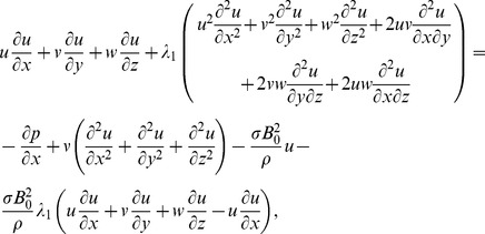
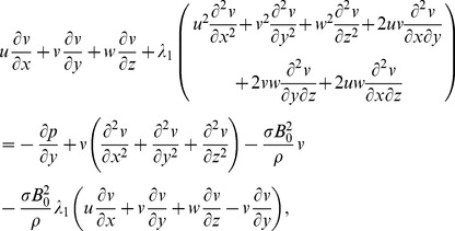
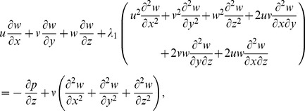
After employing the boundary layer assumptions [35], the above equations in the absence of pressure gradient yield
| (15) |
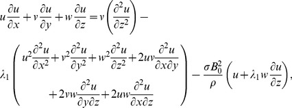 |
(16) |
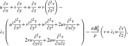 |
(17) |
| (18) |
The associated boundary conditions are defined as follows.
| (19) |
For temperature, the boundary conditions are specified as [23], [24]:
Type i
Prescribed surface temperature (PST)
| (20) |
Type ii
Prescribed surface heat flux (PHF)
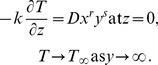 |
(21) |
Here  is the thermal conductivity of the fluid,
  the constant temperature outside the thermal boundary layer,
  and
and  the positive constants. The power indices
  and
and  determine how the temperature or the heat flux varies in the
  plane.
Following [23], [24] similarity variables for the velocity field are introduced as
| (22) |
and the temperature similarity variables take different forms depending on the boundary conditions being considered. These are
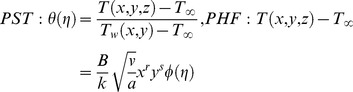 |
(23) |
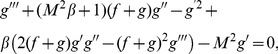
equation (15) is automatically satisfied and Eqs. (16)–(21) take the following forms:
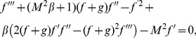 |
(24) |
 |
(25) |
| (26) |
| (27) |
| (28) |
where  is the Deborah number,
  the magnetic parameter,
  the ratio of stretching rates,
  the Prandtl number,
  the thermal diffusivity and
  the internal heat parameter.
Homotopy Analysis Solutions
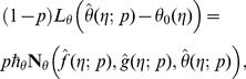
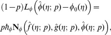
In this section, we solve the problem consisting of Eqs. (24)–(27) with boundary conditions in Eq. (28) by HAM. For that the initial guesses and auxiliary linear operators are taken as follows:
| (29) |
| (30) |
subject to the properties
| (31) |
where 
 are the arbitrary constants.
At zeroth order, the problems satisfy
| (32) |
| (33) |
 |
(34) |
 |
(35) |
 |
(36) |
 |
(37) |
 |
(38) |
 |
(39) |
 |
(40) |
In above expressions,  shows the embedding parameter,

 and
and  the non-zero auxiliary parameters and

 and
and  the nonlinear operators. When
  and
and  then we obtain
 |
(41) |
It should be pointed out that when  increases from
  to
to  then
then 

 and
and  vary from

 to
to 

 and
and  Using Taylors' expansion we write
| (42) |
| (43) |
| (44) |
| (45) |
 |
(46) |
where the parameters 

 and
and  have a key role in the convergence of series solutions. The values of parameters are chosen in such a manner that Eqs.
  converge at
  Hence Eqs.
  give
give
| (47) |
| (48) |
| (49) |
| (50) |
The general solutions are arranged as follows
| (51) |
| (52) |
| (53) |
| (54) |
in which the special solutions are denoted by 

 and
and 
Convergence of Series Solutions and Discussion
It is well known fact that the homotopy analysis method has a great freedom to choose the auxiliary parameters 

 and
and  for adjusting and controlling the convergence of series solutions. To determine the appropriate convergence interval of the constructed series solutions, the
  curves at
  -order of approximations are sketched. Figs. 2 and 3 clearly show that the range of admissible values of

 and
and  are
are 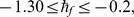
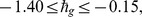
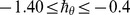 and
and 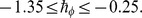
Figure 2.
 curves for the functions
 and
and  when
when 


 and
and  .
.

Figure 3.
 curve for the function
  when
when 


 and
and  .
.

The results are displayed graphically to see the effects of 


 and
and  on the prescribed surface temperature and prescribed surface heat flux. We denote temperature variation for PST case by
  and for PHF situation by
  in the Figs. 4–17. Figs. 4 and 5 illustrate the variations of Deborah number on
  and
and  From these Figs., we have seen that both
  and
and  are increased with an increase in
  Deborah number is based on the relaxation time. When Deborah number increases, the relaxation time increases. This increase in relaxation time causes an increase in
  and
and  Comparison of Figs. 4 and 5 shows that
  has similar effects on
  and
and  Figs. 6 and 7 are plotted to see the effects of magnetic parameter
  on
on  and
and  Clearly the thermal boundary layer thicknesses are increased for larger values of magnetic parameter. In fact the magnetic parameter involves the Lorentz force. Larger values of magnetic parameter correspond to the stronger Lorentz force. This stronger Lorentz force give rise to the thermal boundary layer thicknesses. Figs. 8 and 9 illustrate the variations of
  on
on  and
and  From these Figs. it is noticed that both
  and
and  are reduced when we increased the values of
  Also the thermal boundary layer becomes thinner for higher values of
  This reduction in thermal boundary layer for larger values of
  is due to the entertainment of cooler to ambient fluid. The power indices
  and
and  control the non-uniformity of the surface temperature in the prescribed surface temperature situation. Figs. 10 and 11 depict that
  and
and  are decreasing functions of
  Also we noted that
  reduces rapidly as comparison to
  Effect of
  on
on  and
and  are seen in the Figs. 12 and 13. The values of
  and
and  are reduced when values of
  are increased. It is concluded that the non-uniformity of the sheet temperature has prominent effect on the temperature fields for the reduction in temperature and thinner thermal boundary layer. Comparison of Figs. 12 and 13 illustrates that the variations in
  are more pronounced when compared to the variations in
  Also we examined that
  at the wall reduced rapidly when the values of
  are larger. Figs. 14 and 15 depict the variations of heat generation/absorption parameter
  on
on  and
and  Both
Both  and
and  are increased by increasing values of heat generation/absorption parameter. Physically an increase in heat generation/absorption parameter produced more heat due to which the temperature of fluid increases. This increase in temperature gives rise to
  and
and  The effects of Prandtl number on
  and
and  are analyzed in the Figs. 16 and 17. These Figs. clearly show that
 and their related thermal boundary layer thicknesses are reduced for the larger values of Prandtl number
  Obviously the Prandtl number depends upon the thermal diffusivity. Larger values of Prandtl number give smaller thermal diffusivity and consequently the values of
  and
and  decrease.
Figure 4. Influence of on
on  when
when 


 and
and  .
.

Figure 17. Influence of  on
on  when
when 


 and
and  .
.

Figure 5. Influence of  on
on  when
when 


 and
and  .
.

Figure 6. Influence of  on
on  when
when 


 and
and  .
.

Figure 7. Influence of  on
on  when
when 


 and
and  .
.

Figure 8. Influence of  on
on  when
when 


 and
and  .
.

Figure 9. Influence of  on
on  when
when 


 and
and  .
.

Figure 10. Influence of  on
on  when
when 


 and
and  .
.

Figure 11. Influence of  on
on  when
when 


 and
and  .
.

Figure 12. Influence of  on
on  when
when 


 and
and  .
.

Figure 13. Influence of  on
on  when
when 


 and
and  .
.

Figure 14. Influence of  on
on  when
when 


 and
and  .
.

Figure 15. Influence of  on
on  when
when 


 and
and  .
.

Figure 16. Influence of on
on  when
when 


 and
and  .
.

Table 1 has been prepared to analyze the convergent values of the velocities,  and
and  We have seen that our solutions for velocities converge from 16th order of approximations whereas one needs 25th order of deformations for
  and
and  Hence we need less deformations for the velocities in comparison to temperatures for a convergent solution. Table 2 provides the values of temperature gradient
  for different values of
 and
and  when
when  and
and  One can see that our solutions has an excellent agreement with the previous results in a limiting case [20], [21]. Further, it is observed that the temperature gradient at surface
  becomes positive and reduces for
  and
and  and negative for
  and
and  Table 3 presents the numerical values of
  and
and  for different values of
  and
and  when
when 
 and
and  From this Table we noted that our series solutions have very good agreement with the previous results available in the literature.
Table 1. Convergence analysis of series solutions by numerical data for different order of deformations when 


 and
and  .
.
| Order of deformations | f′′(0) | g′′(0) | θ′(0) | φ′(0) |
| 1 | −1.345900 | −0.592325 | −0.92800 | 0.55000 |
| 10 | −1.341759 | −0.600119 | −0.84012 | 0.50038 |
| 16 | −1.341761 | −0.600122 | −0.83823 | 0.50111 |
| 25 | −1.341761 | −0.600122 | −0.83775 | 0.50128 |
| 30 | −1.341761 | −0.600122 | −0.83775 | 0.50128 |
| 35 | −1.341761 | −0.600122 | −0.83775 | 0.50128 |
| 40 | −1.341761 | −0.600122 | −0.83775 | 0.50128 |
Table 2. Temperature gradient at surface  for different values of
 and
and  with
with  and
and  .
.
| r = s = 0 | r = −2, s = 0 | r = 2, s = 0 | r = 0, s = −2 | r = 0, s = 2 | ||
| [23] | α = 0.25 | −0.665933 | 0.554512 | −1.364890 | −0.413111 | −0.883125 |
| [24] | −0.665927 | 0.554573 | −1.364890 | −0.413101 | −0.883123 | |
| Present | −0.66593 | 0.55457 | −1.36489 | −0.41310 | −0.88312 | |
| [23] | α = 0.50 | −0.735334 | 0.308578 | −1.395356 | −0.263381 | −1.106491 |
| [24] | −0.735333 | 0.308590 | −1.395357 | −0.263376 | −1.106500 | |
| Present | −0.73533 | 0.30858 | −1.39536 | −0.26338 | −1.10649 | |
| [23] | α = 0.75 | −0.796472 | 0.135471 | −1.425038 | −0.126679 | −1.292003 |
| [24] | −0.796470 | 0.135470 | −1.425037 | −0.126679 | −1.292010 | |
| Present | −0.79472 | 0.13547 | −1.42504 | −0.12667 | −1.29200 |
Table 3. Temperature gradient at surface  and
and  for different values of
  and
and  when
when 
 and
and  .
.
| −θ′(0) for PST | φ(0) for PHF | ||||||
| B = −0.2 | B = 0.0 | B = 0.2 | B = −0.2 | B = 0.0 | B = 0.2 | ||
| [23] | Pr = 1.0 | 1.348064 | 1.255781 | 1.148932 | 0.741805 | 0.796317 | 0.870355 |
| [24] | 1.348064 | 1.255780 | 1.148934 | 0.741808 | 0.796318 | 0.870372 | |
| Present | 1.34806 | 1.25578 | 1.14893 | 0.74180 | 0.79632 | 0.87037 | |
| [23] | Pr = 5.0 | 3.330392 | 3.170979 | 3.002380 | 0.300265 | 0.315360 | 0.333069 |
| [24] | 3.330394 | 3.170981 | 3.002384 | 0.300265 | 0.315363 | 0.333071 | |
| Present | 3.33039 | 3.17098 | 3.00238 | 0.30028 | 0.31537 | 0.33308 | |
| [23] | Pr = 10.0 | 4.812149 | 4.597141 | 4.371512 | 0.207807 | 0.217527 | 0.228754 |
| [24] | 4.812151 | 4.597143 | 4.371516 | 0.207809 | 0.217529 | 0.228756 | |
| Present | 4.81215 | 4.59714 | 4.37152 | 0.20781 | 0.21753 | 0.22876 | |
Concluding Remarks
In this study, the three-dimensional MHD flow of Maxwell fluid generated by bidirectional stretching surface is investigated for two cases of prescribed surface temperature (PST) and prescribed surface heat flux (PHF). The effects of applied magnetic field  are also taken into account. Interesting observations of this study can be mentioned below:
Effects of Deborah number
 on
on  and
and  are similar in a qualitative manner.
Both
 and
and  are increasing functions of magnetic parameter
Increase in ratio parameter
 reduces the temperatures and their boundary layer thicknesses.
Temperature for
 case decreases rapidly in comparison to
  case when larger values of
  and
and  are employed.
An increase in heat generation/absorption parameter enhances the temperatures
 and
and 
Our series solutions have an excellent agreement with the previous results in limiting cases.
Funding Statement
This paper was funded by the Deanship of Scientific Research (DSR), King Abdulaziz University, Jeddah under grant no. 10-130/1433HiCi. The authors, therefore, acknowledge with thanks DSR technical and financial support. The funder had no role in the study design, data collection and analysis, decision to publish, or preparation of the manuscript.
References
- 1.Fisher EG (1976) Extrusion of plastics. Wiley, New York.
- 2.Tadmor Z, Klein I (1970) Engineering priciples of plasticating extrusion, in polymer science and engineering series. Van Nastrand Reinhold, New York.
- 3. Sakiadis BC (1961) Boundary layer behavior on continuous solid surfaces: I Boundary layer equations for two dimensional and axisymmetric flow. AIChE J 7: 26–28. [Google Scholar]
- 4. Crane LJ (1970) Flow past a stretching plate, ZAMP. 21: 645–647. [Google Scholar]
- 5. Kazem S, Shaban M, Abbasbandy S (2011) Improved analytical solutions to a stagnation-point flow past a porous stretching sheet with heat generation. J Franklin Institute 348: 2044–2058. [Google Scholar]
- 6. Mukhopadhyay S, Bhattacharyya K, Layek GC (2011) Slip effects on boundary layer stagnation point flow and heat transfer towards a shrinking sheet. Int J Heat Mass Transfer 54: 2751–2757. [Google Scholar]
- 7.Rashidi MM, Pour SAM, Abbasbandy S (2011) Analytic approximate solutions for heat transfer of a micropolar fluid through a porous medium with radiation. Commun Nonlinear Sci Numer Simulat 16 (2011) 1874–1889.
- 8. Hayat T, Shehzad SA, Qasim M, Obaidat S (2012) Radiative flow of a Jeffery fluid in a porous medium with power law heat flux and heat source. Nuclear Eng Design 243: 15–19. [Google Scholar]
- 9. Turkyilmazoglu M (2011) Thermal radiation effects on the time-dependent MHD permeable flow having variable viscosity. Int J Thermal Sci 50: 88–96. [Google Scholar]
- 10. Makinde OD, Aziz A (2011) Boundary layer flow of a nonofluid past a stretching sheet with a convective boundary condition. Int J Thermal Sci 50: 1326–1332. [Google Scholar]
- 11.Harris J (1977) Rheology and non-Newtonian flow. Longman, London.
- 12. Zierep J, Fetecau C (2007) Energetic balance for the Rayleigh – Stokes problem of a Maxwell fluid. Int J Eng Sci 45: 617–627. [Google Scholar]
- 13. Hayat T, Fetecau C, Abbas Z, Ali N (2008) Flow of a Maxwell fluid between two side walls due to a suddenly moved plate. Nonlinear Analysis: Real World Applications 9: 2288–2295. [Google Scholar]
- 14. Fetecau C, Athar M, Fetecau C (2009) Unsteady flow of a generalized Maxwell fluid with fractional derivative due to a constantly accelerating plate. Comput Math Appl 57: 596–603. [Google Scholar]
- 15. Fetecau C, Fetecau C, Jamil M, Mahmood A (2011) Flow of fractional Maxwell fluid between coaxial cylinders. Arch Appl Mech 81: 1153–1163. [Google Scholar]
- 16. Jamil M, Fetecau C (2010) Helical flows of Maxwell fluid between coaxial cylinders with given shear stresses on the boundary. Nonlinear Analysis: Real World Applications 11: 4302–4311. [Google Scholar]
- 17. Wang S, Tan WC (2011) Stability analysis of Soret-driven double-diffusive convection of Maxwell fluid in a porous medium. Int J Heat Fluid Flow 32: 88–94. [Google Scholar]
- 18. Hayat T, Shehzad SA, Qasim M, Obaidat S (2011) Steady flow of Maxwell fluid with convective boundary conditions. Z Naturforsch A 66a: 417–422. [Google Scholar]
- 19. Mukhopadhyay S (2012) Upper-convected Maxwell fluid flow over an unsteady stretching surface embedded in porous medium subjected to suction/blowing. Z Naturforsch A 67a: 641–646. [Google Scholar]
- 20. Hayat T, Farooq M, Iqbal Z, Alsaedi A (2012) Mixed convection Falkner-Skan flow of a Maxwell fluid. J Heat Transfer-Trans ASME 134: 114504. [Google Scholar]
- 21. Wang CY (1984) The three-dimensional flow due to a stretching sheet. Phys Fluids 27: 1915–1917. [Google Scholar]
- 22. Ariel PD (2007) The three-dimensional flow past a stretching sheet and the homotopy perturbation method. Comput Math Appl 54: 920–925. [Google Scholar]
- 23. Liu IC, Andersson HI (2008) Heat transfer over a bidirectional stretching sheet with variable thermal conditions. Int J Heat Mass Transfer 51: 4018–4024. [Google Scholar]
- 24. Ahmad I, Ahmed M, Abbas Z, Sajid M (2011) Hydromagnetic flow and heat transfer over a bidirectional stretching surface in a porous medium. Thermal Sci 15: S205–S220. [Google Scholar]
- 25. Hayat T, Shehzad SA, Alsaedi A (2012) Study on three dimensional flow of Maxwell fluid over a stretching sheet with convective boundary conditions. Int J Physical Sci 7: 761–768. [Google Scholar]
- 26. Shehzad SA, Alsaedi A, Hayat T (2012) Three-dimensional flow of Jeffery fluid with convective surface boundary conditions. Int J Heat Mass Transfer 55: 3971–3976. [Google Scholar]
- 27. Liao SJ (2009) Notes on the homotopy analysis method: Some definitions and theorems. Commun Nonlinear Sci Numer Simulat 14: 983–997. [Google Scholar]
- 28. Turkyilmazoglu M (2012) Solution of the Thomas-Fermi equation with a convergent approach. Commun Nonlinear Sci Numer Simulat 17: 4097–4103. [Google Scholar]
- 29. Turkyilmazoglu M (2012) The Airy equation and its alternative analytic solution. Phys Scr 86: 055004. [Google Scholar]
- 30. Turkyilmazoglu M (2011) Convergence of the homotopy perturbation method. Int J Nonlinear Sci Numer Simulat 12: 9–14. [Google Scholar]
- 31. Turkyilmazoglu M (2011) Numerical and analytical solutions for the flow and heat transfer near the equator of an MHD boundary layer over a porous rotating sphere. Int J Thermal Sci 50: 831–842. [Google Scholar]
- 32. Rashidi MM, Keimanesh M, Rajvanshi SC (2012) Study of pulsatile flow in a porous annulus with the homotopy analysis method. Int J Numer Methods Heat Fluid Flow 22: 971–989. [Google Scholar]
- 33. Hayat T, Shehzad SA, Alsaedi A, Alhothuali MS (2012) Mixed convection stagnation point flow of Casson fluid with convective boundary conditions. Chin Phys Lett 29: 114704. [Google Scholar]
- 34. Hayat T, Shehzad SA, Alsaedi A (2012) Soret and Dufour effects on magnetohydrodynamic (MHD) flow of Casson fluid. Appl Math Mech-Engl Edit 33: 1301–1312. [Google Scholar]
- 35.Schichting H (1964) Boundary layer theory. 6th edition, McGraw-Hill, New York.