Trade-off between curvature tuning and position invariance in visual area V4

Abstract

Humans can rapidly recognize a multitude of objects despite differences in their appearance. The neural mechanisms that endow high-level sensory neurons with both selectivity to complex stimulus features and “tolerance” or invariance to identity-preserving transformations, such as spatial translation, remain poorly understood. Previous studies have demonstrated that both tolerance and selectivity to conjunctions of features are increased at successive stages of the ventral visual stream that mediates visual recognition. Within a given area, such as visual area V4 or the inferotemporal cortex, tolerance has been found to be inversely related to the sparseness of neural responses, which in turn was positively correlated with conjunction selectivity. However, the direct relationship between tolerance and conjunction selectivity has been difficult to establish, with different studies reporting either an inverse or no significant relationship. To resolve this, we measured V4 responses to natural scenes, and using recently developed statistical techniques, we estimated both the relevant stimulus features and the range of translation invariance for each neuron. Focusing the analysis on tuning to curvature, a tractable example of conjunction selectivity, we found that neurons that were tuned to more curved contours had smaller ranges of position invariance and produced sparser responses to natural stimuli. These trade-offs provide empirical support for recent theories of how the visual system estimates 3D shapes from shading and texture flows, as well as the tiling hypothesis of the visual space for different curvature values.

Although object recognition feels effortless, it is in fact a challenging computational problem (1). There are two important properties that any system that mediates robust object recognition must have. The first property is known as “invariance”: the ability of the system to respond similarly to different views of the same object. The second property is known as “selectivity.” Selectivity requires that systems' components, such as neurons within the ventral visual stream, produce different responses to potentially quite similar objects (such as different faces) even when presented from similar viewpoints. It is straightforward to make detectors that are invariant but not selective or selective but not invariant. The difficulty lies in how to make detectors that are both selective and invariant.

To address this problem, both computer object recognition algorithms (2) and neural systems use a series of hierarchical stimulus representations, increasing both in complexity and the range of invariance (1, 3). For example, in each successive area of visual processing, neurons become selective for increasingly complex stimulus features (4–9) and grow more tolerant to identity-preserving transformations, such as image translation, scaling, and, to some degree, rotation and the presence of “clutter” from other objects in the scene (3, 10–12). This has led to the idea that high-level sensory neurons are simultaneously selective for complex stimulus features, such as the features of a face (13), and are invariant in that they maintain their responses regardless of where within the visual field the face might appear. However, a study of neural responses in the ventral visual stream found that a high degree of selectivity is inversely related to the degree of tolerance (1, 3, 10), although other studies have found neurons that exhibit high tolerance and high selectivity (see, e.g., ref. 14). Complicating matters, the relationship between invariance and conjunction selectivity can depend on a particular measure of activity that is used as proxy to quantify the complexity of features that drive each neuron (1, 3, 10). This raises the question as to what neural architectures can ultimately sustain reliable object recognition, a question that is also currently at the forefront of computer vision (15, 16).

To provide constraints helpful in addressing this question we focused on the area V4, an intermediate area within the visual object recognition pathway that collects signals from areas V1 and V2 and provides input to the inferotemporal cortex. V4 neurons have previously been shown to be selective to curvature (17–20). This type of feature selectivity provides a simple and quantitatively tractable framework to study conjunction selectivity. Recent statistical techniques make it possible to simultaneously estimate both the types of features that drive each neuron and the range of translation invariance from the neural responses to natural stimuli (21). Here, we applied these techniques to V4 neuronal responses to natural stimuli. The results revealed a number of trade-offs: We find many neurons with limited invariance and relatively few highly invariant neurons in V4. Second, neurons selective for tighter curvatures had smaller ranges of position invariance. These trade-offs can help explain the wide range of sparseness values that have been observed in V4 (1) and help resolve disagreements about the existence of a relationship between invariance and conjunction selectivity. Furthermore, these results support the processing of visual shapes in terms of shading and texture flows.

Results

Our goal was to determine the stimulus features that drove responses of each neuron and the degree of tolerance to changes in the position of each neuron’s preferred features. We probed each V4 neuron with a large number of frames from natural movies (∼30,000 on average, a minimum of 6,000 and a maximum 85,000). Frames were presented in groups of ∼100 as part of ∼3.7-s-long movies. From these responses to natural stimuli, we estimated which of the stimulus features modulated the probability of spiking (either positively or negatively) of a given neuron. We will refer to these features as “relevant stimulus features.” We also estimated each neuron’s invariance to translation from its responses to natural scenes. Both invariance and relevant stimulus features were determined using an extension of the traditional linear–nonlinear (LN) model framework (22, 23). In its simplest form, an LN model accounts for the neural response through a nonlinear function of the similarity between the stimulus and the neuron’s relevant stimulus feature, which also corresponds to the receptive field of the neuron. Generalizations of this approach allow for sensitivity in the neural response to multiple stimulus features (24–28). Here, we have further generalized the approach to take into account the observation that V4 neurons exhibit some degree of position invariance. We incorporated model parameters to allow a variable degree of translation invariance. By allowing these parameters to vary, we estimated the degree to which each neuron exhibited these two forms of invariance. We refer to this as a translation-invariant LN model, and to the corresponding relevant stimulus features as the maximally informative invariant dimensions (MIIDs) because these dimensions were those that, when allowed to vary in position, capture the maximal amount of information about the neural response. Fig. 1A illustrates schematically one way translation-invariant conjunction selectivity could be implemented (29–32). Most of the analyses presented here will be focused on models with partial translation invariance taking into account interactions between two MIIDs. We also compared these models to those with an unlimited range of translation invariance (20) and find that models with unlimited translation invariance (schematized in Fig. S1) yielded the best description of the neural responses of a subset of V4 neurons (see Fig. 4).

Fig. 1.

Estimating feature selectivity of V4 neurons with natural stimuli. (A) Schematic representation of LN models used to characterize feature selectivity and invariance of V4 neurons. Shown here is an LN model with two relevant stimulus features that, in conjunction, can trigger the neural response when positioned at a number of different locations within the visual field. (B and C) Feature selectivity of example V4 neurons with smaller (B, 6%) and larger (C, 12%) ranges of position invariance, respectively. The range of position is measured relative to the spatial field that is shown in B and C encompassing the relevant stimulus features. Color maps indicate the first (Upper) and second (Lower) most relevant stimulus features. The color scale indicates values (either positive or negative) relative to the mean luminance, divided by the average SD across different pixels obtained from different jackknife estimates. The red scale bar is 1°. The overlaid contour plots were obtained by fitting curved 2D Gabor functions to the relevant stimulus features. Neurons m17b_1 (B) and j46a_1 (C). (D) Trade-off between curvature and invariance in V4. The curvature index 1 here is the curvature parameter from the fitted curved Gabor models normalized such that the stimulus frame size has a unit length of 1. We find that this curvature index decreases with the range of position invariance for both the first MIID (gray triangles) and the second MIID (open circles). The solid line shows the least-square fit for all points (P = 0.005 linear correlation); the dashed line is the fit just through points for the first MIID (P = 0.042, linear correlation).

Fig. 4.

Predictive power of LN models with position invariance. (A) The distribution of the percent of mutual information explained by LN models with a variable range of position invariance. (B) A comparison of information explained by the best model to the overall (model-free) information contained in the firing rate. The solid line at 45° corresponds to the case in which all of the information is explained. (C) The distribution of optimal translation ranges across the population of V4 neurons suggests that fewer neurons are needed to represent the visual space when they have wider range of translation invariance.

The relevant stimulus features are determined based on an analysis of the number of spikes that was elicited by each movie frame. The starting point for the analysis is the computation of the spike-triggered average (33), followed by optimization to remove correlations present in the natural stimuli (34). The size of the considered visual area over which signals are pooled determines the range of the position invariance and is an adjustable parameter of the model. Fig. 1 B and C shows the pair of MIIDs for two example neurons obtained using this approach. Here, the color of each pixel indicates the light intensity (darker or lighter, relative to mean background luminance) that maximally modulated the probability of spiking. The spatial profile of each MIID thus corresponds to the pattern of light that, when allowed to translate, maximally modulated the probability of spiking.

We find that many neurons, such as the example neuron in Fig. 1B, were selective for curved contours. This is consistent with previous reports of bimodal orientation tuning in the Fourier domain observed in experiments with natural stimuli (20) and with previous studies using synthetic stimuli (17). The use of natural stimuli here allowed us to use the same stimulus sequence to determine both the feature selectivity and invariance properties of many different neurons.

Trade-Off Between Curvature Tuning and Position Invariance.

Comparing neurons with different ranges of position invariance (measured relative to the spatial extent of MIIDs profiles), we found that neurons with smaller ranges of position invariance were selective for contour elements with tighter curvature. Examples shown in Fig. 1 illustrate this trend. The neuron in Fig. 1B had a smaller range of position invariance. The MIIDs indicate that this neuron was selective for a curved contour. The neuron in Fig. 1C had a larger range of position invariance and its two MIIDs indicated selectivity for an almost straight contour. To characterize curvature selectivity quantitatively and across the population, we fitted the MIIDs for each neuron with a curved Gabor model, as indicated by the overlaid contours plots. Fifty-seven neurons in our population were successfully fit by a model with partial translation invariance. Among these, the MIIDs of 38 neurons (67%) could be well described by the curved Gabor model that we used to estimate curvature tuning (Materials and Methods). Across this subset of 38 neurons, preferred curvature and position invariance were significantly anticorrelated (Fig. 1D). Here, curvature values and the range of position invariance were measured relative to the size of the receptive field. In these relative units, there was no dependence of invariance on eccentricity or clustering of curvature values in retinotopic coordinates (Fig. S2). Thus, the finding of smaller preferred curvature observed in neurons with larger range of position invariance does not necessarily imply that only neurons with small receptive field sizes are selective for large curvature values.

We undertook several control analyses to rule out the possibility that the observed decrease in preferred curvature with position invariance was due either to the particular the way receptive fields were estimated from neural responses to natural stimuli or how they were fitted with the curved Gabor model. First, we created model neurons in which we could independently control the model neuron’s curvature turning and invariance properties. When identical analyses were applied to a set of model cells whose curvature was independent of the range of translation invariance (and should therefore exhibit no correlation between these properties), our analysis found no correlation (Fig. S3). Finally, there was no significant difference in the mean firing rates between neurons with different ranges of position invariance (Fig. S4A) and the corresponding models accounted for a similar fraction of variance/information in the neural responses regardless of the optimal range of position invariance (Fig. S4 B and C). These control analyses show that the observed trade-off between curvature tuning and position invariance in V4 is not due to the estimation procedure.

In thinking about possible mechanisms that might endow V4 neurons with different relative ranges of position invariance, one can envision two scenarios. The first is that different V4 neurons pool signals in a spatially similar way but have different thresholds for spiking (Fig. 2A). For example, a V4 neuron that is selective for a vertical orientation can pool signals originating in V1 simple cells selective for that same vertical orientation but centered at different positions in the visual space. Then, having a higher threshold for spiking would make the V4 neuron respond to the presence of the vertical edge in an image over a smaller range of spatial positions than a V4 neuron with a lower threshold. This possibility predicts that there should be (i) a negative correlation between the threshold value and invariance and (ii) a positive correlation between threshold value and sparseness in the neural responses. To test for these relationships, we computed for each neuron its threshold value (Materials and Methods). The data showed that whereas the negative correlation between thresholds and the range invariance was present (Fig. 2C) there was no relationship between threshold value and sparseness in the neural responses (Fig. 2D). [Note that we observed the same lack of correlation with threshold values when sparseness in the neural responses was quantified using the mutual information contained in the firing rate (Fig. S5A).] These findings therefore point to an alternative mechanism for generating position invariance in V4, where neurons with a smaller range of position invariance receive a set of stronger signals from a more narrow range of spatial location compared with the more distributed pooling in neurons with broader ranges of position invariance (Fig. 2B). If the value of threshold were proportionately scaled with the maximum strength of the inputs, then one would still expect a negative relationship between the threshold and invariance yet no correlation between threshold and sparseness. Thus, it is the second scenario illustrated in Fig. 2B that is consistent with all of the observations.

Fig. 2.

The effect of threshold for spiking on position invariance and sparseness. Two competing models are schematically represented. (A) The range of position invariance is determined by threshold. (B) Position invariance is determined by the range of inputs in space; threshold is scaled proportionately to the strongest input. (C) Negative correlation between threshold and invariance range (P = 0.004, linear correlation) is consistent with both models. Each point is a V4 neuron. (D) Threshold and sparseness are uncorrelated (P = 0.37), which is consistent with model B and not A. (E) Sparseness is larger for neurons that were best described by models with zero position invariance than for neurons best described by models with limited (from 5% to 15%) position invariance (P = 0.0027, Mann–Whitney test). The decrease of sparseness with invariance range x was better described by an inverse quadratic function (solid line shows the best fit) rather than a linear function; P = 0.03, correlation between invariance range and

The sparseness in the neural response can be affected not only by the value of threshold to spike but also by how often the relevant stimulus feature appears in natural scenes. Previous studies found a trade-off between sparseness and invariance in both inferotemporal cortex (IT) (10) and V4 (1). We have also observed similar phenomena in our dataset using two different measures of sparseness (Fig. 2E and Fig. S5). The fact that tighter curvatures are observed less frequently in the natural environment (Fig. S6) together with the inverse relationship between curvature and invariance (Fig. 1D) can help explain how sparseness can be inversely related to invariance, even though it is not affected by changes in threshold (Fig. 2D).

To gain further insights into curvature processing carried out by V4 neurons, one can compare other parameters, such as orientation, spatial frequency, and phase of the curved Gabor model for the two MIIDs of each neuron. For example, V1 complex cells have subunits that have similar orientation and spatial frequency but different spatial phases. This property suggested that V1 complex cells pool signals from simple cells tuned to the same orientation and spatial frequency but different spatial phases (35). Random variation in spatial phase, when pooled, could also contribute to spatial invariance of complex cells. At the same time, end-stopped cells in V1 could encode curvature by combining inputs from simple cells with different preferred spatial frequencies (36). We found a reminiscent pattern in V4. Although across our population of V4 neurons there was a wide range of preferred spatial frequencies and orientations, most commonly the values were similar for the two MIIDs for each (Fig. 3 A and B). At the same time, the relative spatial phase between MIID1 and MIID2 was large, which spanned the range from 0° to 90°, with the median on 53° (Fig. 3A, Inset). Thus, we find in V4 the types of pair selectivity with respect to curved contours that generalized the conjunction selectivity typical of V1 complex cells. At the same time, there were some V4 neurons for which the two MIIDs had similar spatial phase but significantly different preferred orientations. The selectivity to conjunctions of curved features with different preferred orientation could be a signature of selectivity for a type of texture flow (37) where curvature and orientation vary in a coordinated way with spatial position.

Fig. 3.

The two relevant features often form “quadrature” pairs. Across the population, the two relevant stimulus features have on average the same preferred orientation (A) and spatial frequency values (B). The corresponding P values are 0.44 and 0.59 for linear correlation. Points represent different neurons and are colored by the difference between MIID1 and MIID2 of the same neuron in terms of spatial phase (A) and preferred orientation (B). (Inset) Histogram of phase differences between MIID1 and MIID2 shows a peak at ∼50°, reminiscent of selectivity to a quadrature pair of relevant stimulus features typical of V1 complex cells.

Predictive Power.

We find that the derived LN models accounted for a large percentage of the mutual information carried by independent spikes, ranging from 25% to 99.8% (Fig. 4A). Mutual information is a measure that is proportional to the log likelihood of the LN model (38). It should be noted that these percentages relate to the amount of “explainable variance.” This is because variation in the response that does not vary with the stimulus (“noise”) carries zero information about the stimulus. Another important point is that these values were computed using parts of the dataset that were not used to either fit parameters of LN models or find the optimal range of position invariance. Thus, the information values are not affected by overfitting. Similar results were obtained in terms of the percentage of explained variance (P = 0.74, t test for comparison between information and variance explained values). On average, 59% of the information could be explained, which is equal to or greater than that of the state-of-the-art LN models built to describe the V1 neural responses (8, 20). We emphasize that models of V4 neurons were obtained with the same stimulus set as was used in an earlier V1 study (39) and were evaluated in both cases with the same measure of mutual information, allowing for direct comparison between areas. We believe that the improved predictive power of the V4 model is due, in part, to the incorporation of translation invariance. On average, this improved predictive power by 42% (P = 0.0004, t test; comparison was made across 38 neurons whose responses could be predicted above chance by models with or without translation invariance).

We also examined the predictive power of models that incorporated perfect translation invariance and found that they did not typically perform as well as models whose invariance was allowed to vary. Models incorporating limited translation invariance (<15% of the stimulus frame size) proved to be superior to those with perfect translation invariance (those where the MIID was held constant across visual field). The mean gain in predictive power was 38% between models of variable range of translation invariance vs. models with unlimited range of translation (P = 0.0017, t test; comparison was made across 38 cells whose responses could be predicted above chance by at least one of the models). Thus, incorporation of variable-range translation invariance led to substantial improvements in predictive power of models of V4 responses, relative to perfectly translation-invariant models.

How was the range of position invariance distributed across the population of V4 neurons? The majority of V4 neurons were best described by models with nonzero but limited translation invariance (57 out of 109 neurons; Fig. 4C). The next-largest group was neurons that were best described by models with no translation invariance (36 out of 109 neurons). Finally, models with unlimited position invariance were best for 16 out 109 neurons. Neurons with smaller degrees of translation invariance were more numerous than those with greater translation invariance (Fig. 4C). This could potentially reflect the need to tile visual space: Fewer neurons may be needed if they respond to their preferred feature across a wider range of positions. Note that this would predict that cells tuned to shallower curvatures would be less numerous than cells tuned to tighter curvatures (relative to the receptive field size). A direct verification of this prediction was not possible because the fitting procedure for estimating curvature becomes less reliable with increasing curvature value relative to the receptive field size. Therefore, although the distribution of preferred curvature values across the population of V4 neurons shows the preponderance of tuning to shallow curvatures (Fig. S7), one should keep in mind that cells tuned to tighter curvatures are disproportionately eliminated from this histogram and not take its properties as an argument against the tiling hypothesis.

Discussion

The primary goal of this work was to study the relationship between the complexity of neural feature selectivity and its tolerance to translation in the context of natural vision. After deriving relevant stimulus features from the responses of neurons in area V4 to natural stimuli, we focused on the relationship between curvature tuning and position invariance, properties that are amenable to quantification and have been previously shown to be important for image representation in V4 (8, 17, 18, 40). We found that incorporation of a degree of translation invariance into models of V4 neurons substantially improved their ability to account for the neuronal response. We found that most neurons exhibited at least some degree of position invariance, but that only a small fraction of V4 neurons were best described by models with unlimited invariance. Quantifying curvature selectivity, we found that MIIDs could be well fit by curved contours in approximately two-thirds of the neurons. Among neurons with some degree of translation invariance that could be assigned a curvature preference value, neurons with larger position tolerance were tuned to contours of smaller curvature (Fig. 1D).

This study was carried out using natural stimuli. The demonstration provided here that curved contours were the preferred stimulus feature for many neurons thus extends previous reports on the importance of curvature representation in V4 (17, 19, 41) to the natural context. Our results also follow up on the pioneering studies (20) that demonstrated bimodal orientation tuning consistent with the selectivity to curvature. At the same time, the receptive fields that were observed in the present study often were too complex to be described well by a (curved) Gabor model. Future studies will have to examine how such receptive fields relate to other image characteristics that go beyond curvature (8). An encouraging point is that, altogether, position-invariant models described here provided a match to V4 responses similar to that provided by position-specific models for V1 responses (39). These findings suggest that the exploration of high-level sensory areas using diverse natural stimuli and invariant models may be simpler than previously thought (8).

The relationship between conjunction selectivity, invariance, and sparseness has been the focus of several recent studies (1, 3, 10). In both V4 and IT, sparseness is inversely related to tolerance and positively correlated with conjunction selectivity. However, the direct relationship between conjunction selectivity and tolerance has been harder to establish: It was observed in some studies (10), but not others (1). The differences were likely due to different measures used to characterize conjunction selectivity. For example, when conjunction selectivity was measured according to how fast the neural responses deteriorated with the degree of perturbation of the preferred shape for a given neuron (a quantity termed “morph tuning”), an inverse relationship was observed between shape tuning and invariance (10). However, when conjunction selectivity was assessed by comparing the range of the neural responses elicited by natural or scrambled stimuli, no relationship was observed between conjunction selectivity and invariance (1). The present results are consistent with the conclusion that invariance is inversely related to conjunction tuning, in the following sense. We characterized curvature tuning of V4 neurons. Curvature tuning requires the conjunction of orientation-selective responses, presumably originating from orientation-selective V1 neurons. Curvature tuning is, in this sense, analogous to selectivity for conjunctions of the preferred curve’s constituent orientations. Our finding of an inverse relationship between curvature tuning and invariance is therefore consistent with the earlier studies, which showed an inverse relationship between conjunction selectivity and position invariance.

The finding of an inverse relationship between curvature preference and translation invariance is consistent with a recent theory for the computation of 3D shapes from shading flows (42). One of the aspects of that theory is that the shape perception may arise as a result of integration of neural signals corresponding to different elementary shading flows, each of which corresponds to a different orientation and curvature of a possible patch of the 3D surface (43). To avoid error accumulation in simulations, shading flows with larger curvature have to be more limited in spatial extent compared with shading flows with smaller curvature values. Because curved surfaces give rise, in their 2D projection, to curved contours, this theoretical feature of the estimation of 3D shape from shading is thus consistent with the observed trade-off between curvature tuning and position invariance.

The observation of a trade-off between curvature and invariance has another important implication for image representations within the visual stream. Specifically, it refines a hypothesis for how shape tuning in V4 may be formed based on signals from earlier visual areas. Recent physiological studies show that V4 receptive fields are obtained by pooling from a constant area of V1 surface (44). Our results further suggest that the degree to which a given V4 neuron pools signals representing the same orientations centered at different positions or from different orientations within the same visual area will determine its level of selectivity and invariance within a continuous spectrum of shape representations. However, it is unlikely that the differences in V4 selectivity and invariance can be simply explained by differences in the homogeneity of preferred orientation values within the part of V1 that sends signals to a given V4 neuron, for the following reasons. First, selectivity for curvature requires a coordinated change in the preferred orientation and spatial position; such a change would not arise simply by pooling from an area of V1 that contains a pinwheel in its orientation map. Second, each V4 neuron was previously shown to pool signals from a large area of V1 surface, where as much as one-sixth of V1 surface can contribute inputs to a single V4 neuron (44). Indiscriminate sampling from such a large area of V1 surface, containing many pinwheels, is sure to destroy any complex feature selectivity without yielding invariance. Finally, we found no evidence for clustering in curvature preferences or a change with eccentricity for the preferred values of curvature and invariance range, when both quantities were measured in units of the receptive field size. Thus, although V4 neurons pool from vast regions of V1 surface, this pooling has to be highly coordinated to yield the trade-off between curvature tuning and position invariance.

Materials and Methods

Experimental data were collected using procedures approved by the Institutional Animal Care and Use Committee of Salk Institute for Biological Studies and in accordance with National Institutes of Health guidelines. Experimental and surgical procedures have been described previously (45).

Data Collection.

Neural responses to segments of natural movies were recorded in area V4 in two monkeys as they maintained fixation, for a juice reward. Receptive fields were mainly in the right visual field near the fovea. The neural responses were collected extracellularly with tungsten microelectrodes (45). The natural stimulus had a fixed size (14° × 14°) and was placed at the center of the estimated receptive field for each neuron.

Stimuli and Experimental Design.

Natural stimuli consisted of movie segments with approximate duration of 3.7 s. These stimuli were presented at 120 Hz with a frame update rate of 30 Hz within a receptive field of a neuron. Neurons were probed with several hundred such movie segments (range from 52 to 765 movie segments, average 300, median 271). Three movie segments were chosen to be repeated multiple times (“repeated data,” 30 times on average for each of the chosen movie segments, up to 266 times across the three repeated segments). These repeated movie segments were interleaved with those that were presented once (“unrepeated data”). Stimuli and the neural responses were binned at 66-ms resolution. The relevant stimulus features were analyzed at the latency of one time bin before a spike, which corresponds to the latency of visual signals to arrive in the area V4. In this work, we focus on spatial representation of visual signals. Additional time lags were not considered to allow for adequate sampling of receptive field profiles. Typically, the number of recorded spikes should be greater than the number of points in the grid over which receptive fields are estimated. Including additional time lags would have reduced the number of neurons in which receptive fields could be reliably estimated.

The unrepeated dataset was used to fit the LN models of neural responses. The repeated data were split in two halves across the number of presentations, the first of which was used to select the best LN model (according to the type and range of invariance) for each neuron based on the amount of information explained, and the second of which was used to evaluate performance of this optimal model. In this way, the measurements of predictive power are not influenced in any way by either the model selection or its fitting. For analyses that did not involve predictive power, such as comparison between curvature tuning and translation invariance, all of the repeated data were used to determine the range of position invariance.

Structure of Invariant Models for Characterizing V4 Responses.

Each neuron’s responses were fit to maximize the mutual information accounted for by LN models that varied in the range of position invariance (21) and were thus extensions (Fig. 1 and Fig. S1) of the classic LN model (22, 23) to the neural responses. The standard LN model accounts for the neural response through an arbitrary nonlinear function of stimulus projections on a set of a few relevant features. We assume that translation invariance is achieved by pooling across input neuron populations. To model this, we combined multiple LN models, such that the final spiking output of the neuron under study represents a MAX operation on the output of intermediate position-specific LN models that represent input neurons (similar procedure can be used for logical OR). Fig. S1A illustrates the model in which a translation-invariant neuron is sensitive to one relevant stimulus feature centered at a number of different positions within the visual field. The set of input neurons over which signals are pooled determines the range of the position invariance and is an adjustable parameter of the model. We refer to this type of a model as a model with partial translation invariance. Fig. 1A shows an extension of this model to the case in which the responses of intermediate (position-specific) units are sensitive to two relevant stimulus features.

In addition to models with partial translation invariance (which included the case of zero translation invariance), we also considered models with unlimited translation invariance. We implemented this by considering the amplitudes of the 2D Fourier transform of stimuli (20). Because this stimulus transformation discards the phase of the Fourier transformation, it becomes automatically invariant to changes in stimulus position (as schematically illustrated in Fig. S1B). However, the relative spatial arrangement corresponding to different Fourier components is also lost. To allow for nonlinear interactions between different Fourier components, we extended this model to include, for each neuron, two MIIDs in the space of Fourier amplitudes (Fig. S1C). In this way, the neuronal firing rate can be described by arbitrary nonlinear function of projections between Fourier amplitudes onto the MIIDs in that space. Procedures for estimating parameters of all of these models and their predictive power are described in SI Text and Fig. S8.

Sparseness and Information Contained in Firing Rate.

The overall information carried by the arrival times of single spikes is a maximal amount of information that can be captured by any model of reduced dimensionality. This quantity was computed using the average peristimulus time histogram (PSTH) r(t) with respect to repeated stimuli (46): 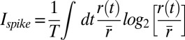, where is the average stimulus evoked firing rate and time uniquely identifies different stimuli within the segment of duration T that was repeated multiple times. Sparseness of the neural firing rate was quantified as normalized variance of the PSTH : 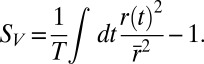This quantity is monotonically related to previous measures of sparseness (47) , although it is not limited to be between 0 and 1. Just as information provides an upper bound for the amount of information that can be accounted for by a model of reduced dimensionality, this measure of sparseness provides an upper bound for the amount of variance that can be accounted for by such models (48).

Threshold Estimation.

To estimate a threshold value for each neuron, we examined how its firing rate was modulated by the value of stimulus component along MIID1 (evaluated at the most likely spatial position to have elicited a spike within a given stimulus frame). The smallest value of stimulus component along MIID1 where the firing rate was significantly different (P < 0.05) from the mean stimulus-evoked firing rate was taken as the estimate of spiking threshold.

Inclusion Criteria.

We recorded from 161 single units in two animals. When evaluating predictive power of estimated models, we excluded those cells where the overall information about visual stimuli carried by single spikes was not significantly different from zero (P > 0.05) or less than 0.1 bits. We also compared the values of the mutual information computed with and without linear extrapolation to the infinite dataset size. Those cells where these two values were significantly different (P < 0.05) were also excluded. The latter criterion eliminates cells where the overall information value changed strongly with a small expansion of the dataset, which suggests that the dataset for that neuron was not large enough to ensure a reliable extrapolation to the infinite dataset size. The same criteria were applied to LN models with different ranges of position invariance fitted to responses of each neuron, that is, models that provided predictions that were not significantly different from zero or strongly dependent on the size of the dataset were excluded from subsequent analyses. The threshold for statistical significance was modified according to Sidak correction to take into account that multiple models with different ranges of position invariance were tested. LN models satisfying these criteria were obtained for 109 neurons out of 161 neurons. Measurements of the overall information carried in the neural responses were available in 38 neurons (sufficient repeated data were not available for all 161 cells).

Curved Gabor Models.

To quantify curvature selectivity, we fit the measured profiles of relevant features using a curved Gabor model defined as 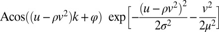. Here, parameter describes the orientation of the contour, with variables and describing the rotation from horizontal x and vertical y directions. Other parameters stand for amplitude A, curvature , spatial phase , spatial frequency k, the width , and the length of the contour. When the curvature parameter is set to zero this model reduces to the classic Gabor model (49) that can produce localized bars and edges. The criteria for successful fitting of curved Gabor models were that the correlation coefficient between the measured and fitted profiles was >0.6. In addition, we required parameters (in units of frame size), and . The later criteria are designed to exclude unreasonably high estimates of receptive field sizes that grossly exceed the frame size or of curvatures that cannot be resolved given the “width” of the contour. The largest ratio of observed among well-fit receptive fields was ∼20. This corresponds to the circumference of the osculating circle 2 > 0.3 L, where L is the wavelength of the oscillation defined by the spatial frequency. Larger values of curvatures just appear as a blob. Fitting of relevant stimulus features of model cells was always successful according to these criteria, yielding correlation coefficients >0.8. In the case of real data, out of 109 neurons this fitting was successful in 38 neurons for either the first or the second relevant dimension and in 18 neurons for both features. We note that it is more difficult to fit receptive fields with very sharp curvatures. Although the fitting procedure itself is independent of the degree of position invariance, because higher curvatures are associated with smaller position invariance (Fig. 1D) the quality of a fit to cells’ receptive fields with a curved Gabor model (as measured by correlation coefficient) decreased with position invariance (P = 0.01 for MIID1). The effect is most pronounced for neurons with zero degree of position invariance. Here, we could successfully fit both features in only 8% of position-specific neurons, compared with ∼30% of neurons with partial position invariance within the range of 5–15%. Many of the neurons with position-specific receptive fields are likely to be corner detectors, but at present it was not clear how to quantitatively characterize their receptive fields given uncertainties in the receptive field estimation. Therefore, we limited the study of the trade-off between curvature and invariance to cells with finite (nonzero) position invariance, because within this range of position invariance similar fractions of cells’ receptive fields were well fitted with the curved Gabor model.

References

- 1.DiCarlo JJ, Zoccolan D, Rust NC. How does the brain solve visual object recognition? Neuron. 2012;73(3):415–434. doi: 10.1016/j.neuron.2012.01.010. [DOI] [PMC free article] [PubMed] [Google Scholar]
- 2.Serre T, Wolf L, Bileschi S, Riesenhuber M, Poggio T. Robust object recognition with cortex-like mechanisms. IEEE Trans Pattern Anal Mach Intell. 2007;29(3):411–426. doi: 10.1109/TPAMI.2007.56. [DOI] [PubMed] [Google Scholar]
- 3.Rust NC, Dicarlo JJ. Selectivity and tolerance (“invariance”) both increase as visual information propagates from cortical area V4 to IT. J Neurosci. 2010;30(39):12978–12995. doi: 10.1523/JNEUROSCI.0179-10.2010. [DOI] [PMC free article] [PubMed] [Google Scholar]
- 4.Hubel DH, Wiesel TN. Receptive fields and functional architecture of monkey striate cortex. J Physiol. 1968;195(1):215–243. doi: 10.1113/jphysiol.1968.sp008455. [DOI] [PMC free article] [PubMed] [Google Scholar]
- 5.McManus JN, Li W, Gilbert CD. Adaptive shape processing in primary visual cortex. Proc Natl Acad Sci USA. 2011;108(24):9739–9746. doi: 10.1073/pnas.1105855108. [DOI] [PMC free article] [PubMed] [Google Scholar]
- 6.Anzai A, Peng X, Van Essen DC. Neurons in monkey visual area V2 encode combinations of orientations. Nat Neurosci. 2007;10(10):1313–1321. doi: 10.1038/nn1975. [DOI] [PubMed] [Google Scholar]
- 7.Kourtzi Z, Connor CE. Neural representations for object perception: Structure, category, and adaptive coding. Annu Rev Neurosci. 2011;34:45–67. doi: 10.1146/annurev-neuro-060909-153218. [DOI] [PubMed] [Google Scholar]
- 8.Roe AW, et al. Toward a unified theory of visual area V4. Neuron. 2012;74(1):12–29. doi: 10.1016/j.neuron.2012.03.011. [DOI] [PMC free article] [PubMed] [Google Scholar]
- 9.Gallant JL, Connor CE, Rakshit S, Lewis JW, Van Essen DC. Neural responses to polar, hyperbolic, and Cartesian gratings in area V4 of the macaque monkey. J Neurophysiol. 1996;76(4):2718–2739. doi: 10.1152/jn.1996.76.4.2718. [DOI] [PubMed] [Google Scholar]
- 10.Zoccolan D, Kouh M, Poggio T, DiCarlo JJ. Trade-off between object selectivity and tolerance in monkey inferotemporal cortex. J Neurosci. 2007;27(45):12292–12307. doi: 10.1523/JNEUROSCI.1897-07.2007. [DOI] [PMC free article] [PubMed] [Google Scholar]
- 11.Gawne TJ, Martin JM. Responses of primate visual cortical V4 neurons to simultaneously presented stimuli. J Neurophysiol. 2002;88(3):1128–1135. doi: 10.1152/jn.2002.88.3.1128. [DOI] [PubMed] [Google Scholar]
- 12.Johnson JS, Olshausen BA. The recognition of partially visible natural objects in the presence and absence of their occluders. Vision Res. 2005;45(25-26):3262–3276. doi: 10.1016/j.visres.2005.06.007. [DOI] [PubMed] [Google Scholar]
- 13.Gross CG. Genealogy of the “grandmother cell.”. Neuroscientist. 2002;8(5):512–518. doi: 10.1177/107385802237175. [DOI] [PubMed] [Google Scholar]
- 14.Quiroga RQ. Concept cells: The building blocks of declarative memory functions. Nat Rev Neurosci. 2012;13(8):587–597. doi: 10.1038/nrn3251. [DOI] [PubMed] [Google Scholar]
- 15. Bouvrie J, Rosasco L, Poggio T (2009) On invariance in hierarchical models. Advances in Neural Information Processing Systems 22, eds. Bengio Y, Schuurmans D, Lafferty J, Williams CKI, Culotta A (Neural Information Processing Systems Foundation, La Jolla, CA), pp 162–170.
- 16.Ullman S, Soloviev S. Computation of pattern invariance in brain-like structures. Neural Netw. 1999;12(7-8):1021–1036. doi: 10.1016/s0893-6080(99)00048-9. [DOI] [PubMed] [Google Scholar]
- 17.Pasupathy A, Connor CE. Population coding of shape in area V4. Nat Neurosci. 2002;5(12):1332–1338. doi: 10.1038/nn972. [DOI] [PubMed] [Google Scholar]
- 18.Connor CE, Brincat SL, Pasupathy A. Transformation of shape information in the ventral pathway. Curr Opin Neurobiol. 2007;17(2):140–147. doi: 10.1016/j.conb.2007.03.002. [DOI] [PubMed] [Google Scholar]
- 19.Pasupathy A, Connor CE. Responses to contour features in macaque area V4. J Neurophysiol. 1999;82(5):2490–2502. doi: 10.1152/jn.1999.82.5.2490. [DOI] [PubMed] [Google Scholar]
- 20.David SV, Hayden BY, Gallant JL. Spectral receptive field properties explain shape selectivity in area V4. J Neurophysiol. 2006;96(6):3492–3505. doi: 10.1152/jn.00575.2006. [DOI] [PubMed] [Google Scholar]
- 21.Eickenberg M, Rowekamp RJ, Kouh M, Sharpee TO. Characterizing responses of translation-invariant neurons to natural stimuli: Maximally informative invariant dimensions. Neural Comput. 2012;24(9):2384–2421. doi: 10.1162/NECO_a_00330. [DOI] [PMC free article] [PubMed] [Google Scholar]
- 22.Meister M, Berry MJ., 2nd The neural code of the retina. Neuron. 1999;22(3):435–450. doi: 10.1016/s0896-6273(00)80700-x. [DOI] [PubMed] [Google Scholar]
- 23.Victor J, Shapley R. A method of nonlinear analysis in the frequency domain. Biophys J. 1980;29(3):459–483. doi: 10.1016/S0006-3495(80)85146-0. [DOI] [PMC free article] [PubMed] [Google Scholar]
- 24.Rust NC, Schwartz O, Movshon JA, Simoncelli EP. Spatiotemporal elements of macaque v1 receptive fields. Neuron. 2005;46(6):945–956. doi: 10.1016/j.neuron.2005.05.021. [DOI] [PubMed] [Google Scholar]
- 25.Schwartz O, Pillow JW, Rust NC, Simoncelli EP. Spike-triggered neural characterization. J Vis. 2006;6(4):484–507. doi: 10.1167/6.4.13. [DOI] [PubMed] [Google Scholar]
- 26.Touryan J, Lau B, Dan Y. Isolation of relevant visual features from random stimuli for cortical complex cells. J Neurosci. 2002;22(24):10811–10818. doi: 10.1523/JNEUROSCI.22-24-10811.2002. [DOI] [PMC free article] [PubMed] [Google Scholar]
- 27.de Ruyter van Steveninck RR, Bialek W. Real-time performance of a movement-sensitive neuron in the blowfly visual system: Coding and information transfer in short spike sequences. Proc R Soc Lond B Biol Sci. 1988;234:379–414. [Google Scholar]
- 28. Bialek W, de Ruyter van Steveninck RR (2005) Features and dimensions: Motion estimation in fly vision, arXiv:q-bio/0505003.
- 29.Hubel DH, Wiesel TN. Receptive fields and functional architecture in two nonstriate visual areas (18 and 19) of the cat. J Neurophysiol. 1965;28:229–289. doi: 10.1152/jn.1965.28.2.229. [DOI] [PubMed] [Google Scholar]
- 30.Riesenhuber M, Poggio T. Hierarchical models of object recognition in cortex. Nat Neurosci. 1999;2(11):1019–1025. doi: 10.1038/14819. [DOI] [PubMed] [Google Scholar]
- 31.Shadlen MN, Movshon JA. Synchrony unbound: A critical evaluation of the temporal binding hypothesis. Neuron. 1999;24(1):67–77, 111–125. doi: 10.1016/s0896-6273(00)80822-3. [DOI] [PubMed] [Google Scholar]
- 32.DeAngelis GC, Ghose GM, Ohzawa I, Freeman RD. Functional micro-organization of primary visual cortex: Receptive field analysis of nearby neurons. J Neurosci. 1999;19(10):4046–4064. doi: 10.1523/JNEUROSCI.19-10-04046.1999. [DOI] [PMC free article] [PubMed] [Google Scholar]
- 33.de Boer R, Kuyper P. Triggered correlation. IEEE Trans Biomed Eng. 1968;15(3):169–179. doi: 10.1109/tbme.1968.4502561. [DOI] [PubMed] [Google Scholar]
- 34.Sharpee T, Rust NC, Bialek W. Analyzing neural responses to natural signals: maximally informative dimensions. Neural Comput. 2004;16(2):223–250. doi: 10.1162/089976604322742010. [DOI] [PubMed] [Google Scholar]
- 35.Adelson EH, Bergen JR. Spatiotemporal energy models for the perception of motion. J Opt Soc Am A. 1985;2(2):284–299. doi: 10.1364/josaa.2.000284. [DOI] [PubMed] [Google Scholar]
- 36.Dobbins A, Zucker SW, Cynader MS. Endstopped neurons in the visual cortex as a substrate for calculating curvature. Nature. 1987;329(6138):438–441. doi: 10.1038/329438a0. [DOI] [PubMed] [Google Scholar]
- 37.Ben-Shahar O, Zucker S. Geometrical computations explain projection patterns of long-range horizontal connections in visual cortex. Neural Comput. 2004;16(3):445–476. doi: 10.1162/089976604772744866. [DOI] [PubMed] [Google Scholar]
- 38.Kouh M, Sharpee TO. Estimating linear-nonlinear models using Renyi divergences. Network. 2009;20(2):49–68. doi: 10.1080/09548980902950891. [DOI] [PMC free article] [PubMed] [Google Scholar]
- 39.Sharpee TO, et al. Adaptive filtering enhances information transmission in visual cortex. Nature. 2006;439(7079):936–942. doi: 10.1038/nature04519. [DOI] [PMC free article] [PubMed] [Google Scholar]
- 40.Cadieu C, et al. A model of V4 shape selectivity and invariance. J Neurophysiol. 2007;98(3):1733–1750. doi: 10.1152/jn.01265.2006. [DOI] [PubMed] [Google Scholar]
- 41.Pasupathy A, Connor CE. Shape representation in area V4: Position-specific tuning for boundary conformation. J Neurophysiol. 2001;86(5):2505–2519. doi: 10.1152/jn.2001.86.5.2505. [DOI] [PubMed] [Google Scholar]
- 42.Kunsberg B, Zucker SW. Shape-from-shading and cortical computation: A new formulation. J Vis. 2012;12(9):233. [Google Scholar]
- 43.Lehky SR, Sejnowski TJ. Network model of shape-from-shading: neural function arises from both receptive and projective fields. Nature. 1988;333(6172):452–454. doi: 10.1038/333452a0. [DOI] [PubMed] [Google Scholar]
- 44.Motter BC. Central V4 receptive fields are scaled by the V1 cortical magnification and correspond to a constant-sized sampling of the V1 surface. J Neurosci. 2009;29(18):5749–5757. doi: 10.1523/JNEUROSCI.4496-08.2009. [DOI] [PMC free article] [PubMed] [Google Scholar]
- 45.Reynolds JH, Chelazzi L, Desimone R. Competitive mechanisms subserve attention in macaque areas V2 and V4. J Neurosci. 1999;19(5):1736–1753. doi: 10.1523/JNEUROSCI.19-05-01736.1999. [DOI] [PMC free article] [PubMed] [Google Scholar]
- 46.Brenner N, Strong SP, Koberle R, Bialek W, de Ruyter van Steveninck RR. Synergy in a neural code. Neural Comput. 2000;12(7):1531–1552. doi: 10.1162/089976600300015259. [DOI] [PubMed] [Google Scholar]
- 47.Vinje WE, Gallant JL. Sparse coding and decorrelation in primary visual cortex during natural vision. Science. 2000;287(5456):1273–1276. doi: 10.1126/science.287.5456.1273. [DOI] [PubMed] [Google Scholar]
- 48.Sharpee TO. Comparison of information and variance maximization strategies for characterizing neural feature selectivity. Stat Med. 2007;26(21):4009–4031. doi: 10.1002/sim.2931. [DOI] [PubMed] [Google Scholar]
- 49.DeAngelis GC, Ohzawa I, Freeman RD. Spatiotemporal organization of simple-cell receptive fields in the cat’s striate cortex. II. Linearity of temporal and spatial summation. J Neurophysiol. 1993;69(4):1118–1135. doi: 10.1152/jn.1993.69.4.1118. [DOI] [PubMed] [Google Scholar]
Associated Data
This section collects any data citations, data availability statements, or supplementary materials included in this article.