Dynamics of Self-assembly of Model Viral Capsids in the Presence of a Fluctuating Membrane

Abstract

A coarse-grained computational model is used to investigate the effect of a fluctuating fluid membrane on the dynamics of patchy-particle assembly into virus capsid-like cores. Results from simulations for a broad range of parameters are presented, showing the effect of varying interaction strength, membrane stiffness, and membrane viscosity. Furthermore, the effect of hydrodynamic interactions is investigated. Attraction to a membrane may promote assembly, including for subunit interaction strengths for which it does not occur in the bulk, and may also decrease single-core assembly time. The membrane budding rate is strongly increased by hydrodynamic interactions. The membrane deformation rate is important in determining the finite-time yield. Higher rates may decrease the entropic penalty for assembly and help guide subunits toward each other but may also block partial cores from being completed. For increasing subunit interaction strength, three regimes with different effects of the membrane are identified.

1. Introduction

The formation of the protein shell of viruses has, due to its relative simplicity and importance in many diseases, become one of the most well-studied examples of self-assembly.¹ Although viruses are typically assembled within the cells of their host, the process may also be triggered in a bulk solution of viral proteins by changing the pH.² Such experiments have stimulated the application of simple computational models^1,3−7 to help understand assembly processes.

While much modeling has focused on the formation of virus capsids in the bulk, in recent work investigating the growth of viral shells around their genome, the assembly of simple subunits attracted to a flexible polymer was simulated.^8,9 Interaction with the polymer was found to allow assembly for parameters for which it would otherwise not occur. Encapsulation of spherical nanoparticles has also been considered both in experiment¹⁰ and in simulation.^11,12 Experimentally, it was demonstrated that shells resembling different types of viral particles could be assembled by varying the nanoparticle diameter.

Beyond interactions with an encapsulated genome, there is also much evidence that membranes play an important role in assembly for many viruses.¹³⁻²¹ In a recent publication,²² we presented results on the effect of fluctuating membranes on the equilibrium of a system of self-assembling patchy colloids, designed to assemble viral core-like structures, from Monte Carlo (MC) simulations.²³ We found a nonmonotonic dependence of the promotion of assembly on membrane stiffness, as well as the formation of membrane buds. It is of course true that such effects would be observable in an analogous experimental system after sufficient time and to be expected that they will influence the products of dynamical assembly. However, on relevant time scales, self-assembly processes may not reach equilibrium and the products may be affected, for example, by kinetic traps.^1,24 It is therefore of foremost interest to consider simulations with realistic dynamics. Key dynamical features that we capture in our simulations are the viscosity of the membrane and hydrodynamic interactions, the inclusion of which may alter dynamics both quantitatively and qualitatively.²⁵

Two key factors in the present work are attractions to the fluctuating membrane and hydrodynamic interactions. Previous computational studies have looked into the effects of each of these individually on the clusters formed by isotropic spherical colloids. Hydrodynamic interactions were found to change both the size and shape of clusters,²⁶ while attraction to a membrane was found to induce the formation of linear chains on the surface.²⁷ Further, attractions of particles to a membrane surface may cause the formation of buds^22,28,29 or tube-like structures.^30,31

Here, as a simple model to gain insight into the effect of membranes on the dynamics of self-assembly, we consider primarily the same, patchy-particle, subunits,^6,32 which may assemble 12-component cores, as in our previous work,²² and simulate their assembly using a dynamically realistic method. As previously, our subunits are coupled to a membrane modeled using particles bonded to form a triangulated surface.^33,34 The target core structure has icosahedral symmetry, similar to many viruses, although in reality enveloped viruses are larger. The remainder of the paper is organized as follows. In section 2 we describe our simulation models and in section 3 we present results from MC simulations on the equilibrium of the system. We then move on to dynamical simulations, describing simulation methods in section 4. We present results for the 12-component cores in section 5 and compare them to some results for other cores in section 6. Finally, we conclude in section 7.

2. Simulation Models

Rather than only considering enough subunits to form just one target structure as in our previous work,²² we now simulate 180, allowing a maximum of 15 complete cores to be assembled. While it is expected that in experimental and biological situations it is also likely that a larger number of subunits will be available than required for one complete structure, this choice was additionally made for computational efficiency, so that, on a feasible time scale, although assembly of all possible cores may not occur, some complete cores will form. We simulate a membrane composed of 1156 particles. The simulation setup is sketched in Figure 1a.

Figure 1.

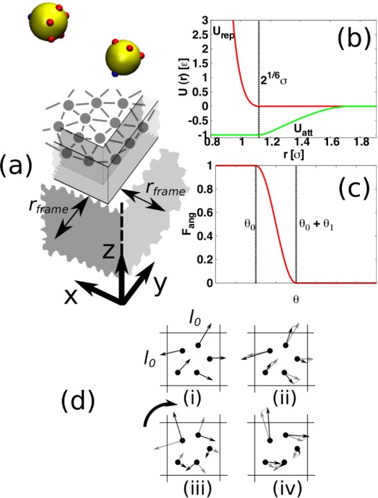
(a) Simulation setup. Subunits, which are all identical, are rendered in yellow, with positions, but not extents, of patches for interactions with other subunits in red. Positions of patches for interactions with the membrane particles are in blue. The membrane is modeled as a triangulated surface of bonded particles. The particles forming the surface edge are confined to a frame region, which is located at a distance r_frame from the periodic boundaries. In simulations with hydrodynamics, a stochastic rotation dynamics (SRD) solvent composed of point particles is included. Interactions between SRD particles are effected by first dividing the entire system into a grid of cells of side l₀. (b) The radial part of the inter-subunit or subunit-membrane potential, U(r), with a well-depth ε is split into attractive (green) and repulsive parts (red). (c) The attractive part is multiplied by factors of the form F_ang(θ), where θ is an angle that depends on the relative orientation of the interacting particles. (d) Sketch of momentum transfer between SRD particles in a cell: (i) Only particles within one cell interact. (ii) Velocities are subtracted from all particles such that the center of mass velocity is 0. (iii) All velocities are rotated, as signified by the heavy arrow, around a random axis, by a given angle. (iv) The subtracted velocities are added back on so that total momentum is conserved.

The interactions between subunits, ss, and between subunits and membrane particles, ms, are identical to those used in our previous work²² but we describe the important features again here. The potentials are based on a Lennard-Jones form. As shown in eq 1, the potential is split into attractive, U_att, and repulsive, U_rep, parts. The interaction of two particles, i and j, separated by r_ij (i ≠ j), with orientations Ω_i and Ω_j, either both subunits or a subunit and a membrane particle, is given by

1

where the forms of U_att and U_rep are shown in Figure 1b. γ_area, γ_att and γ_orient are dimensionless factors that take different forms for ss and ms interactions. For ss-interactions, γ_area = γ_att = 1 and, as depicted in Figure 1a, there are 5 patches on each subunit, which are arranged symmetrically around a single ms patch. The minimum of U_att is set to −ε_ss. γ_orient is used to control the patch width, and it has the form of a product of three functions of the form shown in Figure 1c, see also the Supporting Information. For the first two factors, the argument is the angle between the interacting patches and the center-to-center vector, r_ij. The parameters for determining patch width, see Figure 1c, are set to θ₀ = θ₁ = 0.2. In contrast, for the third factor, the argument is the angle between the projections of the membrane patches onto the plane perpendicular to r_ij and θ₀ = θ₁ = 0.4. The third factor represents the torsional stiffness of protein interactions.⁶

For ms-interactions, the minimum of U_att is set to −ε_ms. In these interactions, only the subunits are patchy, having one patch. Parameters for the one orientational function composing γ_orient, see Figure 1c, are θ₀ = π/4 and θ₁ = 0.2, and there is no penalty for subunits rotating around r_ij. Since, typically, assembling proteins will only be able to access one side of a membrane, we choose to make only one side of the membrane in our simulations attractive to subunits.³⁵ This is achieved by setting γ_att = 1 if a subunit interacts with the “upper” side and γ_att = 0 if it interacts with the “lower” side. The γ_area factor is proportional to the area of surface that surrounds the interacting membrane particle. The length scale for ss-interactions is chosen as σ_ss = 2.5l₀ and the length scale for ms interactions is σ_ms = 1.75l₀, where l₀ is a simulation unit of length. For the exact functional forms used in the ss and ms interactions, see the Supporting Information.

The membrane is modeled as in ref.³⁵ but we describe the key features again here. As depicted in Figure 1a, the membrane is composed of particles bonded to form a triangulated surface. To include membrane fluidity, MC moves that flip bonds between different particles are included.³⁴ The typical separation between bonded membrane particles is l₀, maintained by a potential that has a flat central region but diverges at 0.67l₀ and 1.33l₀, see Supporting Information. We perform simulations in a box of size 45l₀ × 45l₀ × 45l₀, giving a subunit number density within the range for which yield was found to weakly depend on concentration.⁶ As in our previous work,²² we consider a range of ε_ss that, at equilibrium in the bulk, covers the crossover to complete assembly of all cores. Although approximately centered around the same ε_ss value, for the larger number of cores considered here, the crossover is broader³⁶ and so a wider range of ε_ss is used. The same range of ε_ms as in ref (22) is considered, chosen to cover the crossover from freely diffusing to membrane-bound structures. The stiffness of our membrane is controlled by a parameter λ_b, through a potential, U_bend = λ_b(1 – n_i·n_j), applied to all pairs of neighboring triangles in the surface, where n_i and n_j are the unit normal vectors of the triangles. We simulate using the three middle values from our previous work,²² λ_b = √3k_BT, 2√3k_BT and 4√3k_BT: at equilibrium, this covers the crossover from cores being able to cause budding of the membrane to them not being able to. As discussed in our previous work,²² this range of bending stiffness is at the lower end of that expected for biological membranes. Given that in viral budding³⁷ intrinsic curvature is expected to be important, which is neglected in our model, the bending stiffness in our simulation is most relevant in terms of the cost of deformation.

Although our focus is on dynamical simulation, we first investigate the equilibrium of the system for comparison. For this purpose, we use MC simulations, employing a similar approach as in our previous work.²² On the other hand, for molecular dynamics (MD) simulations, we include hydrodynamic interactions using a stochastic rotation dynamics (SRD) solvent,³⁸ a coarse-grained method in which the fluid is represented by point particles. SRD particle interactions are effected by dividing the system into a grid of cells, of side l₀, at regular intervals and exchanging momentum by a rotation through a certain angle of velocities relative to the cell center of mass velocity. This procedure is shown schematically in Figure 1d. To understand the influence of hydrodynamic interactions, we also simulate using a method that neglects them, Langevin dynamics (LD), in which the effect of the solvent is represented by uncorrelated random, as well as drag, forces.^39,40

To simulate a tensionless membrane, rather than box rescaling,²² we use a new membrane boundary condition, recently introduced by us,³⁵ which is compatible with SRD. The edge of the membrane is attached to a square frame, with sides positioned at a distance r_frame into the simulation box, as depicted in Figure 1a. For those triangles in the surface that have a side that forms part of the membrane edge, a bending potential of the same form as that between neighboring triangles is applied, except that the unit normal of the triangle is compared to a unit normal to the frame-plane. The distance r_frame may increase and decrease during the simulation. To allow for deformation, the number of membrane particles bonded to the frame may also vary, with corresponding changes to the number of bonds in the bulk of the surface, N_b–bulk. For more details of the membrane boundary condition, see the appendix of ref (35), the functional form of the confining potential is also given in the Supporting Information. For consistency, this approach is also used in MC and LD simulations, in which, of course, the solvent is absent.

3. Results from Equilibrium Simulations

We first present, in Figure 2, results from MC simulations on the yield of complete cores, defined to be a cluster of 12 bonded subunits, each unit making 5 bonds to other cluster members. Two subunits are defined to be bonded if their interaction energy is < −0.25ε_ss. Interaction strengths for different simulations lie on a grid from 0.12 to k_BT in spacings of 0.08k_BT for ε_ms and from 4.5 to 8.02k_BT in spacings of 0.32k_BT for ε_ss. Systems at different parameters were run in parallel using Multicanonical Parallel Tempering.⁴¹ For each data point in Figure 2, approximately 4 × 10⁹ attempted MC moves were performed, including about 4 × 10⁴ Hybrid MC moves,⁴² as well as Aggregate Volume Bias moves.⁴³ These were both found to significantly speed up relaxation. The largest error for a single data point was estimated to be about 0.6. Similarly to our results with one core,²² for λ_b = √3k_BT and λ_b = 2√3k_BT at higher ε_ms, the assembly of the cores causes the membrane to form buds, although these now generally contain multiple cores. For λ_b = 4√3k_BT, budding did not occur. Again as for single cores, for high ε_ms, assembly occurs for lower values of ε_ss: the membrane promotes assembly. Here, membrane-dependent, low ε_ss assembly does not occur to the same extent as for high ε_ss because, due to steric repulsion, only a fraction of the cores may interact with the membrane at once, typically about 4 cores in the case where a bud is formed. Whereas for one core, the range over which promotion occurred was clearly largest for λ_b = √3k_BT, here the results for λ_b = 2√3k_BT are very similar. This may be because multiple cores together effectively form a larger object deforming the membrane.

Figure 2.

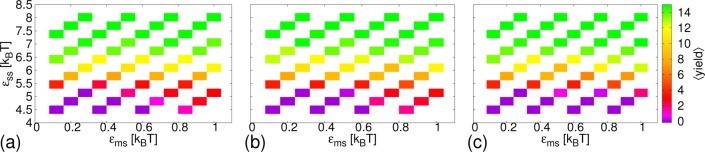
Results from MC simulations. Average yield of complete cores, ⟨yield⟩, as a function of subunit-membrane interaction strength, ε_ms, and inter-subunit interaction strength, ε_ss, for different membrane stiffnesses, λ_b: (a) λ_b = √3k_BT; (b) λ_b = 2√3k_BT; (c) λ_b = 4√3k_BT.

4. Dynamical Simulation Methods

We next give details of our dynamical simulation methods. The SRD particles have mass m and number density per cell γ = 5. We define our unit of time, t₀ = l₀(m/k_BT)^1/2. Collisions are performed every Δt_coll = 10^–1t₀ and we use an SRD rotation angle of π/2, giving a fluid viscosity of η_f = 2.5m/l₀t₀.⁴⁴ We apply a SRD-cell level thermostat that conserves momentum to maintain the temperature.³⁸ Membrane particles are coupled to the SRD solvent by including them in the collision step.³⁸ There will typically be about one membrane particle per SRD cell and we set their mass to γm, giving a short-time friction coefficient ζ_mem = 15.8(m/t₀).⁴⁴

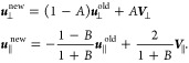
Unlike membrane particles, subunits have rotational degrees of freedom and so are coupled to the SRD solvent using bounce-back boundary conditions.⁴⁵ For their interactions with the fluid, subunits are treated as solid spherical particles of radius a = l₀, having mass M = (4/3)πa³mγ and moment of inertia I = (2/5)Ma². Every Δt_bound = 10^–2t₀, the SRD particles are checked. If an overlap with a subunit is detected, then the SRD particle with velocity u is first moved by (−1/2)Δt_boundu and then shifted radially to the edge of the subunit, r from the center, where |r| = a. This scheme is based on the fact that for SRD particles the average crossing of the subunit boundary is halfway through a time step. It was found to function well in previous work.⁴⁶ A bounce-back collision is then performed: the radial, u_⊥, and tangential, u_∥, components of u are updated according to

2

Here, A = 2M/(m+M), B = 7m/2M and the surface velocity V = v + ω × r, where v is the center of mass velocity of the subunit and ω is its angular velocity around an axis that passes through the center of mass. Equation 2 is valid for I = 2/5Ma². After all overlapping SRD particles have been rebounded, corresponding changes to the subunit velocity and angular velocity, Δv = (m/M)Σ_i(u_i^old – u_i) and Δω= (m/I)Σ_ir_i × (u_i^old – u_i), where i indexes the different rebounded particles, are applied so that momentum and energy are conserved. If M ≫ m, SRD particle velocities relative to the surface are completely reversed; for our parameters, M ≈ 20m.

Overlapping of embedded particles in an SRD fluid may lead to a spurious depletion attraction.⁴⁷ In fact, even if particles are prevented from overlapping, the bounce-back scheme may need to be iterated due to the possibility of a fluid particle interacting with more than one solute particle within Δt_bound. We avoid these issues by choosing the excluded volume length for subunit interactions, σ_ss = 2.5l₀, so that the typical closest approach of two subunit fluid surfaces ≈ 0.5l₀ is much greater than the typical displacement of a fluid particle ≈ 10^–2l₀.

Bounce-back interactions between SRD particles and embedded colloids lead to spurious slips at the colloid surface. Methods exist to ameliorate this by the introduction of virtual particles but, for mobile colloids, this was found to lead to deviations from expected thermal distributions.⁴⁵ In our simulations, the concern is moot anyway, because of the discrepancy between the radii chosen for inter-subunit and subunit-fluid interactions. Effectively, there is a slip-velocity at the subunit surface, as defined by its interactions with other subunits, which has contributions from these two different sources. Given that the subunits are typically representing protein complexes, which are rough on length-scales up to many solvent molecules,⁴⁸ rather than smooth colloids, this is reasonable.

For bounce-back boundaries, the short-time friction coefficients for the subunits may be calculated using a modified Enskog theory.⁴⁵ For our parameter choice, this gives coefficients of ζ_v = 62.0(m/t₀) and ζ_ω = 73.3(ml₀²/t₀), for linear and angular velocities respectively. Comparing the corresponding correlation times, M/ζ_v and I/ζ_ω, to typical thermal velocities, we obtain values of 0.07l₀ and 0.04 for the typical length and angular displacements over which the subunit motion is correlated. These are smaller than the typical separation of subunits and patches, given by σ_ss = 2.5l₀ and ≈ 0.4 respectively, so that at the scale that assembly occurs on, subunit motion is diffusive. Similarly, the length scale over which membrane particle motion is correlated is 0.1l₀.

To obtain parameters for simulations without hydrodynamic interactions, we simulated single subunits and membrane particles in a box of the same size as that used for assembly with an SRD solvent. The friction coefficients extracted were lower than the short-time values due to long-time hydrodynamic contributions. These friction coefficients were input to LD simulations. In this way, the hydrodynamic contribution to the self-diffusion coefficients is included but hydrodynamic interactions between different particles are neglected. An alternative approach to simulating without hydrodynamics is to use an SRD fluid and randomize particle velocities at every step. For colloids, however, this has been found to introduce an unphysical caging effect.⁴⁹

Membrane fluidity is included by performing a certain number of attempts to flip bonds between neighboring pairs of membrane particles³⁴ every 10^–1t₀. The membrane viscosity is set by the level of attempted bond-flips and we consider three different rates: N_b–bulk, 10^–1N_b–bulk and 10^–2N_b–bulk attempted bond-flips per 10^–1t₀, where N_b–bulk is the number of bonds in the bulk of the membrane and the resulting numbers are rounded to integers. By considering Poiseuille flows in two-dimensional membranes,³⁴ the corresponding membrane viscosity, η_m, may be estimated. For the highest rate of flips the value is estimated to be 35.1 ± 0.1m/t₀,³⁵ whereas for the lower rates we estimate 133.3 ± 0.6m/t₀ and 1190 ± 60m/t₀ respectively. For a lipid bilayer in water, the ratio of membrane to fluid viscosities, l_η, is typically around 1–10 μm.⁵⁰ In our simulations the solvent viscosity η_f = 2.5m/l₀t₀ so that, if our subunits represent capsomers with a size on the order of 10 nm,⁵¹ then the ratio of their hydrodynamic radius to l_η is around the expected range.

5. Results from Dynamical Simulations

We next present results from our dynamical simulations. Interaction strengths for dynamical simulations were chosen to coincide with those for MC simulations, although fewer were considered due to higher computational costs. A closer spacing between the highest interaction strengths was chosen as it was expected that the most interesting results would be found here. All averages are taken over at least 5 independent runs and in some cases over 10. We consider the same values of λ_b, and also ε_ms and ε_ss in the same range, as for the equilibrium MC simulations. We simulate primarily using SRD but, for λ_b = √3k_BT and 2√3k_BT, we also simulate using LD for comparison, to gain insight into the importance of hydrodynamic interactions. LD simulations were essentially identical to the SRD ones expect that, rather than having regular interactions with an explicit fluid, subunits and membrane particles were, at each MD integration step, subject to random and friction forces.^39,40 The system was initially simulated for either 8 × 10³t₀ with SRD, or 2 × 10⁴t₀ with LD, without attractive interactions. These times were chosen as being sufficient to allow membrane relaxation. Subsequently, attractions were switched on and the system was simulated for a further 5 × 10⁴t₀ to gather results. In contrast to the MC results, for the stiffest membrane, λ_b = 4√3k_BT, with the highest membrane-subunit interaction strength only, ε_ms = k_BT, in some, though not all runs, budding occurred.

Were it possible to run the dynamical simulations indefinitely, it is expected that results would eventually converge to those found for the equilibrium simulations. However, as the simulation progresses, further assembly becomes increasing slow as the supply of free subunits is depleted and eventually relies on rearrangement of subunits between partially formed structures, possibly moving into or out of a membrane bud. It is thus necessary to choose a finite simulation time shorter than that required for complete assembly and inevitably the results obtained will depend on it. For our chosen simulation time, the highest yield observed in any simulation is ∼50% of the possible maximum. It is nonetheless sufficient for the effect of the membrane on assembly to be apparent. However, the finite time chosen should be borne in mind when considering the results.

First, in Figure 3, we plot the averages of various quantities as a function of ε_ms and ε_ss at different simulation times, t, for λ_b = 2√3k_BT and η_m = 133.3m/t₀. Considering Figure 3a, at later times, the largest number of correctly assembled cores are obtained for the second highest ε_ss, 7.38k_BT. This is close to the optimal value obtained in previous work⁶ with a very similar model of about 7.14k_BT. Although for the highest value, ε_ss = 8.02k_BT, the total interaction energy between subunits relative to the interaction strength is somewhat lower, see Figure 3b, this corresponds to many incomplete cores assembling, thus starving the system of free subunits. This kinetic trap is not related to the membrane and has often been observed previously.¹ In contrast, for high ε_ss, increasing attraction to the membrane hinders complete assembly due to the membrane enveloping, or partly surrounding, partial cores too quickly, thus preventing subunits or other partial cores from approaching them. The fast envelopment is apparent in Figure 3, where it may be seen that, for high ε_ms and ε_ss, the interaction energy of the subunits with the membrane approaches its final value much more quickly than the yield. Similarly to the MC results, a promotion of the finite-time assembly for low ε_ss at high ε_ms occurs.

Figure 3.

Plots as a function of subunit-membrane interaction strength, ε_ms, and inter-subunit interaction strength, ε_ss at different times, t, increasing from left to right in intervals of 1 × 10⁴t₀, for membrane stiffness, λ_b = 2√3k_BT and membrane viscosity η_m = 133.3m/t₀, from SRD simulations. (a) Average yield of complete cores, ⟨yield⟩. (b) Average total interaction energy between subunits, relative to the interaction strength, ⟨U_ss/ε_ss⟩. (c) Average total interaction energy between subunits and the membrane, relative to the interaction strength, ⟨U_ms/ε_ms⟩.

Comparing results for equilibrium, Figure 2, to those from dynamical simulations, there are several differences. Clearly, for equilibrium results, kinetic traps do not play a role. Furthermore, the interaction strength at which assembly starts is slightly lower at equilibrium than after a finite time in dynamical simulation. For the lowest ε_ms, ε_ms = 0.12k_BT, where the membrane does not play a significant role and assembly occurs in the bulk, whereas at equilibrium there are complete cores at ε_ss = 5.46k_BT, albeit at a relatively small yield, no complete cores were formed within the allowed time in dynamical simulations. Similarly, the range of parameters for which there is assembly promotion is larger for the equilibrium results.

Considering Figure 3a, we note that a time lag before complete cores are assembled, seen in previous work,¹ is apparent for many data points at t = 10⁴t₀, including for ε_ss = 7.38k_BT and low ε_ms, where the yield is highest at later times. However, for some data points, primarily with high ε_ms, some complete cores are already present at t = 10⁴t₀: as well as causing a higher yield for low ε_ss once assembly has progressed significantly, attraction to the membrane may also speed up the formation of a single core. By confining subunits to a surface, the effective size of the space that they must search to find each other is reduced. The membrane may also mediate effective attractions, directing subunits and partial cores toward each other²⁸ and, if deformation occurs, it may bring membrane-attached subunits closer together. Conversely, deformation of the membrane may also tend to block assembly, preventing partial cores from being accessed by subunits or other partial cores, leading to an increase in assembly time. The effect of the membrane on single-core assembly times is also shown in Figure 4, where we plot the average time until the first complete core in the system is formed, which we denote ⟨τ⟩, as a function of ε_ms. We note that, since this quantity is based on a single assembly event, large fluctuations were seen for lower interaction strengths and for some parameters additional simulations were run. For both membrane stiffnesses shown, λ_b = 2√3k_BT and 4√3k_BT, ⟨τ⟩ tends to be lower for high ε_ms for ε_ss = 6.42k_BT, whereas for ε_ss = 7.38k_BT the curve is flatter. For subunit interaction strengths that are approximately optimal for bulk assembly, the process is sufficiently fast that the membrane does not affect ⟨τ⟩, whereas for lower values it may cause a significant speed-up. However, we note that, for high ε_ms with some parameters, ⟨τ⟩ shows an increase. This is consistent with the membrane blocking assembly.

Figure 4.

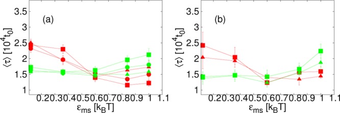
Average time until the first complete core is assembled, ⟨τ⟩, as a function of membrane-subunit interaction strength, ε_ms, for inter-subunit interaction strength, ε_ss = 6.42k_BT (red) and ε_ss = 7.38k_BT (green), with different membrane viscosities: η_m = 35.1m/t₀ (▲); η_m = 133.3m/t₀ (●); η_m = 1190m/t₀ (■). (a) Membrane stiffness, λ_b = 2√3k_BT. (b) λ_b = 4√3k_BT.

We next consider the average yield of complete cores, ⟨yield⟩, measured at the end of the simulation, at time t = 5 × 10⁴t₀. We present results for all the different parameter sets we have simulated, except for the lowest ε_ss, for which only a very small amount of assembly occurred at the highest ε_ms. We split the results into 3 figures by membrane stiffness: λ_b = √3k_BT in Figure 5; λ_b = 2√3k_BT in Figure 6; λ_b = 4√3k_BT in Figure 7. Within each figure, results are divided by ε_ss into four different subfigures labeled a–d. ⟨yield⟩ is plotted as a function of ε_ms, with curves corresponding to different membrane viscosities and simulation methods indicated by different colors, symbols and line types. Rather than describe in detail the specific features of each figure, we discuss the general trends that arise and pick out interesting features.

Figure 5.

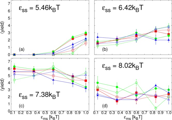
Plots of the average yield of complete cores, ⟨yield⟩, as a function of membrane-subunit interaction strength, ε_ms, for membrane stiffness, λ_b = √3k_BT at t = 5 × 10⁴t₀. From simulations with SRD (solid lines, filled symbols) or LD (dashed lines, open symbols), for different membrane viscosities: η_m = 35.1m/t₀ (blue, ▲/Δ); η_m = 133.3m/t₀ (green, ●/○); η_m = 1190m/t₀ (red, ■/□); and subunit interaction strengths, ε_ss, as indicated in panels a–d.

Figure 6.

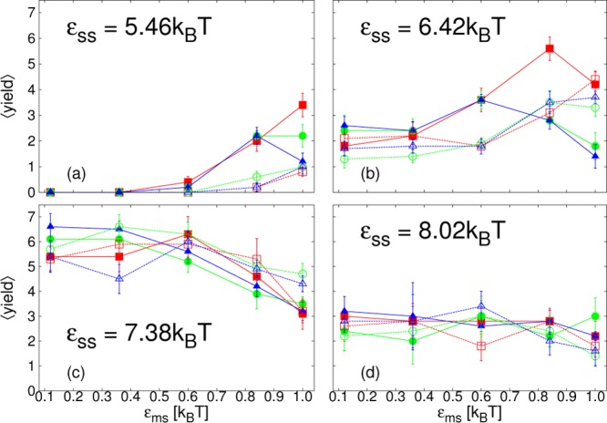
Plots of the average yield of complete cores, ⟨yield⟩, as a function of membrane-subunit interaction strength, ε_ms, for membrane stiffness, λ_b = 2√3k_BT at t = 5 × 10⁴t₀. From simulations with SRD (solid lines, filled symbols) or LD (dashed lines, open symbols), for different membrane viscosities: η_m = 35.1m/t₀ (blue, ▲/Δ); η_m = 133.3m/t₀ (green, ●/○); η_m = 1190m/t₀ (red, ■/□); and subunit interaction strengths, ε_ss, as indicated in panels a–d.

Figure 7.

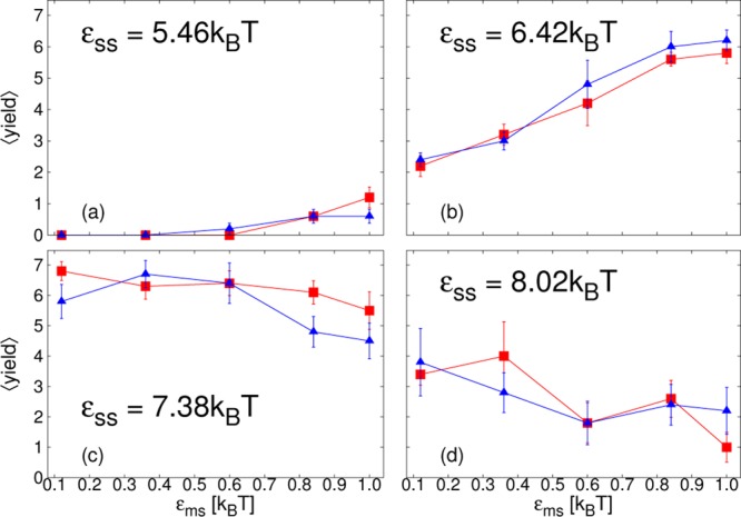
Plots of the average yield of complete cores, ⟨yield⟩, as a function of membrane-subunit interaction strength, ε_ms, for membrane stiffness, λ_b = 4√3k_BT at t = 5 × 10⁴t₀. From simulations with SRD, for different membrane viscosities: η_m = 35.1m/t₀ (blue, ▲/Δ); η_m = 1190m/t₀ (red, ■/□); and subunit interaction strengths, ε_ss, as indicated in panels a–d.

Overall, as ε_ss is increased, we identify three different trends for finite-time assembly with realistic dynamics. First, at ε_ss = 5.46k_BT and 6.42k_BT, both lower than the bulk-assembly optimal value, increasing ε_ms, which tends to increase the membrane deformation rate in all regimes, may promote finite-time assembly. With high ε_ms, assembly also occurs for values of ε_ss where there is no bulk assembly within our simulation time. However, the rate at which the membrane deforms is important. It is influenced by various factors, for example the strength of the attraction of subunits to the membrane or membrane viscosity, and results in competing effects on assembly. Increasing it via ε_ms may at first aid assembly, as seen in the initial increase in ⟨yield⟩ with ε_ms in parts a and b of Figures 5–7, but when it is too high, the yield may decrease again, as is seen particularly clearly in Figure 6a and b. Results depend on factors such as membrane viscosity and hydrodynamic interactions: decreasing membrane viscosity or including hydrodynamic interactions both increase the deformation rate. Attraction to, deformation of, and encapsulation within, the membrane is expected to decrease the subunit entropy such that the difference in entropy between unassembled and assembled states is less. Additionally, the deformation of the membrane may help to guide subunits attached to it toward each other. It is expected that these effects will all play a role in promoting assembly, although their relative importance may not be easily deduced. However, if the deformation occurs too quickly, before complete cores are formed, the membrane will hinder further subunits, or other partial cores, from approaching the partial structure, preventing its completion.

Interestingly, in this low ε_ss regime, finite-time assembly is promoted even for λ_b = 4√3k_BT, Figure 7a,b, although for this membrane stiffness budding only occurs for the highest ε_ms. For this membrane stiffness, results do not depend on membrane viscosity, confirming that here budding does not play a role. Despite a lack of envelopment, it is expected that attachment to the membrane will nonetheless reduce the entropic cost of forming a partial core. A second plausible mechanism is a local increase in subunit density near the membrane surface. In contrast, for the lower two λ_b, Figure 5a,b and Figure 6a,b, the membrane deformation rate does play a role. Comparing SRD and LD results, simulations with hydrodynamic interactions show a larger promotion of finite-time assembly as ε_ms is increased, at least initially. For some parameters the yield decreases again as ε_ms is increased further and this drop off occurs earlier with hydrodynamic interactions. Furthermore, particularly for λ_b = 2√3k_BT, membrane viscosity, η_m, is also important. Especially for SRD results, decreasing η_m shifts the point at which the finite-time yield begins to decrease to lower ε_ms. Interestingly, the effect of hydrodynamic interactions and membrane viscosity are much stronger for λ_b = 2√3k_BT than for λ_b = √3k_BT.

In the second regime, for ε_ss = 7.38k_BT, at about the bulk-assembly optimal value, increasing ε_ms tends to decrease the finite-time yield. Here, there is no strong dependence on membrane viscosity or hydrodynamic interactions and, additionally, results are quite similar for all three membrane stiffnesses. This suggests membrane deformation is not crucial, rather the decrease in yield may occur because attraction to the membrane promotes the faster assembly of partial cores, bringing the system into the monomer starvation trap that is only seen in the bulk for higher ε_ss.

Finally, for the highest ε_ss, ε_ss = 8.02k_BT, where there is a monomer starvation kinetic trap for bulk assembly, there is no clear effect of the membrane on finite-time assembly. Since assembly, at least of partial cores, occurs very quickly in the bulk, results here are likely dominated by nonmembrane-associated assembly.

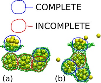
In Figure 8, we show snapshots of final configurations from simulations with λ_b = 2√3k_BT and η_m = 133.3m/t₀. For ε_ms = k_BT and ε_ss = 7.38k_BT, Figure 8a, for which the average yield was reduced compared to the low ε_ms value, three of the four cores encapsulated in a bud that are depicted are incomplete. This snapshot corresponds to the optimal ε_ss regime. In contrast, for ε_ms = 0.6k_BT and ε_ss = 6.42k_BT, Figure 8b, for which the average yield was enhanced compared to low ε_ms value, only one of the four cores encapsulated, or partially encapsulated, in a bud that are depicted is incomplete. This snapshot corresponds to the low ε_ss regime. Although these snapshots only depict the situation in two individual runs, they illustrate how the membrane may block assembly completion when its deformation rate is too high by preventing partial cores from being accessed by subunits or other partial cores.

Figure 8.

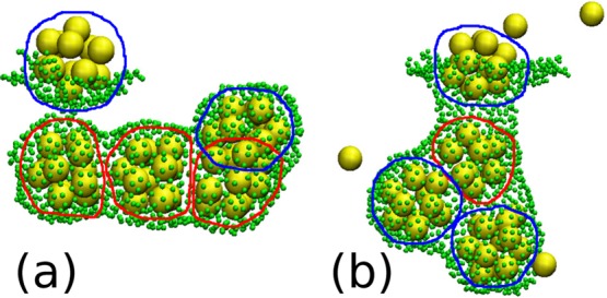
Snapshots from simulations with SRD at t = 5 × 10⁴t₀ with membrane stiffness, λ_b = 2√3k_BT and membrane viscosity, η_m = 133.3m/t₀: (a) Membrane-subunit interaction strength, ε_ms = k_BT and inter-subunit interaction strength, ε_ss = 7.38k_BT; (b) ε_ms = 0.6k_BT, ε_ss = 6.42k_BT. Subunits are shown in yellow and membrane particles in green. Only subunits within 6l₀ of a membrane particle are plotted. Membrane particle size has been reduced to make structures within buds more visible. Completed cores are circled in blue, while partially assembled ones are circled in red.

A useful quantity to indicate the amount of membrane deformation is r_frame, the distance from the edge of the simulation box of the frame to which the edge of the membrane is bound, which increases as the membrane distorts its shape out of the plane. To show how changing membrane viscosity, and including hydrodynamic interactions, alters the rate and extent of membrane deformation, we plot, in Figure 9, ⟨r_frame⟩ as a function of time with λ_b = 2√3k_BT and ε_ss = 6.42k_BT for different ε_ms from 0.36k_BT. Apart from the lowest ε_ms, the membrane deformation occurs faster and to a greater extent for simulations with hydrodynamics. Hydrodynamic interactions increase the rate of budding. Since budding requires the whole of the membrane to move, correlations mediated by hydrodynamics promote it. Furthermore, for SRD simulations at the highest two ε_ms, there are also significant differences between membrane viscosities with a trend as expected: ⟨r_frame⟩ is largest for the smallest viscosity.

Figure 9.

Plots of the average position of the frame, ⟨r_frame⟩, as a function of time, t, for membrane stiffness, λ_b = 2√3k_BT and inter-subunit interaction strength, ε_ss = 6.42k_BT. From simulations with SRD (solid lines, filled symbols) or LD (dashed lines, open symbols), for different membrane viscosities: η_m = 35.1m/t₀ (blue, ▲/Δ); η_m = 133.3m/t₀ (green, ●/○); η_m = 1190m/t₀ (red, ■/□); and subunit-membrane interaction strengths: (a) ε_ms = 0.36k_BT; (b) ε_ms = 0.6k_BT; (c) ε_ms = 0.84k_BT; (d) ε_ms = k_BT.

We next consider the distributions of cluster size, n_c, in our SRD simulations, H(n_c). In Figure 10, we plot distributions for λ_b = 2√3k_BT and η_m = 35.1m/t₀ at three different times. For ε_ss = 6.42k_BT, the lowest ε_ss for which, in dynamical simulations, there is bulk assembly, there are few clusters with intermediate sizes when ε_ms is low. At all times considered, the majority of clusters are of size two; at later times there is an additional peak at size 12, corresponding to complete cores. In contrast, when ε_ms is high, the attraction to the membrane stabilizes intermediate cluster sizes at early times. At later times, the clusters have grown but the peak near 12 is less sharp, with similar numbers of cores of size 10 and 11, and also some larger ones. This shows the effect of the membrane blocking the completion of partial cores. It also seen for higher ε_ss, ε_ss = 7.38k_BT, where the distribution for low ε_ms is much flatter at early times with many clusters of intermediate sizes.

Figure 10.

Results from SRD simulations. Histograms, H, of cluster size, n_c, for membrane stiffness, λ_b = 2√3k_BT and membrane viscosity, η_m = 35.1m/t₀ at different times, t: t = 1 × 10⁴t₀ (red); t = 3 × 10⁴t₀ (green); t = 5 × 10⁴t₀ (blue); with different parameters: (a) Membrane-subunit interaction strength, ε_ms = 0.12k_BT and inter-subunit interaction strength, ε_ss = 6.42k_BT; (b) ε_ms = k_BT, ε_ss = 6.42k_BT; (c) ε_ms = 0.12k_BT, ε_ss = 7.38k_BT; (d) ε_ms = k_BT, ε_ss = 7.38k_BT.

In Figure 11, we show the effect of membrane viscosity on the cluster size distribution. We plot results from the end of the simulations, at time t = 5 × 10⁴t₀, again for λ_b = 2√3k_BT. With ε_ss = 6.42k_BT, we see that, for the highest viscosity, increasing ε_ms leads to a distribution that is more strongly peaked at 12. In contrast, for the lowest viscosity, although increasing ε_ms does lead to more larger clusters, it also gives a much broader distribution around 12. A similar effect occurs for ε_ss = 5.46k_BT: for this ε_ss too, when membrane viscosity is low, high ε_ms causes the membrane to encapsulate the assembling capsids too quickly, blocking their completion.

Figure 11.

Results from SRD simulations. Histograms, H, of cluster size, n_c, for membrane stiffness, λ_b = 2√3k_BT at time, t = 5 × 10⁴t₀ for different membrane-subunit interaction strength values: ε_ms = 0.12k_BT (red); ε_ms = 0.6k_BT (green); ε_ms = k_BT (blue); with different parameters: (a) Membrane viscosity, η_m = 1190m/t₀ and inter-subunit interaction strength, ε_ss = 6.42k_BT; (b) η_m = 35.1m/t₀, ε_ss = 6.42k_BT; (c) η_m = 1190m/t₀, ε_ss = 5.46k_BT; (d) η_m = 35.1m/t₀, ε_ss = 5.46k_BT.

As in similar previous models,⁵ the concentration of our subunits is relatively high compared to experimental systems, and furthermore the number of subunits in a completed core is low. These choices are necessary for computational tractability but have the consequence that the assembly rates in our simulations are much higher than experimental ones. Assuming that subunits correspond to capsomers of size on the order of 10 nm, and matching the drag coefficient of our subunits, we estimate that our simulation length is around 5 ms, whereas in vitro(24) and in vivo(52) experiments have observation times on the order of minutes. Thus, a direct quantitative comparison cannot be made. Our results rather demonstrate how the rate of membrane deformation compared to the assembly rate may affect the success of the latter. Furthermore, they show how properties such as membrane viscosity, which might be varied experimentally by changing lipid composition⁵³ are expected to impact on the assembly process. The interactions between assembling viral capsomers are typically relatively weak⁵⁴ as this aids the avoidance of kinetic traps and thus the first, low ε_ss regime identified is most likely to be relevant to these systems.

6. Other Target Cores

We have investigated the effect of a membrane on core assembly of icosahedral cores. It is expected that many of the qualitative features of the results, such as the interplay between the membrane promoting assembly by confining subunits and hindering it by blocking additional subunits or other partial cores from approaching partial structures, will be general to other target structures. To gain more insight into the transferability of the findings to other core shapes, we finally, in Figure 12, present results on the yield obtained in SRD simulations when the target structure is changed from the icosahedral core. As for icosahedra, we define a cluster to be a complete structure when it contains the correct number of subunits for the target structure and each subunit patch on each subunit forms a bond with another member of the cluster. We choose subunits with patches such that their interactions are minimized for cubic and dodecahedral structures.⁶ Otherwise, parameters such as patch width are unchanged, with the membrane patch still lying on the symmetry axis as defined by the subunit patches and pointing outward in a complete structure. In both cases, the subunits only have three patches for bonding with other subunits and thus form fewer bonds in a complete structure than the icosahedral subunits. Correspondingly, the range of ε_ss was shifted up by about 2k_BT but the range of ε_ms remained the same.

Figure 12.

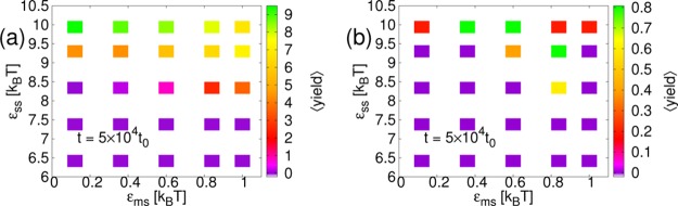
Results from SRD simulations. Plots of the average yield of complete structures, ⟨yield⟩, as a function of membrane-subunit interaction strength, ε_ms and inter-subunit interaction strength, ε_ss at time t = 5 × 10⁴t₀ for membrane stiffness, λ_b = 2√3k_BT and membrane viscosity, η_m = 133.3m/t₀: (a) Subunits with interactions to form a cube. (b) Subunits with interactions to form a dodecahedron. Note the different scales for ⟨yield⟩ and also the higher values of ε_ss as compared to the results for icosahedral cores.

We simulated for λ_b = 2√3k_BT and η_m = 133.3m/t₀. For both cubes and dodecahedra, as for icosahedra, budding of the membrane occurred for high ε_ms. In Figure 12a, many of the features of the finite-time assembly of icosahedra are reproduced for cubes. For high ε_ms, there is finite-time assembly at lower ε_ss than for low ε_ms. There is also an increase in finite-time yield with increasing ε_ms for the lowest ε_ss for which assembly occurs without significant attraction to the membrane. Unlike for icosahedra, at least for these membrane parameters, the yield does not drop off again as ε_ms is increased further. This may be because, since they are composed of less subunits, cubes assemble faster than icosahedra. For the highest ε_ss, however, there is a reduction in finite-time yield with ε_ms, similar to results for icosahedra.

As observed in previous work,⁶ finite-time yields of dodecahedra, Figure 12b, were low. However, here again, there is evidence that attraction to the membrane may promote assembly for ε_ss for which it would otherwise not occur. Although it is not apparent in our results, as seen in previous work with a very similar model,⁶ it is expected that, if the subunit interaction strength were increased sufficiently, the same nonmembrane-related kinetic trap that is observed for icosahedra would also be seen for cubes and dodecahedra.

7. Conclusions

To summarize, we have applied a simple patchy-particle model to investigate the effect of interactions with a fluctuating membrane on the dynamics of the assembly of core structures with the same symmetry as many viral cores. As well as interaction strengths, the key parameters we varied were membrane stiffness and viscosity. We also considered the effect of hydrodynamic interactions by simulating both with SRD and LD. As at equilibrium, for assembly with realistic dynamics, attraction to a membrane may promote finite-time assembly, also for subunit interaction strengths, ε_ss, for which it does not occur in the bulk. Furthermore, for ε_ss less than the optimal bulk value, attraction to the membrane also decreases the single-core assembly time.

Membrane budding occurred in dynamically realistic simulations and its rate was strongly increased by hydrodynamic interactions, as well as by lowering the membrane viscosity. The rate of membrane deformation is important in determining the assembly yield after finite time. Relatively high rates may promote assembly by increasing the envelopment of assembling cores and thus decreasing the entropic penalty and also by guiding subunits toward each other. However, if the rate is too high, the membrane may block partial cores from being completed. Three regimes with different effects of the membrane were identified. For ε_ss less than the bulk optimum, finite-time yields depend intricately on a combination of all parameters and may both increase and decrease as attraction to the membrane is increased. For ε_ss about equal to the bulk optimum, finite-time yields do not depend strongly on the membrane deformation rate and tend to decrease as attraction to the membrane is increased. For ε_ss higher than the bulk optimum, assembly in the bulk is affected by a monomer starvation kinetic trap and the membrane has little influence.

Finally, results with qualitative similarities were also found for core structures with cubic and dodecahedral symmetries. In future work it would be interesting to investigate more different structures, in particular much larger cores.

Supporting Information Available

Definitions of the functions used in interparticle interactions and the confinement of membrane particles to the frame. This material is available free of charge via the Internet at http://pubs.acs.org.

The authors declare no competing financial interest.

References

- Hagan M. F. Adv. Chem. Phys. 2013, arXiv:1301.1657. [Google Scholar]
- Fraenkel-Conrat H.; Williams R. Proc. Natl. Acad. Sci. U.S.A. 1955, 41, 690–698. [DOI] [PMC free article] [PubMed] [Google Scholar]
- Rapaport D. Phys. Rev. E 2004, 70, 051905. [DOI] [PubMed] [Google Scholar]
- Nguyen H.; Brooks C. III Nano Lett. 2008, 8, 4574–4581. [DOI] [PMC free article] [PubMed] [Google Scholar]
- Hagan M.; Chandler D. Biophys. J. 2006, 91, 42–54. [DOI] [PMC free article] [PubMed] [Google Scholar]
- Wilber A.; Doye J.; Louis A.; Lewis A. J. Chem. Phys. 2009, 131, 175102. [DOI] [PubMed] [Google Scholar]
- Johnston I.; Louis A.; Doye J. J. Phys.: Condens. Matter 2010, 22, 104101. [DOI] [PubMed] [Google Scholar]
- Elrad O. M.; Hagan M. F. Phys. Biol. 2010, 7, 045003. [DOI] [PMC free article] [PubMed] [Google Scholar]
- Mahalik J.; Muthukumar M. J. Chem. Phys. 2012, 136, 135101. [DOI] [PMC free article] [PubMed] [Google Scholar]
- Sun J.; DuFort C.; Daniel M.-C.; Murali A.; Chen C.; Gopinath K.; Stein B.; De M.; Rotello V. M.; Holzenburg A.; Kao C. C.; Dragnea B. Proc. Natl. Acad. Sci. U.S.A. 2007, 104, 1354–1359. [DOI] [PMC free article] [PubMed] [Google Scholar]
- Elrad O. M.; Hagan M. F. Nano Lett. 2008, 8, 3850–3857. [DOI] [PMC free article] [PubMed] [Google Scholar]
- Williamson A. J.; Wilber A. W.; Doye J. P.; Louis A. A. Soft Matter 2011, 7, 3423–3431. [Google Scholar]
- Gelderblom H.; Hausmann E.; Özel M.; Pauli G.; Koch M. Virology 1987, 156, 171–176. [DOI] [PubMed] [Google Scholar]
- Ono A. Vaccine 2010, 28, B55–B59. [DOI] [PMC free article] [PubMed] [Google Scholar]
- Miyanari Y.; Atsuzawa K.; Usuda N.; Watashi K.; Hishiki T.; Zayas M.; Bartenschlager R.; Wakita T.; Hijikata M.; Shimotohno K. Nat. Cell Biol. 2007, 9, 1089–1097. [DOI] [PubMed] [Google Scholar]
- Shavinskaya A.; Boulant S.; Penin F.; McLauchlan J.; Bartenschlager R. J. Biol. Chem. 2007, 282, 37158–37169. [DOI] [PubMed] [Google Scholar]
- Forsell K.; Xing L.; Kozlovska T.; Cheng R.; Garoff H. EMBO J. 2000, 19, 5081–5091. [DOI] [PMC free article] [PubMed] [Google Scholar]
- Ng C.; Coppens I.; Govindarajan D.; Pisciotta J.; Shulaev V.; Griffin D. Proc. Natl. Acad. Sci. U.S.A. 2008, 105, 16326–16331. [DOI] [PMC free article] [PubMed] [Google Scholar]
- Simon L. Proc. Natl. Acad. Sci. U.S.A. 1972, 69, 907–911. [DOI] [PMC free article] [PubMed] [Google Scholar]
- Siegel P.; Schaechter M. Annu. Rev. Microbiol. 1973, 27, 261–282. [DOI] [PubMed] [Google Scholar]
- Bravo A.; Salas M. J. Mol. Biol. 1997, 269, 102–112. [DOI] [PubMed] [Google Scholar]
- Matthews R.; Likos C. N. Phys. Rev. Lett. 2012, 109, 178302. [DOI] [PubMed] [Google Scholar]
- Frenkel D.; Smit B.. Understanding Molecular Simulation: from Algorithms to Applications; Academic Press: London, 2002. [Google Scholar]
- Zlotnick A.; Aldrich R.; Johnson J. M.; Ceres P.; Young M. J. Virology 2000, 277, 450–456. [DOI] [PubMed] [Google Scholar]
- Kikuchi N.; Gent A.; Yeomans J. Eur. Phys. J. E 2002, 9, 63–66. [DOI] [PubMed] [Google Scholar]
- Whitmer J. K.; Luijten E. J. Phys. Chem. B 2011, 115, 7294–7300. [DOI] [PubMed] [Google Scholar]
- Šarić A.; Cacciuto A. Phys. Rev. Lett. 2012, 108, 118101. [DOI] [PubMed] [Google Scholar]
- Reynwar B.; Illya G.; Harmandaris V.; Müller M.; Kremer K.; Deserno M. Nature 2007, 447, 461–464. [DOI] [PubMed] [Google Scholar]
- Zhang R.; Nguyen T. T. Phys. Rev. E 2008, 78, 051903. [DOI] [PubMed] [Google Scholar]
- Šarić A.; Cacciuto A. Phys. Rev. Lett. 2012, 109, 188101. [DOI] [PubMed] [Google Scholar]
- Bahrami A. H.; Lipowsky R.; Weikl T. R. Phys. Rev. Lett. 2012, 109, 188102. [DOI] [PubMed] [Google Scholar]
- Bianchi E.; Blaak R.; Likos C. N. Phys. Chem. Chem. Phys. 2011, 13, 6397–6410. [DOI] [PubMed] [Google Scholar]
- Gompper G.; Kroll D. J. Phys. I 1996, 6, 1305–1320. [Google Scholar]
- Noguchi H.; Gompper G. Phys. Rev. E 2005, 72, 11901. [DOI] [PubMed] [Google Scholar]
- Matthews R.; Likos C. N. Soft Matter 2013, 9, 5794–5806. [Google Scholar]
- Ouldridge T. E.; Louis A. A.; Doye J. P. J. Phys.: Condens. Matter 2010, 22, 104102. [DOI] [PubMed] [Google Scholar]
- Lerner D. M.; Deutsch J. M.; Oster G. F. Biophys. J. 1993, 65, 73–79. [DOI] [PMC free article] [PubMed] [Google Scholar]
- Gompper G.; Ihle T.; Kroll D.; Winkler R. Adv. Polym. Sci. 2009, 221, 1–87. [Google Scholar]
- Dünweg B. Langevin Methods. In Computer Simulations of Surfaces and Interfaces; Proceedings of the NATO Advanced Study Institute; Kluwer Academic: Norwell, MA, 2003; pp 77–92. [Google Scholar]
- Ladd A. J. Comput. Phys. Commun. 2009, 180, 2140–2142. [Google Scholar]
- Faller R.; Yan Q.; De Pablo J. J. Chem. Phys. 2002, 116, 5419. [Google Scholar]
- Mehlig B.; Heermann D.; Forrest B. Phys. Rev. B 1992, 45, 679–685. [DOI] [PubMed] [Google Scholar]
- Chen B.; Siepmann J. J. Phys. Chem. B 2001, 105, 11275–11282. [Google Scholar]
- Kikuchi N.; Pooley C.; Ryder J.; Yeomans J. J. Chem. Phys. 2003, 119, 6388. [Google Scholar]
- Whitmer J.; Luijten E. J. Phys.: Condens. Matter 2010, 22, 104106. [DOI] [PubMed] [Google Scholar]
- Padding J.; Wysocki A.; Löwen H.; Louis A. J. Phys.: Condens. Matter 2005, 17, S3393. [Google Scholar]
- Padding J.; Louis A. Phys. Rev. E 2006, 74, 031402. [DOI] [PubMed] [Google Scholar]
- Pettit F. K.; Bowie J. U. J. Mol. Biol. 1999, 285, 1377–1382. [DOI] [PubMed] [Google Scholar]
- Belushkin M.; Winkler R.; Foffi G. Soft Matter 2012, 8, 9886–9891. [Google Scholar]
- Petrov E. P.; Schwille P. Biophys. J. 2008, 94, L41–L43. [DOI] [PMC free article] [PubMed] [Google Scholar]
- Baker T.; Olson N.; Fuller S. Microbiol. Mol. Biol. Rev. 1999, 63, 862–922. [DOI] [PMC free article] [PubMed] [Google Scholar]
- Baumgärtel V.; Müller B.; Lamb D. C. Viruses 2012, 4, 777–799. [DOI] [PMC free article] [PubMed] [Google Scholar]
- Espinosa G.; López-Montero I.; Monroy F.; Langevin D. Proc. Natl. Acad. Sci. U.S.A. 2011, 108, 6008–6013. [DOI] [PMC free article] [PubMed] [Google Scholar]
- Zlotnick A. Virology 2003, 315, 269–274. [DOI] [PubMed] [Google Scholar]
- Humphrey W.; Dalke A.; Schulten K. J. Mol. Graphics 1996, 14, 33–38. [DOI] [PubMed] [Google Scholar]
Associated Data
This section collects any data citations, data availability statements, or supplementary materials included in this article.