Network-guided sparse regression modeling for detection of gene-by-gene interactions

Abstract

Motivation: Genetic variants identified by genome-wide association studies to date explain only a small fraction of total heritability. Gene-by-gene interaction is one important potential source of unexplained total heritability. We propose a novel approach to detect such interactions that uses penalized regression and sparse estimation principles, and incorporates outside biological knowledge through a network-based penalty.

Results: We tested our new method on simulated and real data. Simulation showed that with reasonable outside biological knowledge, our method performs noticeably better than stage-wise strategies (i.e. selecting main effects first, and interactions second, from those main effects selected) in finding true interactions, especially when the marginal strength of main effects is weak. We applied our method to Framingham Heart Study data on total plasma immunoglobulin E (IgE) concentrations and found a number of interactions among different classes of human leukocyte antigen genes that may interact to influence the risk of developing IgE dysregulation and allergy.

Availability: The proposed method is implemented in R and available at http://math.bu.edu/people/kolaczyk/software.html.

Contact: chenlu@bu.edu

Supplementary information: Supplementary data are available at Bioinformatics online.

1 INTRODUCTION

Unlike Mendelian diseases, in which disease phenotypes are largely driven by mutation in a single gene locus, complex disease and traits are associated with a number of factors, both genetic and environmental, as well as lifestyle. In addition, while most Mendelian diseases are rare, many complex diseases are frightfully common, from asthma to heart disease, hypertension to Alzheimer’s and Parkinson’s to various forms of cancer.

Arguably motivated by classical successes with Mendelian diseases and traits, the study of complex diseases and traits in the modern genomics era has focused largely on the identification of individually important genes. Genome-wide association studies (GWAS), the current state of the art, have been central to the discovery of many genes in various diseases (e.g. Hindorff et al., 2010). However, unfortunately, the vast majority of genetic variants associated with complex traits identified to date explain only a small amount of the overall variance of the trait in the underlying population (Manolio et al., 2009). As a result, most GWAS findings thus far have had little clinical impact.

Currently, most GWAS are carried out one single nucleotide polymorphism (SNP) at a time. Typically, for each SNP, a model is specified, relating disease status or disease trait to the SNP plus other potentially relevant covariates. The statistical significance of each SNP is quantified through the P-value of an appropriate test. Finally, a multiple-testing correction is applied to correct the collection of P-values across SNPs. The end result is a list of SNPs declared to be significantly associated with the status or trait of interest, which in turn can be mapped to their closest genes, although some associations have been found in ‘gene deserts’ (Hindorff et al., 2010). The single-SNP approach has the important attribute that it is (relatively) computationally efficient. However, it can be severely under-powered because of the small effect size of most genetic variants identified to date (Hindorff et al., 2010; Manolio et al., 2009). Additionally, this approach does not adjust for correlation among SNPs, nor does it extend in a natural manner to search for interactions between markers. In contrast, multiple regression (i.e. where multiple SNPs are modeled simultaneously) is a natural alternative. However, naive implementation (i.e. incorporating all SNPs of interest) is both infeasible and undesirable. This is due to various reasons, including the sheer number of SNPs typically available (e.g. hundreds of thousands to millions), the comparatively small number of SNPs likely to be associated and ‘small n, large p’ problems.

Recently, however, computationally efficient multiple regression strategies for GWAS have begun to emerge that use various methods of high-dimensional variable selection (e.g. Ayers and Cordell, 2010; Logsdon et al., 2010; Ma et al., 2010; Szymczak et al., 2009; Wu et al., 2009, 2010; Zhou et al. 2010). Compared with traditional single-SNP methods, penalized regression methods have been found to yield fewer correlated SNPs (Ayers and Cordell, 2010) and to be capable of producing substantially more power while having a lower false-discovery rate (FDR; He and Lin, 2011). Furthermore, and most relevant to the current article, regression methods can include SNP by SNP interactions in a natural manner. However, to date, this typically has been done in a greedy stage-wise manner, by fitting main-effect models first and then restricting attention to interactions among those effects found significant (Wu et al., 2009, 2010). In addition, the above work makes limited or no use of supplementary biological information on, for example, biological pathways and gene function.

We propose a novel network-guided statistical methodology to facilitate the discovery of gene-by-gene (G × G) interactions associated with complex quantitative traits related to human disease, one which addresses both of the shortcomings cited above. Main effects and interaction effects in our model are chosen simultaneously, thus allowing for the possibility of detecting genes for which the marginal main effect is weak. Variable selection is done through penalized regression using sparse estimation principles. The penalty allows for the incorporation of information on biological pathways and gene function into the analysis of continuous traits related to human disease. In doing so, this penalty acts as an informal prior distribution on the set of possible G × G interactions, which in practice allows the investigator to reduce the number of interactions examined for the model from the nominal and computationally prohibitive O((number of SNPs)²) to a more manageable, say, O(number of SNPs).

Simulations indicate that, given relevant pathway information, our approach performs well in finding true interactions without losing the ability of detecting main effects, and can noticeably outperform existing stage-wise methods. In addition, application of our proposed methodology to a study of plasma total immunoglobulin E (IgE) concentrations for participants in the Framingham Heart Study (FHS) illustrates the substantial promise of the method.

The rest of this article is organized as follows: in Section 2, we describe our statistical approach. We introduce the model and our proposed penalty, describe how biological information is incorporated into the penalty and explain the optimization algorithm used for model fitting and a strategy for choosing tuning parameters. The design and results of an extensive simulation study are presented in Section 3, in which we examine models with varying degrees of interactions and penalties reflecting different extents of biological knowledge. Our analysis of the IgE concentration data is provided in Section 4. Some additional discussion may be found in Section 5.

2 METHODS

2.1 Modeling G × G interaction

Let Y be a quantitative trait of interest, and let be p predictors representing SNPs. To include interactions, we are interested in a model of the form

(1)

where . We expect that both the s and the s are sparse, as it is unlikely that there is more than a small fraction of SNPs affecting the phenotype Y, either as main effects or as interactors.

In practice, p will range from hundreds to millions. Our goal is to fit the high-dimensional model (1) to data. When p is large but only a small percentage of predictors and interactions are present in the true model, a general approach is to minimize a penalized regression criterion. Accordingly, we propose to estimate the coefficients in our model using a penalized least-squares criterion. Let and represent our variables and collected over n samples. Our criterion is then written as follows:

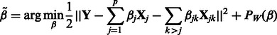(2)

Penalized linear regression has been found to be a powerful tool for fitting high-dimensional models, particularly in situations where the nominal number of variables is large relative to the number of observations (e.g. Bühlmann and Van De Geer, 2011). In the context of GWAS, typically . Hence, it is impossible to fit a model with the full set of nominal interactions among all p SNPs. However, the coefficient vector is expected to be sparse. Therefore, a penalty function that enforces sparseness can be helpful here, by encouraging the optimization in (2) to find solutions in which a large percentage of the main effects and their interactions are zero, thus dropping the corresponding terms from the model.

Following standard practice, we wish to include interactions only if their corresponding main effects are also included in the model. The construction of the sparseness penalty , therefore, must be handled with some care, so as to enforce the resulting hierarchical constraint among coefficients. In addition, we would like our penalty to allow for the use of biological knowledge (e.g. biological pathways, gene functional classes, etc.) in fitting the model. We address these two goals by defining a penalty of the form

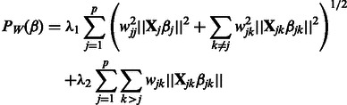(3)

where the are non-negative weights provided by the investigator, and is used to denote the matrix of weights over all SNP pairs . The values are tuning parameters.

Our penalty is a generalization of that proposed by Radchenko and James (2010) for the purpose of fitting general types of interaction models (in Radchenko and James (2010), for all ). Note that, following those authors, we express the penalty in un-normalized form (standard lasso algorithms, for example, without interactions, assume and hence ). It can be shown that the penalty automatically enforces the hierarchical constraint (i.e. inclusion of main effects before interactions). Main effects and interactions can be treated differently by varying with respect to . The elements of the matrix W are generic and allow for the possibility of including biological information a priori into the model selection process. We next describe a manner for doing so, in which network principles are used in a natural way.

2.2 A network-based penalty

Here we describe how we construct the matrix W, using information on biological pathways. Similar constructions may be had generally using other common resources (e.g., databases of genes and their biological function, such as Gene Ontology). Note that W acts as a dissimilarity matrix in . Under our construction, W is defined in association with a graph showing relationships among SNPs, which in turn derives from a bipartite graph relating SNPs to pathways. The intuition underlying our construction is to (i) allow interactions only among SNPs corresponding to genes that are common to at least one pathway, and (ii) to encourage interactions more among those SNP pairs that are common to more pathways.

Let denote our p SNPs, and , our m pathways. We define G to be a bipartite graph, with one set of nodes representing SNPs, and the other, pathways. An edge in G connects an SNP to a pathway if that SNP maps sufficiently close to a gene found in the pathway. We then define to be the one-mode projection of G onto the set of SNPs. Figures 1 and 2 show three toy examples of graphs G and , for SNPs and pathways.

Fig. 1.

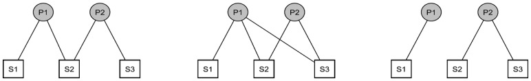
Simple illustration of network representations between SNPs (S1, S2, S3) and pathways (P1, P2)

Fig. 2.

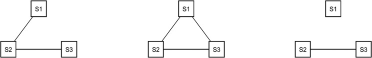
One-mode projection of the three examples in Figure 1

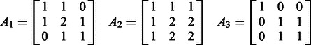
An equivalent representation of the relationship between SNPs and pathways in the network is a incidence matrix M, describing which SNPs are linked to which pathways. For the three examples in Figure 1, the corresponding incidence matrices are

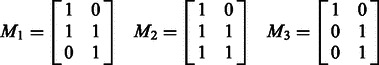(4)

Similarly, the analogous (weighted) adjacency matrix is the standard representation of the one-mode projection . Calling this matrix A, it is related to the incidence matrix M of the original graph G through the expression . For the three examples shown in Figure 1 and Figure 2, the adjacency matrices are

(5)

Finally, we define the dissimilarity matrix W element-wise by setting . In the case where , we set by convention. Note that the resulting implication for the optimization in (2) is that is set to zero, i.e. the term cannot enter the model. Hence, only those pairs of SNPs that share at least one pathway (i.e. ) may potentially enter the model. As a result, it is possible to substantially reduce the number of interaction terms considered for entry into the model, thus making the simultaneous search for main effects and interactions easier to perform. For example, in the application presented in Section 4, 17 025 SNPs were used, nominally corresponding to ∼145 million interactions. However, in using the 186 pathways from the Kyoto Encyclopeida of Genes and Genomes (KEGG) database to construct our matrix W, this number was reduced to less than 480 000 potential interactions.

We note that there are certainly other ways of constructing the matrix W. For example, a variation on the procedure described above would be to define if , and infinity otherwise. This is equivalent to equipping the graph with a binary adjacency matrix and letting as before, and results in the equal treatment of all interactions that are allowed to enter the model, regardless of how many pathways are shared by pairs . In addition, of course, other types of outside information—if judged relevant—can be used in place of pathways, as mentioned above.

2.3 Model selection and fitting

To perform the optimization in (2), we use cyclic coordinate descent, a now-standard choice for problems such as ours (e.g. Friedman et al., 2007; Wu and Lange, 2008; Wu et al., 2009). As the name indicates, the cyclic coordinate descent algorithm updates one element of at a time using coordinate descent principles, while holding all others fixed, and cycles through all elements until convergence. In our context, the details of the resulting algorithm parallel those of Radchenko and James (2010). We, therefore, present only a sketch of the algorithm and relevant formulas here. Detailed derivation can be found in Supplementary Material, Section 1.

Consider the estimation of . We note that, with respect to this parameter, the objective function in (2) can be written as

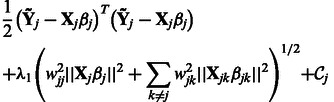(6)

where . Here is the current value of at this stage of our iterative algorithm, and similarly for , while is all of the rest of the penalty term that does not involve .

The updates to the estimates of the main effects take the form of a shrinkage estimate, , for . Here is the solution to the problem of fitting a regression-through-the-origin for on , and the shrinkage parameter is the solution to the equation

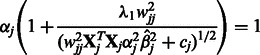(7)

where 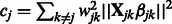. The value can be obtained using the Newton–Raphson method. In the special case where , which must be the case when for all (i.e. SNP j is not allowed to participate in any interactions), Equation (7) can be solved in closed form, yielding .

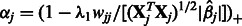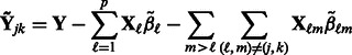
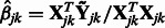Now consider the estimation of . Similar arguments show that the iterations in the cyclic coordinate descent algorithm involve updates of the form , for . Here is the solution to the problem of fitting a regression-through-the-origin for on , where

The shrinkage parameter for interaction terms is the solution to the equation

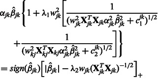(8)

where

and

which again can be computed using the Newton–Raphson method. When and are both zero, can be solved in closed form, yielding

The shrunken estimates of coefficients of predictors and interactions are updated in the iterative process described above until convergence is achieved. Following standard practice, on termination of our cyclic coordinate descent algorithm, we generate a final estimate of coefficients for those variables and that were allowed to enter the model, using ordinary least squares. All corresponding effect-size estimates and P-values produced by our methodology result from this final step.

For datasets with a small number of predictors , the algorithm can be easily fit as described. However, for larger numbers of predictors, we use a ‘swindle’, in analogy to that proposed by Wu et al. (2009) and implemented in MENDEL (Lange et al., 2001). The basic idea is to apply the algorithm to a much smaller number, say k, of pre-screened predictors, and to choose the smoothing parameter(s) such that only a desired number, say , of predictors enters the model. The Karush–Kuhn–Tucker (KKT) conditions for our optimization problem are then checked for the estimate resulting from our algorithm (augmented with zeros for coefficients of all predictors eliminated at the pre-screening stage). If the KKT conditions are satisfied, we are done; if not, we double k and repeat the process. Following Wu et al. (2009), we let our initial choice of k be a multiple of s, i.e. in the applications we show. Pre-screening consists of sorting the t statistics of fitting ordinary least-square regression of Y on each predictor separately (i.e. traditional GWAS) and extracting those predictors with the k largest t statistics. Details can be found in Supplementary Material, Section 2.

2.4 Choice of tuning parameters

In the penalty function defined in (3), the tuning parameters directly influence the number of variables that enter the final model. In principle, these two parameters may be allowed to vary freely and a cross-validation strategy used to select the best values. However, this strategy is unrealistic for GWAS, where the number of SNPs may range into millions. Instead, we use a strategy that allows investigators some control in dictating how many variables enter the model, and thereby specify the tuning parameters implicitly.

First, we impose a linear relation between the two tuning parameters, i.e. . Because is directly involved only in the selection of interaction terms, specifying the constant c may be interpreted as ‘tuning’ the number of interactions relative to main effects. The tuning parameter is responsible for the number of main effects in the model. Because is essentially a decreasing function of the number of main effects entered in the model and often investigators have at least some rough expectation of how many SNPs they feel are likely to be associated with their phenotype, we set by pre-specifying the number of main effects to include in the final model (i.e. denoted s above).

Second, calculations show that the relation holds, where is the variance of SNP j coded as the number of minor alleles under the assumption of Hardy–Weinberg equilibrium; the variance is defined here in terms of the minor allele frequency (MAF) , and r is the ratio of the thresholds for main effects and interactions to enter the model within the cyclic coordinate descent algorithm. See Supplementary Material, Section 3, for details. We recommend that c be chosen by the user through (i) specifying a desired ratio r and (ii) knowledge of the distribution of SNP MAFs.

By setting the desired number of main effects and the value c, we implicitly specify the values of the tuning parameters . A smaller value of c (corresponding to a larger value of r) means more interactions may enter the model, for a fixed number of main effects.

3 SIMULATION

3.1 Simulation study design

We carried out a simulation study to assess (i) the performance of our method under various interaction scenarios and (ii) the effect of different choices of the W matrix in our penalty on our ability to detect interaction. We also compared our method with the stage-wise selection method proposed by Wu et al. (2009), which restricts interaction search to SNPs first declared to have main effects. In each simulated dataset, there are 1000 subjects and 1000 SNPs as predictors. The SNPs are coded additively (0, 1, 2), simulated with a MAF of 50%, and drawn from a binomial distribution with two trials. Lower MAFs were also investigated (MAF ≥ 10%, see Supplementary Material, Section 4.5). The quantitative trait Y is then simulated using the effect SNPs and interactions specified under assumed models. The effect sizes are set for 80% power under standard single-SNP additive models. Among the 1000 SNPs, 20 (SNPs 1–20) have true main effects on the simulated trait, and the remaining 980 SNPs have no effect.

To test our method in various interaction situations, we evaluate three different models:

• Model 1: only 20 main effects with no interaction,

• Model 2: 20 main effects + all two way interactions among SNPs 1–5, and

• Model 3: 20 main effects + SNP1 × SNP2 + SNP3 × SNP4 + SNP5 × SNP6 + … + SNP19 × SNP20.

Model 1 has no interactions involved. Models 2 and 3 both have 10 interaction terms involved, and the interactions are all among true main effects. However, in Model 2, there is one cluster with 5 interacting SNPs, while in Model 3 there are 10 clusters, each with two interacting SNPs.

In addition, we explore six different ways to construct the W matrix used in the penalty. In each case, we allow all SNPs to be evaluated as possible main effects, by having all ones down the diagonal of W. For the possible interaction terms, coded by the off-diagonal elements of W, we consider the following additions:

• : + true interactions in models,

• : + two-way interactions among all true main effects (SNPs 1–20),

• : + true interactions + random ‘noise’ interactions,

• : + two-way interactions among all true main effects + random ‘noise’ interactions,

• : + two-way interactions among SNPs 1–40 (all true main effects and 20 non-active SNPs), and

• : + two-way interactions among SNPs 1–10 and 21–30 + two-way interactions among SNPs 11–20 and 31–40.

The matrix is an ideal case. It only allows true interactions built in the model to enter that model. Note that is different for each of Models 1, 2 and 3. The matrix introduces some ‘noise’ interactions by allowing all interactions among true main effects. It is equivalent to a single pathway of SNPs 1–20 and is the same for all models. The matrix adds random ‘noise’ interactions to , while adds random ‘noise’ interactions to . Note that and both vary across models. The random ‘noise’ interactions are introduced in a manner aimed at mimicking the interaction structure corresponding to the KEGG database, only some subset of which will likely be relevant to any given study (and the rest, ‘noise’). Specifically, an additional set of ‘pathways’ (i.e. gene sets) were defined, in addition to those defined by the models themselves, until 20 pathways were formed. To these 20, we then randomly allocated 160 additional SNPs so that the average number of SNPs per pathway roughly mimicked what is observed in KEGG. represents a single pathway of SNPs 1–40, similar to but with more SNPs (20 non-active SNPs) involved. then represents two pathways with each having 10 active and 10 non-active SNPs. It is similar to in the sense that the allowed interactions involve SNPs 1–40, but has smaller amount of non-active interactions.

We chose by setting the desired number of main effects selected as 25, the value of is automatically determined by our program once the value 25 is provided. This is a natural choice because there are 1000 SNPs in our data and 20 true main effects in the models. This choice will affect type I error because at least 5 of the 25 predictors selected as main effects will be false, but this number is modest compared with the total of 1000 SNPs and can be easily adjusted by resetting according to investigator preference. The parameter c is set to 0.5 (i.e. under our model). The selected predictors are then ranked by their absolute t-values resulting from the ordinary least-square fit on the selected predictors for the final model. By setting a threshold on the rank, we choose the number of interactions to be reported and compare the performance of interaction selection under various W matrix specifications across a range of thresholds.

3.2 Simulation results

In Figure 3, we compare the results under various W matrix specifications, for Models 2 and 3. We assess the ability to find true interactions by computing the average FDR of interactions over 100 trials and plotting 1 − FDR against the rank threshold for selected interactions. As the threshold increases, more interactions get selected, and thus FDR increases and the curves have a downward trend. Examining the results, we see that clearly has the best performance, as it reflects the truth about the interactions in the model; all false interactions are excluded a priori, and thus the 1 − FDR curve for is a straight line at 1. Recall that is equivalent to plus random ‘noise’. Importantly, therefore, we note that pure ‘noise’ among non-active SNPs does not appear to impact much the selection of true interactions, as has the second best performance after . This conclusion is reinforced by the results for and , where the 1 − FDR curves are nearly identical. In contrast, the results in Figure 3 also suggest that selection of interactions is to some extent adversely affected when allowing ‘noise’ interactions among active SNPs, as has better performance than and , while and have similar performance.

Fig. 3.

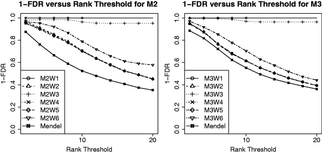
Interaction results of Model 2 and Model 3 under 6 W matrix specifications and Mendel analysis

In comparing our method with that of Wu et al. (2009), as implemented in Mendel, we can see in Figure 3 that our method outperforms stage-wise selection for all choices considered for the matrix W. This observation is significant in showing that using accurate prior information, even with moderate ‘noise’ (i.e. specifying non-existent interactions), it is possible to outperform the stage-wise approach by over 10–20% on the 1 − FDR scale. Note that we used the default option in Mendel that tests interactions among selected main effects. There are other options in Mendel one can choose that may perform somewhat better.

With respect to the detection of main effects, the performance of our methodology is shown in Table 1. The average power of main effects are grouped into three categories: the true SNPs involved in interaction, true SNPs not involved in interaction and the SNPs that have no effect on the simulated trait. Recall that there is no interaction in Model 1, and all true SNPs in Model 3 are involved in interaction, so they have only two relevant groups of SNPs. As we can see from the Model 2 result, SNPs involved in interactions are detected more easily than SNPs not involved in interactions. Comparing Table 1 with Table 2, we can also see that our method has the same or higher average power for detecting true main effects than the stage-wise approach of Wu et al. (2009), as implemented in Mendel. In both approaches, the non-active SNPs have a small chance of being declared as main effects.

Table 1.

Simulation results for detection of main effects

Main effects
	Model 1
SNPs with interaction	—	—	—	—	—	—
SNPs without interaction	0.618	0.645	0.616	0.645	0.645	0.636
Non-active SNPs	0.013	0.012	0.013	0.012	0.012	0.012
	Model 2
SNPs with interaction	1.000	1.000	1.000	1.000	1.000	1.000
SNPs without interaction	0.565	0.607	0.565	0.607	0.606	0.595
Non-active SNPs	0.011	0.011	0.012	0.011	0.011	0.011
	Model 3
SNPs with interaction	1.000	1.000	1.000	1.000	1.000	1.000
SNPs without interaction	—	—	—	—	—	—
Non-active SNPs	0.005	0.005	0.005	0.005	0.005	0.005

Table 2.

Detection of main effects by stage-wise competitor

Main effects	Model 2	Model 3
SNPs with interaction	1.000	1.000
SNPs without interaction	0.557	—
Non-active SNPs	0.012	0.005

We also tested two more cases where main-effect sizes were moderate and weak, corresponding to 50% power and 20% power, respectively, under standard single-SNP additive models. To assess the performance of our method in finding interactions under these various strengths of main effects, we reverse the direction of interactions so that there are no marginal SNP effects. The W matrix we used is , as described before, to make a fair comparison with respect to the inclusion of noise interactions. The results under such models are shown in Figure 4. As we can see from the figure, the approach implemented using Mendel could not find true interactions under any of the models [the regular (Mendel), the moderate (Mendel.moderate) and the weak (Mendel.weak) main-effect models], as it only searches for interactions among main effects selected in the first stage. In contrast, our proposed approach is able to find some of the true interactions because it incorporates information from the W matrix, the network of interactions built from outside knowledge. Not surprisingly, the model with stronger main effect (M2W2, M3W2) performs better in finding true interactions than moderate (M2W2.moderate, M3W2.moderate) or weak (M2W2.weak, M3W2.weak) main-effect models.

Fig. 4.

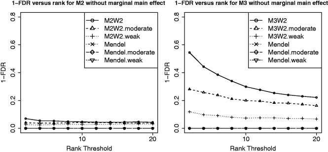
Interaction results of Model 2 and Model 3 without marginal main effect

There are a number of other important questions that one can explore in simulations. We further checked four of them and found that (i) our approach outperforms simple association tests; (ii) scaling up data size by adding more ‘noise’ SNPs makes it harder to find true main effects but does not adversely affect the selection of interactions’ (iii) besides the obvious advantage of decreasing computing time, using network information in our penalty yields advantages in detecting interactions beyond that deriving from the hierarchical nature of the penalty; and (iv) our approach is robust to modest linkage disequilibrium among SNPs. A detailed description of these results can be found in Supplementary Material, Section 4.

4 APPLICATION TO IGE CONCENTRATION

We applied our algorithm to evaluate G × G interactions for log plasma IgE concentration, a biomarker that is often elevated in individuals with allergy to environmental allergens. An elevated plasma IgE concentration is associated with allergic diseases, including asthma, allergic rhinoconjunctivitis, atopic dermatitis and food allergy. Although several genes influencing IgE concentrations have been identified to date, the interactions among these genes or others yet to be identified to be important players have not been studied (Granada et al., 2012).

We sought to investigate G × G effects on log IgE concentration in the FHS cohorts. Participants from the town of Framingham, Massachusetts, have been recruited in these studies starting in 1948, and have been followed over the years for the development of heart disease and related traits, including pulmonary function and allergic response measured by IgE concentration. Our analyses include 6975 participants, 441 from the original cohort recruited in 1948, an additional 2848 from the Offspring cohort recruited in 1971 and finally 3686 participants from the Third Generation cohort initiated in 2002. A recent GWAS on Framingham participants identified new genetic loci associated with plasma total IgE concentrations (Granada et al., 2012). We are interested in looking at G × G interactions associated with IgE concentration, as an illustration of our methodology.

4.1 Preliminaries

Genotypes were from Affymetrix 500K and MIPS 50K arrays, with imputation performed using HapMap 2 European reference panel (Li et al., 2010). Dosage genotypes (expected number of minor alleles) were used in our analysis, although the software implementation of the Wu et al. (2009) approach (Mendel) required genotypes to be coded as 0, 1 or 2 and could not handle dosage. Therefore, in our analysis using Mendel, for each individual, we used the genotype with the highest posterior probability at each SNP. We analyze the natural logarithm of plasma total IgE concentrations as our phenotype (i.e. Y), adjusted for smoking status (current, former and amount of life time smoking in terms of pack-years), age, sex and cohort of origin. A total of 6975 participants (3209 men and 3766 women) aged 19 years and older had good-quality genotypes and were included in our analysis. Familial relationship was ignored when applying our algorithm and the Wu et al. (2009) approach, but we subsequently applied linear mixed-effect models to account for familial correlation to obtain estimates of effect sizes.

Some pre-processing was used to select a set of SNPs to include in our analysis. First, we attempted to map each of the 2 411 590 genotyped and imputed SNPs in the dataset to a reference gene containing it. If no such gene was available, then we mapped the SNP to the closest reference gene within 60 kb of the SNP, if available. Otherwise, the SNP was excluded. After establishing this mapping between genes and SNPs, some genes were found to include multiple SNPs. We kept only one SNP for each gene, selecting in each case that SNP most significantly associated with the phenotype, based on a linear mixed-effect regression. As a result, the SNPs in the final dataset have low linkage disequilibrium (correlation) and a unique SNP-to-gene correspondence (additional analyses suggest that our results, reported below, are fairly robust to modest amounts of disequilibrium in these data. See Supplementary Materials, Section 4.4).

The final dataset has 17 025 SNPs/genes. We used the KEGG pathway database to build our W matrix, following the steps described in Section 2. The KEGG pathway database has a total of 72 354 genes and 5268 unique genes, resulting in 479 066 interactions allowed in our W matrix.

4.2 Results

For our analysis on 17 025 SNPs, we chose to look for 10 main effects, although we allowed the algorithm to terminate after selecting 10 ± 1 main effects, resulting in 9 main effects selected in the current analysis. The parameter c was set to 0.1, which, based on an average estimated SNP variance of 0.27 for these data, corresponds to . Nine interactions were found in our approach, yielding a model with variables. To calibrate our results with those from the stage-wise procedure of Wu et al. (2009), as implemented in Mendel, the latter was run to select 9 variables in the first stage (i.e. fitting only main effects), and then 15 variables in the second stage (i.e. fitting both main effects and interactions, selected from among the 9 SNPs resulting from the first stage). This process produced a final model with nine main effects and six interactions. In terms of computing time, our analysis ran in ∼5 min on our cluster Linga, equipped with two Intel Xeon CPUs E5345 @ 2.33 GHz, with four cores each, and 16 GB/32 GB of RAM for each node (the job was submitted to one node and used one core), while the analysis in Mendel ran in ∼2 min. Given that our method evaluates times more potential interactions than Mendel, the observed trade-off between computing time and number of possible interactions being evaluated appears to be reasonable.

The results from our proposed method and from the stage-wise procedure are shown in the left and right, respectively, of Table 3. The estimates of effect size and the ranks are from the linear mixed-effect model for the final model after variable selection procedure, for both methods. Genes previously found in a GWAS of these FHS data (Granada et al., 2012) are indicated with an asterisk in the table. In our approach, four of the six interaction pairs involved human leukocyte antigen (HLA) genes, which encode antigen-presenting cell-surface proteins that are key regulators of the immune response. The other two interactions identified were among genes both previously associated with log IgE concentrations (Granada et al., 2012). In contrast, Mendel did not detect any interactions among genes in the HLA regions or among pairs of previously associated genes.

Table 3.

Results of application to IgE concentration data

Network-guided sparse regression				Mendel analysis
Gene 1	Gene 2	t-value	Found	Gene 1	Gene 2	t-value	Found
FCER1A		−5.6441	a	LRP1		4.7084
MPP6		4.4184		SNF1LK2		4.3969
STAT6		−4.2453	a	EMID2		−4.1795
IL-13		4.0073	a	RAB3C		3.8585
LRP1		3.7072		HLA-DQA2		3.6883	a
HLA-DPB1	HLA-DQA2	1.6314		FCER1A		−2.8098	a
FCER1A	HLA-DQA2	1.4193		HLA-DPB1		2.1346
HLA-G		1.3657	a	LOC441108		1.9687
HLA-DPB1		1.1655		LOC441108	DDX1	1.7449
HLA-A		0.8442	a	LRP1	DDX1	−1.6417
FCER1A	IL-13	0.6318		FCER1A	SNF1LK2	−1.5967
HLA-DQA2		0.4590	a	DDX1	SNF1LK2	−1.4047
HLA-A	HLA-DPB1	0.4318		DDX1		−1.1802
HLA-G	HLA-A	−0.2813		HLA-DPB1	EMID2	0.8505
HLA-G	HLA-DQA2	0.0678		HLA-DPB1	LOC441108	−0.8076

Note: Terms are ranked based on absolute t-value. ^aThe genes that were found in publication.

From a biological perspective, a number of the interactions discovered by our method are of non-trivial potential interest. The major histocompatibility complex (MHC) class I antigens HLA-A, -B and -C are involved with cell-mediated immunity targeting cells expressing proteins produced intracellularly, for example, by viruses, while the MHC class II antigens HLA-DP, -DQ and -DR play key roles with humoral immunity, including the production of IgE antibodies directed against environmental allergens (Klein and Sato, 2000). HLA-G is a non-classical MHC class I antigen that may have immunomodulatory effects through actions on natural killer cells, T lymphocytes and antigen-presenting cells (Carosella et al., 2008). Genetic variants in these different classes of HLA genes—each class influencing a different but interconnected aspect of immune function—could well interact to influence the risk of developing IgE dysregulation and allergy. The observed interaction between SNPs in the alpha chain of the high affinity receptor for IgE (FCER1A) and interleukin (IL)-13 genes may reflect a number of mechanisms. For example, a genetic variant causing increased expression of FcRI on mast cells would lead to increased antigen-induced activation of these cells, which would consequently produce more IL-13 (Burd et al., 1995), leading to more class-switch recombination and IgE production. Genetic variation of FcRI on classical antigen-presenting cells may also promote Th2 cell activation (Potaczek et al., 2009) with consequent IL-13 release. Thus, SNPs in these two genes in the same pathway leading to increased IgE production could have synergistic effects. Overall, identification of these interactions may help identify the children at highest risk for developing allergy, possibly helping focus interventions to prevent allergy, and may provide new insights into the genetic basis and mechanisms of allergy.

5 DISCUSSION

There are many potential sources of missing hereditability. G × G interactions is one such source. In turn, there are many types of genetic interactions, including multiplicative and non-multiplicative (Mukherjee et al. 2008, 2012). In this article, we focus on investigating multiplicative interactions in the form of a product between two variables. Our proposed methodology provides a promising new approach to tapping this source, by exploiting the wealth of biological knowledge accumulated in various pathway databases.

The simulations reported here suggest that our approach performs better in finding true interactions with a reasonable prior biological knowledge incorporated, compared with the stage-wise regression method that first fits a main-effect model and then searches for interactions among selected main effects. Furthermore, the real-data results are promising in suggesting that better performance likely may be realized in real data as well.

Future work to be done on this topic includes extending the computational algorithm to account for linkage disequilibrium among SNPs, and producing a software implementation that uses standard formatted files such as genotype files from the PLINK (Purcell et al. 2007) software package.

Funding: National Institute Health (grants DK078616, ES020827 GM078987, AG028321, N01 HC25195 and P01 AI050516) (in part). A portion of this research used the Linux Cluster for Genetic Analysis (LinGA-II), funded by the Robert Dawson Evans Endowment of the Department of Medicine at Boston University School of Medicine and Boston Medical Center.

Conflict of Interest: none declared.

REFERENCES

- Ayers K, Cordell H. SNP selection in genome-wide and candidate gene studies via penalized logistic regression. Genet. Epidemiol. 2010;34:879–891. doi: 10.1002/gepi.20543. [DOI] [PMC free article] [PubMed] [Google Scholar]
- Bühlmann P, Van De Geer S. Statistics for High-Dimensional Data: Methods, Theory and Applications. Springer-Verlag New York Inc; 2011. [Google Scholar]
- Burd P, et al. Activated mast cells produce interleukin 13. J. Exp. Med. 1995;181:1373–1380. doi: 10.1084/jem.181.4.1373. [DOI] [PMC free article] [PubMed] [Google Scholar]
- Carosella E, et al. Hla-g: from biology to clinical benefits. Trends Immunol. 2008;29:125–132. doi: 10.1016/j.it.2007.11.005. [DOI] [PubMed] [Google Scholar]
- Friedman J, et al. Pathwise coordinate optimization. Ann. Appl. Stat. 2007;1:302–332. [Google Scholar]
- Granada M, et al. A genome-wide association study of plasma total ige concentrations in the framingham heart study. J. Allergy Clin. Immunol. 2012;129:840–845. doi: 10.1016/j.jaci.2011.09.029. [DOI] [PMC free article] [PubMed] [Google Scholar]
- He Q, Lin D. A variable selection method for genome-wide association studies. Bioinformatics. 2011;27:1. doi: 10.1093/bioinformatics/btq600. [DOI] [PMC free article] [PubMed] [Google Scholar]
- Hindorff L, et al. A catalog of published genome-wide association studies. National Human Genome Research Institute. 2010 http://www. genome. gov/gwastudies. [Google Scholar]
- Klein J, Sato A. The HLA system. First of two parts. N Eng. J. Med. 2000;343:702–709. doi: 10.1056/NEJM200009073431006. [DOI] [PubMed] [Google Scholar]
- Lange K, et al. Mendel version 4.0: a complete package for the exact genetic analysis of discrete traits in pedigree and population data sets. Am. J. Hum. Genet. 2001;69:504. [Google Scholar]
- Li Y, et al. Mach: using sequence and genotype data to estimate haplotypes and unobserved genotypes. Genet. Epidemiol. 2010;34:816–834. doi: 10.1002/gepi.20533. [DOI] [PMC free article] [PubMed] [Google Scholar]
- Logsdon B, et al. A variational Bayes algorithm for fast and accurate multiple locus genome-wide association analysis. BMC Bioinformatics. 2010;11:58. doi: 10.1186/1471-2105-11-58. [DOI] [PMC free article] [PubMed] [Google Scholar]
- Ma S, et al. Identification of non-Hodgkin’s lymphoma prognosis signatures using the CTGDR method. Bioinformatics. 2010;26:15. doi: 10.1093/bioinformatics/btp604. [DOI] [PMC free article] [PubMed] [Google Scholar]
- Manolio T, et al. Finding the missing heritability of complex diseases. Nature. 2009;461:747–753. doi: 10.1038/nature08494. [DOI] [PMC free article] [PubMed] [Google Scholar]
- Mukherjee B, et al. Tests for gene-environment interaction from case-control data: a novel study of type i error, power and designs. Genet. Epidemiol. 2008;32:615–626. doi: 10.1002/gepi.20337. [DOI] [PubMed] [Google Scholar]
- Mukherjee B, et al. Testing gene-environment interaction in large-scale case-control association studies: possible choices and comparisons. Am. J. Epidemiol. 2012;175:177–190. doi: 10.1093/aje/kwr367. [DOI] [PMC free article] [PubMed] [Google Scholar]
- Potaczek D, et al. Genetic variability of the high-affinity ige receptor α-subunit (fcεriα) Immunol. Res. 2009;45:75–84. doi: 10.1007/s12026-008-8042-0. [DOI] [PubMed] [Google Scholar]
- Purcell S, et al. Plink: a toolset for whole-genome association and population-based linkage analysis. Am. J. Hum. Genet. 2007;81:559–575. doi: 10.1086/519795. (Software PLINK v1.07) http://pngu.mgh.harvard.edu/purcell/plink/ [DOI] [PMC free article] [PubMed] [Google Scholar]
- Radchenko P, James G. Variable selection using adaptive nonlinear interaction structures in high dimensions. J. Am. Stat. Assoc. 2010;105:1541–1553. [Google Scholar]
- Szymczak S, et al. Machine learning in genome-wide association studies. Genet. Epidemiol. 2009;33(Suppl. 1):S51–S57. doi: 10.1002/gepi.20473. [DOI] [PubMed] [Google Scholar]
- Wu J, et al. Screen and clean: a tool for identifying interactions in genome-wide association studies. Genet. Epidemiol. 2010;34:275–285. doi: 10.1002/gepi.20459. [DOI] [PMC free article] [PubMed] [Google Scholar]
- Wu T, Lange K. Coordinate descent algorithms for lasso penalized regression. Annals. 2008;2:224–244. [Google Scholar]
- Wu T, et al. Genome-wide association analysis by lasso penalized logistic regression. Bioinformatics. 2009;25:714. doi: 10.1093/bioinformatics/btp041. [DOI] [PMC free article] [PubMed] [Google Scholar]
- Zhou H, et al. Association screening of common and rare genetic variants by penalized regression. Bioinformatics. 2010;26:2375. doi: 10.1093/bioinformatics/btq448. [DOI] [PMC free article] [PubMed] [Google Scholar]