Heat waves in the United States: definitions, patterns and trends

Abstract

High temperatures and heat waves are related but not synonymous concepts. Heat waves, generally understood to be acute periods of extreme warmth, are relevant to a wide range of stakeholders because of the impacts that these events have on human health and activities and on natural environments. Perhaps because of the diversity of communities engaged in heat wave monitoring and research, there is no single, standard definition of a heat wave. Experts differ in which threshold values (absolute versus relative), duration and ancillary variables to incorporate into heat wave definitions. While there is value in this diversity of perspectives, the lack of a unified index can cause confusion when discussing patterns, trends, and impacts. Here, we use data from the North American Land Data Assimilation System to examine patterns and trends in 15 previously published heat wave indices for the period 1979–2011 across the Continental United States. Over this period the Southeast region saw the highest number of heat wave days for the majority of indices considered. Positive trends (increases in number of heat wave days per year) were greatest in the Southeast and Great Plains regions, where more than 12 % of the land area experienced significant increases in the number of heat wave days per year for the majority of heat wave indices. Significant negative trends were relatively rare, but were found in portions of the Southwest, Northwest, and Great Plains.

1 Introduction

As mean global temperatures rise (IPCC 2007), there has been increased attention to the frequency of heat extremes and their social and environmental impacts. In 2012 alone, the Intergovernmental Panel on Climate Change (IPCC) issued the full text of their Special Report on Managing the Risks of Extreme Events and Disasters to Advance Climate Change Adaptation (SREX), the Natural Resources Defense Council (NRDC) released the report “Killer Summer Heat: Projected Death Toll from Rising Temperatures in America Due to Climate Change”, and Climate Communications released the report, “Heat Waves and Climate Change.” These studies provide assessments of recent patterns and trends in heat extremes. They also address the complexities involved in evaluating and projecting the frequency and intensity of heat extremes in a changing climate. The occurrence of multiple high profile extreme heat waves in recent years (e.g., Chicago in 1995, Europe in 2003, Russia in 2010) has highlighted the importance of understanding and projecting patterns in extreme heat anomalies.

With respect to recent trends, the IPCC SREX cites the work of Trenberth et al. (2007) and Alexander et al. (2006), who found that 70–75 % of global land area with data coverage saw a statistically significant increase in minimum temperatures (T_min), while 40–50 % of global land area experienced an increase in maximum temperatures (T_max) over the period 1951–2003. However, Alexander et al. (2006) shows that some regions departed from these trends, two of which were the eastern United States and central North America. In these regions, negative trends in T_min and T_max were observed, supporting Pan et al. (2004) who termed the phrase “warming hole” over this region. In parallel, a number of studies have looked specifically at trends in heat wave events rather than in temperature means (e.g., Meehl and Tebaldi 2004; Hansen et al. 2012). The recent work in Hansen et al. (2012) describes that future (warmer) climates will experience the emergence of a new category of extreme outliers (>3σ over the mean). During the baseline period of 1951–1980, heat wave events classified as >3σ over the mean, covered only 1 % of landmass. However, in recent years (2006–2011) the average landmass coverage of these extreme outliers has been 10 %. Model results from Meehl and Tebaldi (2004) show that heat waves will become more intense, more frequent and longer lasting in the second half of the 21st century.

Trends in T_min and T_max are related, but not necessarily synonymous with trends in heat wave events. In part this is due to the inherent difference between temperature, typically evaluated as a continuous variable, and a heat wave event, understood as an exceedance of some defined threshold. However, it is also a product of the fact that there is no consensus on the definition of a heat wave. While a heat wave is generally understood to be a period of extreme and unusual warmth, quantitative definitions of heat waves differ in (1) the metric of heat used—e.g., daily mean temperature (T_mean) (Anderson and Bell 2011), daily T_max (Peng et al. 2011; Meehl and Tebaldi 2004), temperature and humidity (Grundstein et al. 2012; Rothfusz and Scientific Services Division 1990) and apparent temperature (Steadman 1984)—(2) the manner in which thresholds of exceedence are defined—as an absolute threshold (e.g., T_max greater than 40.6 °C (Robinson 2001)), or as a relative threshold, (e.g., the 95th percentile (Anderson and Bell 2011))—and/or (3) the role of duration in a heat wave definition (e.g., 1 day (Tan et al. 2007), or multiple length criteria (Meehl and Tebaldi 2004).

The diversity of definitions reflects the diversity of reasons that heat waves are studied. Climate scientists, who are primarily interested in the evolving statistics of weather in climate change, tend towards definitions that include a probability of exceedance in some relatively straightforward metric, usually defined relative to a long term mean (e.g., Hansen et al. 2012; Schar et al. 2004). Health researchers, in contrast, are interested in the aspects of a heat wave that are most relevant to human well-being. These heat wave definitions are also more likely to be regionally specific than climate-focused definitions, and may also target vulnerable subsets of the population. These health definitions are often informed by recognized links between heat and morbidity or mortality (Semenza et al. 1999; Hajat et al. 2006; Medina-Ramon and Schwartz 2007; Anderson and Bell 2009), which makes it possible to select or customize heat wave indices for the purpose of predicting health impacts in specific geographic settings or in particular populations (Barnett et al. 2010; Metzger et al. 2010; Williams et al. 2012). Such studies can inform the use of heat wave indices in operational warning systems.

Because of the diversity of stakeholders involved in the study of heatwaves, researchers and health experts are able to collaborate to evaluate local health risks posed by climate variability and change. However, the diversity of definitions can also lead to some confusion in the broader discussion of climate trends and the impacts of climate change. Indices that give a high weight to daily T_max may be higher in hot, dry regions while those focused on daily T_min or apparent temperature would tend to be higher in humid zones. There is value in monitoring and projecting each of these kinds of heat extremes, but there is also a need to be clear about definitions such that reported patterns and trends can be understood in the context of other studies.

In this paper we analyze geographic patterns and trends for the Continental United States (CONUS) in fifteen different previously published heat wave indices (HI). The objective is to describe and explain how the choice of definition influences conclusions regarding the observed frequency of extreme heat events in different regions of the CONUS over the past 33 years, in order to provide a baseline for interpreting studies that project future trends in extreme heat events.

2 Materials and methods

2.1 Data

The meteorological data used in this study are from Phase 2 of the North American Land Data Assimilation System (NLDAS-2). The NLDAS-2 data have a spatial resolution of 1/ 8 degree (~12.5 km) and an hourly temporal resolution (Xia et al. 2012; Mitchell et al. 2004). As heat waves are the focus of this study, only data from the warm season, May 1–Sept 30, were considered. The analysis period is 1979–2011.

NLDAS-2 was used for this study because it provides the most reliable, spatially complete dataset of its kind. The six NLDAS-2 forcing fields used were temperature, surface pressure, specific humidity, downward shortwave radiation, U-wind and V-wind. From these fields, wind speed, net extra radiation per unit area of body surface, relative humidity and vapor pressure were derived.

NLDAS-2 forcing fields are derived from the National Centers for Environmental Prediction (NCEP) North American Regional Reanalysis (NARR) data. NARR fields have a 32 km spatial resolution and 3-hourly temporal resolution. The NARR fields are derived from the 3-hourly NCEP Eta Data Assimilation System (EDAS) when available (~92 % of the time), otherwise the 3-hourly and 6-hourly Eta mesoscale model forecast fields are used (Cosgrove et al. 2003). The NARR assimilation system is fully cycled including prognostic land states with a 3-hourly forecast from the previous cycle serving as a first guess for the next cycle (Mesinger et al. 2006). Additional information about the NARR field processing can be found in Mesinger et al. (2006).

The NLDAS processing system performs a spatial interpolation to downscale NARR fields to the NLDAS 0.125° grid. For all fields used in this study, a bilinear interpolation procedure is used. This interpolation method conserves the area-averaged values, while simultaneously allowing for interpretation to a higher resolution grid (Cosgrove et al. 2003). Following this, a temporal interpolation is performed to adjust to the NLDAS hourly resolution. Once the other interpolations are completed, Geostationary Operational Environmental Satellite (GOES) based shortwave radiation data are used to produce that NLDAS forcing fields (Cosgrove et al. 2003).

The topography of the NLDAS 12.5 km grids is different from the NARR 32 km grids, and therefore temperature, pressure, humidity and longwave radiation fields must be adjusted. First, a lapse rate of −6.5 Kkm⁻¹ is applied to adjust temperature over the change in elevation. Using the adjusted temperature, the 2 m pressure fields are adjusted using the Hydrostatic Approximation and Ideal Gas Law. Specific humidity fields are adjusted by assuming constant relative humidity across the change in elevation, as well as the equations of state for water vapor and dry air, the definition of specific humidity and Wexler’s saturated water vapor pressure equation. Downward longwave radiation is adjusted using the Stefan Boltzman law.

Further details and equations for the interpolations and elevation adjustments can be found in Cosgrove et al. 2003. The implication of the interpolation method for this study is that heat indices defined by absolute thresholds will be responsive to lapse rate corrections, while indices defined using local statistical distributions will be insensitive to the static in time local corrections. We note that for all indices the resolution of NLDAS-2 is appropriate for regional studies but is inadequate to address questions related to urban heat islands, within-municipality variability in extreme heat exposure, or localized effects of contrasts in topography and land cover.

Quality control of the NLDAS-2 forcing fields is based on the Assistance for Land surface modeling Activities (ALMA) forcing data conventions. In addition, validation studies have shown NLDAS forcing fields to be extremely realistic (Cosgrove et al. 2003). One such study focuses on the NLDAS forcing fields validated against in-situ measurements from the Oklahoma Mesonet monitoring network (Luo et al. 2003). The fields of air temperature, surface pressure, specific humidity, downward shortwave and longwave radiation all had an R≥0.92, while wind speed has an R=0.75. Similar validation studies are being completed on NLDAS-2 forcing fields (http://ldas.gsfc.nasa.gov/nldas/NLDAS2valid.php).

2.2 Heat wave indices

Table 1 shows the sixteen, previously published HI used in this study. The indices are divided into two main groups according to the type of threshold used in defining heat wave days: relative thresholds and absolute thresholds. Data from the warm season (1 May–30 September) was used for the years 1979–2011.

Table 1.

Definitions of heat wave indices.

Heat Wave Indices (HI)	Temperature Metric	Threshold	Duration	HI Type	Reference(s)
HI01	Mean daily temperature	>95th percentile	2+ consecutive days	Relative	Anderson and Bell (2011)
HI02	Mean daily temperature	>90th percentile	2+ consecutive days	Relative	Anderson and Bell (2011)
HI03	Mean daily temperature	>98th percentile	2+ consecutive days	Relative	Anderson and Bell (2011)
HI04	Mean daily temperature	>99th percentile	2+ consecutive days	Relative	Anderson and Bell (2011)
HI05	Minimum daily temperature	>95th percentile	2+ consecutive days	Relative	Anderson and Bell (2011)
HI06	Maximum daily temperature	>95th percentile	2+ consecutive days	Relative	Anderson and Bell (2011)
HI07	Maximum daily temperature	T1: >81st percentile T2: >97.5th percentile	Everyday, >T1; 3+ consecutive days, >T2; Avg Tmax>T1 for whole time period	Relative	Peng et al. (2011); Meehl and Tebaldi (2004)
HI08	Maximum daily apparent temperature	>85th percentile	1 day	Relative	Steadman (1984)
HI09	Maximum daily apparent temperature	>90th percentile	1 day	Relative	Steadman (1984)
HI10	Maximum daily apparent temperature	>95th percentile	1 day	Relative	Steadman (1984)
HI11	Maximum daily temperature	>35 °C	1 day	Absolute	Tan et al. (2007)
HI12	Minimum & maximum daily temperature	Tmin>26.7 °C Tmax>40.6 °C	≥1 threshold for 2+ consecutive days	Absolute	Robinson (2001)
HI13	Maximum daily heat index	>80 °F	1 day	Absolute	National Weather Service, Rothfusz and Scientific Services Division (1990); Steadman (1979)
HI14	Maximum daily heat index	>90 °F	1 day	Absolute	National Weather Service, Rothfusz and Scientific Services Division (1990); Steadman (1979)
HI15	Maximum daily heat index	>105 °F	1 day	Absolute	National Weather Service, Rothfusz and Scientific Services Division (1990); Steadman (1979)
HI16*	Maximum daily heat index	>130 °F	1 day	Absolute	National Weather Service, Rothfusz and Scientific Services Division (1990); Steadman (1979)

^*HI16 did not have enough data to include in this analysis.

2.2.1 Relative thresholds

All relative threshold heat indices use the climatological mean over the 1979–2011 time period to calculate the percentiles.

Indices HI01 through HI06 are drawn from Anderson and Bell (2011). For each, a threshold defined on the basis of the long-term local temperature record must be met for at least two consecutive days. HI01 uses daily T_mean and the 95th percentile as the threshold. HI02, HI03 and HI04 apply the same rule to the 90th, 98th, and 99th percentiles of daily T_mean, respectively. HI05 uses the 95th percentile of T_min and HI06 uses the 95th percentile of T_max.

HI07 (Peng et al. 2011; Meehl and Tebaldi 2004) applies a three-step process to define heat wave days. First, for every day in a heat wave the T_max must be over the 81st percentile. Second, the T_max must exceed the 97.5th percentile for at least three consecutive days within the heat wave, but also allowing for days with T_max<97.5th percentile. Lastly, the whole time period classified as a heat wave must have an average T_max greater than the 81st percentile.

HI08, HI09 and HI10 are based on thresholds of Apparent Temperature (AT). Following Steadman (1984), AT is calculated as:

$$AT=-1.8+1.07T+2.4VP-0.92v+0.044Q_g$$ (1)

where AT is measured in °C, T is temperature in °C, VP is vapor pressure in kPa, v is wind speed in ms⁻¹, and Q_g is net extra radiation per unit area of body surface in Wm ⁻². AT is calculated every hour throughout the day, and then daily AT_max is classified into one of three categories: hot (>85th percentile), very hot (>90th percentile) and extremely hot (>95th percentile).

2.2.2 Absolute thresholds

HI11 uses a straightforward approach: everyday that T_max is over 35 °C is classified as a heat wave day (Tan et al. 2007).

HI12 (Robinson 2001) uses both T_min and T_max to define heat wave days: the threshold value for T_max is 40.6 °C and for T_min is 26.7 °C. At least one of these thresholds must be met on at least two consecutive days to classify each of those days as a heat wave day.

HI13 through HI16 use the National Weather Service’s (NWS) heat index (I_NWS). I_NWS is calculated using temperature and relative humidity, however other factors such as vapor pressure, wind speed, characteristics of human activity levels, sweating rate etc. were used to parameterize the equation (Rothfusz and Scientific Services Division 1990). The heat index is calculated using Eq. 2:

$$\begin{array}{l}{I}_{\mathit{NWS}}=-42.379+2.04901523T+10.14333127R-0.22475541TR\\ -0.00683783T^2-0.05481717R^2+0.00122874T^{2}R+0.00085282T^2{R}^2\\ -0.00000199T^2{R}^2\end{array}$$ (2)

where I_NWS is the heat index in °F, T is the temperature in °F and R is relative humidity measured as a percentage (Rothfusz and Scientific Services Division 1990; Steadman 1979). I_NWS is calculated at each hour throughout the day, and then the daily maximum I_NWS is classified into one of four categories: 1) Caution: >80 °F [HI13], 2) Extreme Caution: >90 °F [HI14], 3) Danger: >105 °F [HI15] and 4) Extreme Danger: >130 °F [HI16].

There are two instances where an adjustment is made to the calculation of I_NWS (http://www.hpc.ncep.noaa.gov/heat_index/hi_equation.html). First, if R is less than 13 % and T is between 80 °F and 112 °F, then the following adjustment value is subtracted:

$$\frac{13-R}{4}\ast \sqrt{\frac{17-\mid T-95\mid }{17}}$$ (3)

Second, if R is greater than 85 % and T is greater than 80 °F but less than 87 °F, then the following adjustment value is added:

$$\frac{R-85}{10}\ast \frac{87-T}{5}$$ (4)

The highest threshold value, HI16, was too rare to inform statistical analyses of frequency or trends. Because of this, HI16 results will not be shown.

2.3 Statistical Analysis

For each HI, the number of heat wave days was summed annually (warm season) at the NLDAS grid cell scale. To gain insight into regionalized patterns of the HI, CONUS was divided into six regions: Northwest (Washington, Oregon, Idaho), Southwest (California, Nevada, Utah, Arizona, New Mexico and Colorado), Great Plains (North Dakota, South Dakota, Montana, Wyoming, Nebraska, Kansas, Oklahoma, Texas), Midwest (Minnesota, Iowa, Missouri, Wisconsin, Illinois, Indiana, Ohio, Michigan), Southeast (Arkansas, Louisiana, Mississippi, Alabama, Tennessee, Kentucky, Georgia, Florida, South Carolina, North Carolina, Virginia) and Northeast (Pennsylvania, New Jersey, New York, Rhode Island, Connecticut, Massachusetts, Vermont, New Hampshire, Maine, Maryland, West Virginia, Delaware). These regions are depicted in Figure 1 and approximately match the six geographical regions used for regional climate change analysis in the United States Global Change Research Program (USGCRP) report Global Climate Change Impacts in the United States (2009).

Fig. 1.

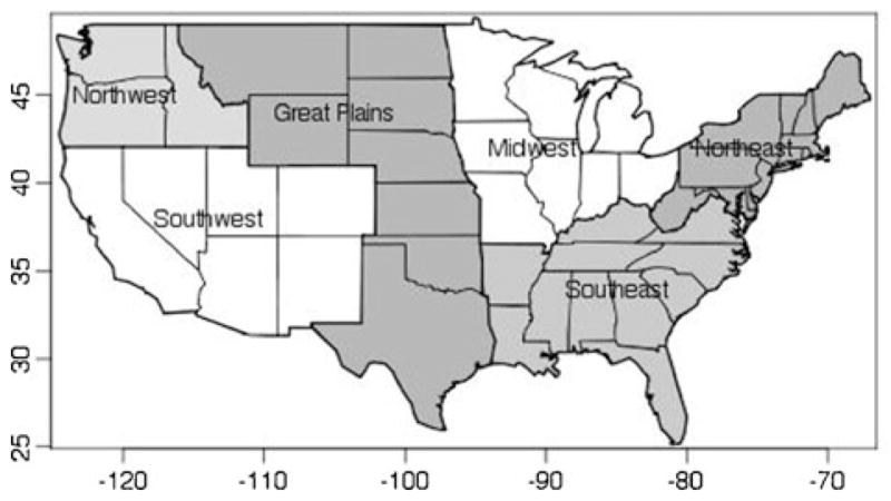
Regional division of the Continental United States (CONUS)

For each of the fifteen HI, the total number of annual heat wave days was averaged over the 33-year timespan at the NLDAS grid cell scale. These results were then averaged over the six CONUS regions to arrive at the average number of heat wave days unique for each heat wave index and region.

These heat wave day averages were then assessed for their trends over the 1979–2011 time period using ordinary least squares (OLS) regression. As the OLS residuals exhibited non-normality for several indices (as shown by Shapiro-Wilks normality testing), significance tests were performed using the Mann-Kendall tau test. The Mann-Kendall tau test is a nonparametric test that does not assume an underlying probability distribution of the data, and is also robust to outliers (Moberg et al. 2006). Because of this, it is valuable when assessing trends in climate data and therefore has been used in previous studies of trends in extreme temperature indices (El Kenawy et al. 2011; Efthymiadis et al. 2011; Kuglitsch et al. 2010). A trend was considered statistically significant if the p-value was smaller than the significance level α of 0.05. Based on the results of the Mann-Kendall testing, all insignificant trends were masked out. The average of the resulting significant trends was computed for each of the six CONUS regions for all fifteen HI. Results are reported for trends calculated over the entire 1979–2011 period of record available at the time the study was performed. The sensitivity of trends to choice of time period was assessed by repeating the trend analysis with the beginning date shifted between 1979 and 1981 and the end date shifted between 2007 and 2012 (provisional data used for 2012). It was found that results were very similar for all analyses that included data through at least 2009. For periods that excluded recent years the geographic pattern and direction of trends was similar, but statistical significance of trends tended to be reduced.

To compliment these trend values, landmass coverage was calculated. These landmass coverage percentages represent the number of cells covered by significant trends (which were averaged) divided by the total number of cells in that region.

3 Results

To provide an example of the prevailing climate characteristics used to define the relative HI, Fig. 2 shows the average daily T_max, standard deviation of the daily T_max, and the 95th percentile threshold for T_max for May–September 1979–2011. That is to say, for HI06 the temperature field mapped in Fig. 2c must be met for at least two consecutive days for those days to count as a heat wave day.

Fig. 2.

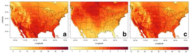
a Average daily T_max (°C) over the time period 1979–2011. b Standard deviation of T_max over the time period 1979–2011. c 95th percentile of T_max(°C)

3.1 Average annual heat wave days

Figure 3 shows the results of the analysis of the average number of annual heat wave days; note that scale bars differ depending on the definition so as to accentuate the spatial patterns. To get a quantitative look at these differences, Table 2 shows the results of this analysis for each of the six CONUS regions.

Fig. 3.

1979–2011, annual average number of heat wave days. Note the varying scales. Results for HI01–HI15 are shown by a–o, respectively

Table 2.

Average number of annual heat wave days, divided by region.

	NW	SW	GP	MW	SE	NE
HI01	3.92	1.54	2.23	2.73	1.76	2.56
HI02	11.95	7.77	8.82	9.39	7.00	9.79
HI03	0.77	0.16	0.30	0.54	0.26	0.30
HI04	0.24	0.05	0.07	0.15	0.06	0.05
HI05	3.92	1.45	1.44	1.97	0.21	2.02
HI06	3.42	1.96	3.12	3.73	4.59	2.71
HI07	0.50	0.27	0.78	1.42	2.26	0.49
HI08	22.53	20.01	20.98	21.54	21.08	21.72
HI09	12.47	9.90	11.01	12.09	12.13	11.96
HI10	3.60	2.23	2.89	3.76	3.94	3.53
HI11	2.25	21.76	23.06	3.80	6.76	0.16
HI12	0.10	5.94	4.48	0.46	4.49	0.01
HI13	4.00	15.92	52.93	58.75	113.63	28.54
HI14	0.23	2.04	23.58	26.48	72.10	7.61
HI15	0.00	0.16	1.29	2.35	4.66	0.17

Bold indicates region with highest frequency of heat waves days for each HI.

Regions are: Northwest (NW), Southwest (SW), Great Plains (GP), Midwest (MW), Southeast (SE) and Northeast (NE).

The Northwest region experienced the highest frequency of heat wave occurrence for HI01–HI05, HI08 and HI09, the Southeast experienced the highest frequency for HI06, HI07, HI10, HI11, and HI13–HI15 and the Southwest experienced the highest frequency for HI12. The Great Plains, Midwest and Northeast regions did not see the highest frequency of heat wave occurrence for any HI. The range of averages between the six regions was much smaller for relative threshold definitions than the range seen between absolute threshold definitions.

3.2 Temporal trends

Figure 4 shows the results of temporal trend analysis. Only the trends with significance over 95 %, based on the Mann-Kendall test, are shown in color. The majority of the trends are positive, indicating that from 1979 to 2011 the average number of annual heat wave days has increased. Figure 5 summarizes this trend information for defined CONUS regions in terms of magnitude and extent of significant trends. The value printed in each cell is the trend value (in days/year). The color of the cell represents the direction of the trend, where red represents positive trends and blue represents negative trends. The shades of red and blue represent the landmass percentage covered by this significant trend, increasing in percentage from the lightest shades to the darkest shades.

Fig. 4.

Trends in the number of annual heat wave days, over the period 1979–2011. White areas indicate results below 95 % significance. Units are days/year

Fig. 5.

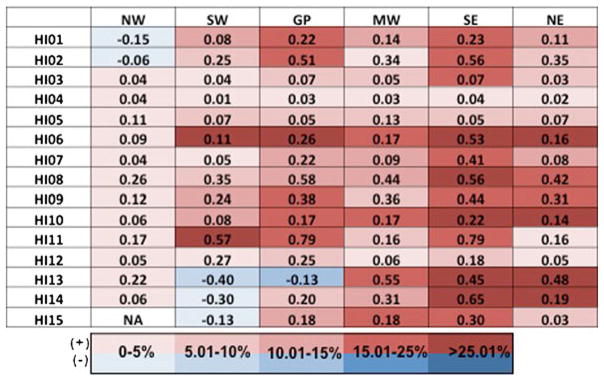
Average 95 % significant trends in the number of annual heat wave days, over the period 1979–2011, divided by region. The value printed in each cell is the trend value (in days/year). The color of the cell represents positive (red) and negative (blue) trends. The shades of red and blue represent the landmass percentage covered by this significant trend given by the scale bar. Regions are: Northwest (NW), Southwest (SW), Great Plains (GP), Midwest (MW), Southeast (SE) and Northeast (NE)

The majority of the trends observed across CONUS regions are positive, with the largest positive trends found in the Southeast and Great Plains regions. For the positive trends, the percentage of landmass covered ranges from 0 % to 38 %. Positive trends were found across more than 12 % of the landmass area for the majority of HI for the Southeast and Great Plains regions; coverage over 12 % was found for twelve HI in the Southeast and eight indices in the Great Plains. The largest magnitude negative trend was found in the Southwest region, with other negative trends seen in the Northwest and Great Plains regions. Landmass coverage of these negative trends ranged from 0 % to 12 %.

4 Discussion

The results of the index intercomparison presented in this study are generally consistent with warming trends observed in previous studies (Meehl and Tebaldi 2004; Schar et al. 2004; Hansen et al. 2012). Our study shows that in the past 33 years the frequency of heat waves days has increased across most CONUS regions, according to the majority of HI. Some of our results show regional exceptions to these overall trends: negative trends were found for HI01 and HI02 in the Northwest, HI13 in the Southwest and Great Plains and HI14 and HI15 in the Southwest.

In looking at the frequency of heat wave days over the past 33 years, the geographical patterns are varied between HI. Most of the patterns shown in Fig. 3 have a sensible explanation based on what information was included in the definition of a heat wave day. For example, the geographical patterns of high heat wave day frequency in HI13 and HI14 correspond to the areas of CONUS with high humidity; this is consistent with the fact that these definitions include both temperature and relative humidity data.

Our results do differ from some previous studies of heat wave trends in the United States. These apparent inconsistencies can be attributed to differences in time period of analysis, data source, spatial resolution of analysis, and heat wave definitions. For example, Alexander et al. (2006) found that the Southeast region has experienced a decrease in heat waves, but their study used an earlier time period, 1951–2003, and defined a heat wave on the basis of single day T_max. Robinson (2001) also found decreases in heat waves throughout the US South. That study uses the HI12 definition of a heat wave day, but is based on an earlier time period, 1951–1990, and uses station data that resulted in a coarser temporal resolution. Such discrepancies make it difficult to compare results across studies and can lead to some confusion in assessments of the magnitude and geography of heat wave trends.

The diversity of HI found in the literature is understandable, considering the range of reasons that heat waves are studied. While climate scientists are often concerned with trends in the statistics of high temperature, health experts focus on indices that capture impacts on human well-being, which are frequently influenced by social factors such as acclimation and exposure. Collaboration between climate and health communities is particularly valuable in this context. For example, a number of health-oriented studies have demonstrated that the largest mortality effects due to increased heat occur in northern cities in the United States, or areas with milder summers (Anderson and Bell 2011; Medina-Ramon and Schwartz 2007; Curriero et al. 2002). Here, we find that in the NLDAS record, ten of the fifteen indices show that the percent area experiencing significant increases in heat waves is larger in the Southeast than in the Northeast, and that for nine of these ten indices the magnitude of trend has been greater in the Southeast than the Northeast. Therefore, according to the majority of indices considered in this study the Southeast has seen larger and more spatially extensive trends than the Northeast. Future studies can pair this information with the relative health effects of heat waves in differing regions to grasp a complete understanding for planning health interventions and climate change adaptation strategies. The Northwest region is another example of the potential value in communication across fields: while several of the objective indices in this study had their highest frequency in the Northwest, health experts recognize that heat waves have not been a major health concern in that region relative to other parts of the country.

There are also discrepancies between the research literature and operational health warnings. Davis et al. (2006) found that relative threshold HI are better predictors of health impacts than those that use absolute thresholds. However, HI13–HI16, which use absolute thresholds, are of particular importance to the general public because they align with the heat alerts that are issued by the National Weather Service and broadcast by organizations such as The Weather Channel. In a recent study of US football player deaths, Grundstein et al. (2012) found that 45 % of these deaths occurred in conditions that did not trigger an NWS alert (meaning conditions less than the HI13 threshold). The spatial patterns and trends observed in HI13–HI15 do not align particularly closely with any other HI, which raises the question of whether the public is receiving the most meaningful information regarding heat wave events.

The specific results of our study are limited by the dataset used in the analysis: NLDAS-2 is the preeminent gridded land surface reanalysis for the United States, but it relies on relatively coarse NARR fields as the foundation for meteorological estimates and its downscaling routines do not account for localized differences in lapse rate or surface properties or for nonstationarities such as land-use change. For this reason the patterns and trends identified in this study must be understood as mesoscale results that do not account for phenomena such as urban heat islands that are relevant to local health impacts. In addition, only monotonic trends in heat wave days were considered; higher order trend analysis could provide further insight on recent climate changes. Nevertheless, it is shown that choice of index is critically important to the resulting analysis of patterns and trends. In addition, these index comparisons could be translated easily to different datasets for more focused local analyses.

5 Conclusions

This study demonstrates that estimates of the frequency, trends, and geographical patterns of heat waves in the CONUS strongly depend on how heat waves are defined. This fact, combined with discrepancies between studies in the time period considered, meteorological datasets used, and spatial resolution of analysis, has led to a wide range of conclusions regarding frequency and trends of extreme heat events in the United States.

This study shows that across CONUS regions the range in average number of heat wave days is greater for absolute HI than for relative HI. For both the relative and absolute HI, the Southeast saw the highest values of average heat wave days, indicating that the Southeast has experienced more heat wave days from 1979 to 2011 than any other CONUS region. From the trend analysis, this study has shown that the Southeast and Great Plains regions have experienced both the largest magnitude and most widespread increases in heat wave days per year according to most indices.

Characterization and regionalization of heat waves across the United States is essential to expanding our knowledge of climate change processes and impacts. Understanding the role that definitions play in such studies is important for interpreting seemingly contradictory results and for enhancing the quality of communication between climate scientists, health researchers, and the general public. In this study, we have applied one consistent dataset to compare patterns and trends across fifteen previously published HI. Similar comparisons can be performed for other meteorological datasets and for future climate projections in order to explore the full range of heat wave impacts associated with climate variability and change.

References

- Alexander LV, Zhang X, Peterson TC, Caesar J, Gleason B, Tank A, Haylock M, Collins D, Trewin B, Rahimzadeh F, Tagipour A, Kumar KR, Revadekar J, Griffiths G, Vincent L, Stephenson DB, Burn J, Aguilar E, Brunet M, Taylor M, New M, Zhai P, Rusticucci M, Vazquez-Aguirre JL. Global observed changes in daily climate extremes of temperature and precipitation. J Geophys Res-Atmos. 2006;111:22. [Google Scholar]
- Anderson BG, Bell ML. Weather-related mortality how heat, cold, and heat waves affect mortality in the United States. Epidemiology. 2009;20:205–213. doi: 10.1097/EDE.0b013e318190ee08. [DOI] [PMC free article] [PubMed] [Google Scholar]
- Anderson GB, Bell ML. Heat waves in the United States: mortality risk during heat waves and effect modification by heat wave characteristics in 43 U.S. Communities. Environ Heal Perspect. 2011;119:210–218. doi: 10.1289/ehp.1002313. [DOI] [PMC free article] [PubMed] [Google Scholar]
- Barnett AG, Tong S, Clements ACA. What measure of temperature is the best predictor of mortality? Environ Res. 2010;110:604–611. doi: 10.1016/j.envres.2010.05.006. [DOI] [PubMed] [Google Scholar]
- Cosgrove BA, Lohmann D, Mitchell KE, Houser PR, Wood EF, Schaake JC, Robock A, Marshall C, Sheffield J, Duan QY, Luo LF, Higgins RW, Pinker RT, Tarpley JD, Meng J. Real-time and retrospective forcing in the North American Land Data Assimilation System (NLDAS) project. J Geophys Res-Atmos. 2003;108:12. [Google Scholar]
- Curriero FC, Heiner KS, Samet JM, Zeger SL, Strug L, Patz JA. Temperature and mortality in 11 cities of the eastern United States. Am J Epidemiol. 2002;155:80–87. doi: 10.1093/aje/155.1.80. [DOI] [PubMed] [Google Scholar]
- Davis RE, Knight D, Hondula D, Knappenberger PC. A comparison of biometeorological comfort indices and human mortality during heat waves in the United States. Paper presented at Human biometeorology: The heat 17th conference on biometeorology and aerobiology; San Diego, CA. 2006. Retrieved from https://ams.confex.com/ams/BLTAgFBioA/techprogram/paper_110867.htm. [Google Scholar]
- Efthymiadis D, Goodess CM, Jones PD. Trends in Mediterranean gridded temperature extremes and large-scale circulation influences. Nat Hazard Earth Syst Sci. 2011;11:2199–2214. [Google Scholar]
- El Kenawy A, Lopez-Moreno JI, Vicente-Serrano SM. Recent trends in daily temperature extremes over northeastern Spain (1960–2006) Nat Hazard Earth Syst Sci. 2011;11:2583–2603. [Google Scholar]
- Karl Thomas R, Melillo Jerry M, Peterson Thomas C., editors. Global Climate Change Impacts in the United States. Cambridge University Press; 2009. [Google Scholar]
- Grundstein AJ, Ramseyer C, Zhao F, Pesses JL, Akers P, Qureshi A, Becker L, Knox JA, Petro M. A retrospective analysis of American football hyperthermia deaths in the United States. Int J Biometeorol. 2012;56:11–20. doi: 10.1007/s00484-010-0391-4. [DOI] [PubMed] [Google Scholar]
- Hajat S, Armstrong B, Baccini M, Biggeri A, Bisanti L, Russo A, Paldy A, Menne B, Kosatsky T. Impact of high temperatures on mortality - Is there an added heat wave effect? Epidemiology. 2006;17:632–638. doi: 10.1097/01.ede.0000239688.70829.63. [DOI] [PubMed] [Google Scholar]
- Hansen J, Sato M, Ruedy R. Perception of climate change. Proc Natl Acad Sci U S A. 2012;109:E2415–E2423. doi: 10.1073/pnas.1205276109. [DOI] [PMC free article] [PubMed] [Google Scholar]
- IPCC. Climate Change 2007: the physical science basis. In: Solomon S, Qin D, Manning M, Chen Z, Marquis M, Averyt KB, Tignor M, Miller HL, editors. Contribution of Working Group I to the Fourth Assessment Report of the Intergovernmental Panel on Climate Change. Cambridge University Press; Cambridge, United Kingdom and New York, NY, USA: 2007. p. 996. [Google Scholar]
- IPCC. Managing the risks of extreme events and disasters to advance climate change adaptation. In: Field CB, Barros V, Stocker TF, Qin D, Dokken DJ, Ebi KL, Mastrandrea MD, Mach KJ, Plattner G-K, Allen SK, Tignor M, Midgley PM, editors. A special report of Working Groups I and II of the Intergovernmental Panel on Climate Change. Cambridge University Press; Cambridge, UK, and New York, NY, USA: 2012. p. 582. [Google Scholar]
- Kuglitsch FG, Toreti A, Xoplaki E, Della-Marta PM, Zerefos CS, Turkes M, Luterbacher J. Heat wave changes in the eastern Mediterranean since 1960. Geophys Res Lett. 2010;37:5. [Google Scholar]
- Luo LF, Robock A, Mitchell KE, Houser PR, Wood EF, Schaake JC, Lohmann D, Cosgrove B, Wen FH, Sheffield J, Duan QY, Higgins RW, Pinker RT, Tarpley JD. Validation of the North American Land Data Assimilation System (NLDAS) retrospective forcing over the southern Great Plains. J Geophys Res-Atmos. 2003;108:10. [Google Scholar]
- Medina-Ramon M, Schwartz J. Temperature, temperature extremes, and mortality: a study of acclimatisation and effect modification in 50 US cities. Occupational and Environmental Medicine. 2007;64:827–833. doi: 10.1136/oem.2007.033175. [DOI] [PMC free article] [PubMed] [Google Scholar]
- Meehl GA, Tebaldi C. More intense, more frequent, and longer lasting heat waves in the 21st century. Science. 2004;305:994–997. doi: 10.1126/science.1098704. [DOI] [PubMed] [Google Scholar]
- Mesinger F, DiMego G, Kalnay E, Mitchell K, Shafran PC, Ebisuzaki W, Jovic D, Woollen J, Rogers E, Berbery EH, Ek MB, Fan Y, Grumbine R, Higgins W, Li H, Lin Y, Manikin G, Parrish D, Shi W. North American regional reanalysis. Bulletin of the American Meteorological Society. 2006;87:343–360. [Google Scholar]
- Metzger KB, Ito K, Matte TD. Summer Heat and Mortality in New York City: How Hot Is Too Hot? Environ Heal Perspect. 2010;118:80–86. doi: 10.1289/ehp.0900906. [DOI] [PMC free article] [PubMed] [Google Scholar]
- Mitchell KE, Lohmann D, Houser PR, Wood EF, Schaake JC, Robock A, Cosgrove BA, Sheffield J, Duan QY, Luo LF, Higgins RW, Pinker RT, Tarpley JD, Lettenmaier DP, Marshall CH, Entin JK, Pan M, Shi W, Koren V, Meng J, Ramsay BH, Bailey AA. The multi-institution North American Land Data Assimilation System (NLDAS): Utilizing multiple GCIP products and partners in a continental distributed hydrological modeling system. J Geophys Res-Atmos. 2004;109:32. [Google Scholar]
- Moberg A, Jones PD, Lister D, Walther A, Brunet M, Jacobeit J, Alexander LV, Della-Marta PM, Luterbacher J, Yiou P, Chen DL, Tank A, Saladie O, Sigro J, Aguilar E, Alexandersson H, Almarza C, Auer I, Barriendos M, Begert M, Bergstrom H, Bohm R, Butler CJ, Caesar J, Drebs A, Founda D, Gerstengarbe FW, Micela G, Maugeri M, Osterle H, Pandzic K, Petrakis M, Srnec L, Tolasz R, Tuomenvirta H, Werner PC, Linderholm H, Philipp A, Wanner H, Xoplaki E. Indices for daily temperature and precipitation extremes in Europe analyzed for the period 1901–2000. J Geophys Res-Atmos. 2006;111:25. [Google Scholar]
- Pan ZT, Arritt RW, Takle ES, Gutowski WJ, Anderson CJ, Segal M. Altered hydrologic feedback in a warming climate introduces a “warming hole”. Geophys Res Lett. 2004;31:4. [Google Scholar]
- Peng RD, Bobb JF, Tebaldi C, McDaniel L, Bell ML, Dominici F. Toward a quantitative estimate of future heat wave mortality under global climate change. Environ Heal Perspect. 2011;119:701–706. doi: 10.1289/ehp.1002430. [DOI] [PMC free article] [PubMed] [Google Scholar]
- Robinson PJ. On the definition of a heat wave. J Appl Meteorol. 2001;40:762–775. [Google Scholar]
- Rothfusz LP Scientific Services Division. The heat index “equation” (or, more than you ever wanted to know about heat index) (SR 90-23) 1990 Retrieved from NWS Southern Region Headquarters website: http://www.srh.noaa.gov/images/ffc/pdf/ta_htindx.PDF.
- Schar C, Vidale PL, Luthi D, Frei C, Haberli C, Liniger MA, Appenzeller C. The role of increasing temperature variability in European summer heatwaves. Nature. 2004;427:332–336. doi: 10.1038/nature02300. [DOI] [PubMed] [Google Scholar]
- Semenza JC, McCullough JE, Flanders WD, McGeehin MA, Lumpkin JR. Excess hospital admissions during the July 1995 heat wave in Chicago. American Journal of Preventive Medicine. 1999;16:269–277. doi: 10.1016/s0749-3797(99)00025-2. [DOI] [PubMed] [Google Scholar]
- Steadman RG. Assessment of sultriness.2. Effects of wind, extra radiation and barometric pressure on apparent temperature. J Appl Meteorol. 1979;18:874–885. [Google Scholar]
- Steadman RG. A universal scale of apparent temperature. J Clim Appl Meteorol. 1984;23:1674–1687. [Google Scholar]
- Tan JG, Zheng YF, Song GX, Kalkstein LS, Kalkstein AJ, Tang X. Heat wave impacts on mortality in Shanghai, 1998 and 2003. Int J Biometeorol. 2007;51:193–200. doi: 10.1007/s00484-006-0058-3. [DOI] [PubMed] [Google Scholar]
- Trenberth KE, Jones PD, Ambenje P, Bojariu R, Easterling D, Klein Tank A, Parker D, Rahimzadeh F, Renwick JA, Rusticucci M, Soden B, Zhai P. Observations: surface and atmospheric climate change. In: Solomon S, Qin D, Manning M, Chen Z, Marquis M, Averyt KB, Tignor M, Miller HL, editors. Climate Change 2007: the physical science basis. Contribution of Working Group I to the Fourth Assessment Report of the Intergovernmental Panel on Climate Change. Cambridge University Press; Cambridge, UK: 2007. pp. 237–336. [Google Scholar]
- Williams S, Nitschke M, Sullivan T, Tucker GR, Weinstein P, Pisaniello DL, Parton KA, Bi P. Heat and health in Adelaide, South Australia: assessment of heat thresholds and temperature relationships. Sci Total Environ. 2012;414:126–133. doi: 10.1016/j.scitotenv.2011.11.038. [DOI] [PubMed] [Google Scholar]
- Xia YL, Mitchell K, Ek M, Sheffield J, Cosgrove B, Wood E, Luo LF, Alonge C, Wei HL, Meng J, Livneh B, Lettenmaier D, Koren V, Duan QY, Mo K, Fan Y, Mocko D. Continental-scale water and energy flux analysis and validation for the North American Land Data Assimilation System project phase 2 (NLDAS-2): 1. Intercomparison and application of model products. Journal of Geophysical Research-Atmospheres. 2012;117:27. [Google Scholar]