Encoding of Coordinated Reach and Grasp Trajectories in Primary Motor Cortex

Abstract

Though the joints of the arm and hand together comprise 27 degrees of freedom, an ethological movement like reaching and grasping coordinates many of these joints so as to operate in a reduced dimensional space. We used a generalized linear model to predict single neuron responses in primary motor cortex (MI) during a reach-to-grasp task based on 40 features that represent positions and velocities of the arm and hand in joint angle and Cartesian coordinates as well as the neurons' own spiking history. Two rhesus monkeys were trained to reach and grasp one of five objects, located at one of seven locations while we used an infrared camera motion-tracking system to track markers placed on their upper limb and recorded single-unit activity from a microelectrode array implanted in MI. The kinematic trajectories that described hand shaping and transport to the object depended on both the type of object and its location. Modeling the kinematics as temporally extensive trajectories consistently yielded significantly higher predictive power in most neurons. Furthermore, a model that included all feature trajectories yielded more predictive power than one that included any single feature trajectory in isolation, and neurons tended to encode feature velocities over positions. The predictive power of a majority of neurons reached a plateau for a model that included only the first five principal components of all the features' trajectories, suggesting that MI has evolved or adapted to encode the natural kinematic covariations associated with prehension described by a limited set of kinematic synergies.

Introduction

Reaching and grasping is a complex, ethologically relevant movement. Our earliest primate ancestors developed a mobile forelimb and an opposable thumb to reach and grasp for fruits and insects in the trees (Marzke, 1994). To perform this task, the CNS must coordinate the proximal and distal muscles of the arm and hand to simultaneously bring the hand toward an object's location, rotate the wrist so as to orient the hand with the object and slowly hone in and wrap the fingers around the object. Psychophysics studies have demonstrated that proximal and distal arm movements are coordinated both in time and space during natural reach-to-grasp behaviors and that this coordination is revealed as specific patterns of covariation between reach and grasp trajectories (Haggard and Wing, 1998). Little is known, however, about how the nervous system encodes these coordination patterns.

Several studies, using cortical electrical stimulation and spike-triggered averaging of EMG activity, have shown that there is an overlap between reach and grasp regions in the primary motor cortex (MI) and that single neurons can activate movements about multiple joints involved in a reach-to-grasp movement (Donoghue et al., 1992; McKiernan et al., 1998; Park et al., 2001). MI neurons have been shown to modulate their discharge rates with respect to reach and grasp parameters (Vargas-Irwin et al., 2010), but limited research has investigated how the covarying kinematic patterns of a reach-to-grasp movement are encoded at a single-neuron level. Studies that have examined reaching or grasping in isolation suggest that MI neurons encode these movements as kinematic trajectories that extend in time (Hocherman and Wise, 1991; Saleh et al., 2010; Hatsopoulos et al., 2007). The goal of this study was to extend previous work by developing a detailed, kinematic-based encoding model to characterize how single neurons simultaneously represent hand shaping and transport during a prehensile movement. We used a generalized linear model to estimate the firing rate of single units in 4 ms time bins from a set of reach and grasp kinematics and each neuron's firing history. For a majority of neurons, the predictive power of the encoding model continued to improve as the duration of the kinematic trajectories increased up to ∼350 ms, starting ∼50 ms before the occurrence of a spike. We show that MI is intermingled with neurons that encode reach-related, grasp-related, and combined reach- and grasp-related neurons. Furthermore, encoding models that included all relevant kinematic features instead of just one yielded the highest predictive power for a majority of neurons. We modeled the natural coordination patterns in the reach and grasp kinematics by calculating the principal components (PCs) of the joint kinematic trajectories. For a majority of neurons, the predictive power of the encoding model reached a plateau with just the first five principal components. These results suggest that neurons encode a limited set of spatiotemporal kinematic trajectories that represent the natural motions of the arm and hand in a reach-to-grasp paradigm.

Materials and Methods

Behavioral task.

Two nonhuman primates (female rhesus macaques: monkey O, 6.6 kg; monkey A, 6.5 kg) were trained to reach and grasp objects with their right hand. A trial consisted of four different periods: a premovement period; a reach period preceding the grasp; a hold period when the monkey held the object; and a release period when the robot retracted the object (Fig. 1A). During the premovement period, the experimenter blocked the animal's vision, and the animal rested her hand on a static button while the robot moved the object to the preprogrammed location for the given trial (Fig. 1). The experimenter then retracted the vision blocker, and the animal started to move her hand toward the object to grasp it. Once the object was grasped, the animal was instructed to hold the object until the robot retracted it (∼2 s). Four objects were presented, requiring a total of five hand configurations (Fig. 1B). The first object was a key-like object (a thin, flat object) that elicited a key grip, where the monkey held the object between the thumb and the side of the middle phalanx of the index finger; the second object, the D-ring, was presented twice, in configurations that elicited a whole-hand power grip in two different wrist orientations. These two different configurations will be treated as separate objects—the horizontal D-ring and the vertical D-ring—in the rest of this article. The third object, a sphere, elicited a whole-hand grip with a fanning of the fingers. The fourth object, the small D-ring, elicited a precision grip where the tips of the index and thumb were opposed. These objects were designed to evoke a variety of coordination patterns among the joint angle kinematic trajectories. A robot (RV-1A-S11 6-axis Robot; www.rixan.com) was programmed to place the objects at seven different locations in the monkey's reaching space (Fig. 1C). The object locations were presented in pseudorandom order so that the monkey could not predict the object location on any given trial. Each object was presented to the monkey in a block of at least 140 trials where the seven locations were presented in pseudorandom order.

Figure 1.

Methods. A, Task timeline: at the start of a trial, the monkey rested her hand over a button while the robot moved the object to one of seven locations in the subject's reaching range. After 2 s elapsed, the experimenter pulled a vision block out of the monkey's visual space at which point the monkey was instructed to reach and grasp the object (object presented). The monkey was trained to hold the object until the robot retracted it. After releasing the object, the monkey was instructed to place her hand back on the button. Twenty-three retro-reflective markers were placed on the monkey's arm and fingers. Their 3-D positions were captured with infrared cameras and used to calculate the joint angle kinematics of the arm and hand. B, Five objects were used in the reach-to-grasp task (top to bottom): the key grip, the horizontal D-ring, the vertical D-ring, the sphere, and the small D-ring. C, Seven target locations. Aerial (top) and side view (bottom). D, MI electrode array implants in subject O (left) and subject A (right). Monkey O's array was implanted a little more medially than monkey A's array. The other arrays were used for different studies.

Neural data acquisition.

Each monkey was chronically implanted with a 100-electrode (400 μm interelectrode separation, 1.5 mm electrode length; Blackrock Microsystems) microelectrode array in the arm–hand area of MI in the left hemisphere, contralateral to the hand they used to grasp the objects. The array was placed parallel as close as possible to the central sulcus, medial from the spur of the arcuate sulcus (Fig. 1D). Surgical details have been described previously (Rousche and Normann, 1992; Maynard et al., 1997, 1999). During each recording session, signals were amplified (gain 5000×), bandpass filtered between 0.3 and 7.5 kHz, and digitized at 30 kHz using the Cerebus Neural Data Acquisition system (Blackrock Microsystems). For each channel, a threshold was set above the noise band: if the signal crossed the threshold, a 1.6 ms duration of the signal—so as to yield 48 samples given a sampling frequency of 30 kHz—was sampled around the occurrence of the threshold crossing. To classify the waveforms as noise or units on the given channel, the waveforms were spike sorted off-line using a semiautomated Matlab routine (Mathworks) developed in our laboratory, incorporating some elements of a previously published algorithm (Vargas-Irwin and Donoghue, 2007).

Motion tracking.

The three-dimensional (3-D) positions of monkey's right arm, wrist, hand, and fingers were recorded using a video-based motion analysis system (Vicon Motion Tracking System, Workstation 460). We used six M2 cameras at 1.2 megapixel resolution. Twenty-three spherical retro-reflective markers (3 mm diameter) were glued to the monkeys' fingers, hand, and forearm (Fig. 1A). To compute the inverse kinematics (i.e., the joint angles from the marker positions), we used a scaled version of a skeletal model of the arm (Holzbaur et al., 2005) developed using the OpenSim platform (https://simtk.org/home/opensim). We calculated the following angular positions and velocities: at the shoulder, the three degrees of freedom were rotation about the coronal plane [i.e., variability in abduction/adduction (ELV)], rotation about the sagittal plane [elevation angle of the shoulder (SHEL), i.e., flexion/extension], and rotation (SHR). At a neutral ELV angle (i.e., 0°), the humerus is perpendicular to the thorax and on the coronal plane. At a neutral SHEL angle (i.e., 0°), the shaft of the humerus is parallel to the vertical axis of the thorax, and at a SHEL angle of 90°, the humerus is perpendicular to the thorax and elevated in the sagittal plane. We also modeled elbow flexion and extension (ELBFLX) where a neutral angle (i.e., 0°) represents full extension, and 130°, full flexion. Forearm rotation (WRPRO) is defined from 90° (pronation) to −90° (supination). Wrist flexion and extension (WRFLX) range from −70° (extension) to 70° (flexion), while wrist deviation (WRD) ranges from −10° (radial) to 25° (ulnar). For the fingers, we modeled flexion and extension at the carpal-metacarpal joint of the thumb (1CMC), at the metacarpo-phalangeal joints of the thumb, index, and ring fingers (1MCP, 2MCP, and 4MCP, respectively), and the proximal interphalangeal joints of the thumb, index, and ring finger (1PIP, 2PIP, and 4PIP, respectively). Neutral angles (i.e., 0°) for the joints of the thumb, index, and ring finger are defined when the long axes of the phalangeal bones of each digit are aligned with the long axis of the respective metacarpal bone. We also modeled abduction and adduction of the thumb (1ABD), index (2ABD), and ring (4ABD) fingers. Thumb abduction/adduction ranged between −25° (adduction) and 25° (abduction). The MCP joints of the index finger ranged between −15° (adduction) and 15° (abduction). Our encoding model also included the 3-D Cartesian position and velocity of the wrist to yield a total of 40 kinematic variables. A custom software package (TheGame, version 2) was used to remotely control the trial capture and align the kinematics data with the neural data via a synchronizing pulse that was sent to both systems every 150 ms. The kinematic data were sampled at 250 Hz and bidirectionally filtered with a fourth-order Butterworth low-pass filter with 6 Hz cutoff. All data filtering and calculations were done in MATLAB. The start of movement and the time of grasp were determined by analyzing the kinematics—the start of movement corresponded to the time at which the speed profile of the first marker position exceeded 10 cm/s. To determine the grasp time, we calculated the time at which the speed profile of the last joint angle dropped to <10 cm/s.

Computational model.

We extended the neural encoding model described by Saleh et al. (2010) to include reach components. A generalized linear model was used with a log link function and assumed Poisson noise. Specifically, the logarithm of the conditional intensity function λ_t, the neuron's instantaneous spike count in a 4 ms time bin, was estimated as a linear combination of a set of extrinsic and intrinsic covariates. The extrinsic covariates consisted of the kinematic trajectories of a group of finger, wrist, and arm joints. The intrinsic covariates included the history of spiking responses of the neuron on multiple time scales. The log transform has the nice consequence of ensuring non-negative estimated rates. That is, the logarithm of the firing rate of the neuron is a linear function of the covariates. More details about the application of the generalized linear model to neural data can be found previously (Paninski et al., 2004; Truccolo et al., 2005).

Spike history.

Setting aside the effects of external covariates, the current spiking response of a neuron depends on the neuron's own spiking response in the past. Such spike history effects may include short time-scale phenomena, such as refractoriness and bursting, and longer time-scale oscillations, such as facilitation and depression phenomena occurring on the order of tens to hundreds of milliseconds (Hille, 2001; Keat et al., 2001; Chen and Fetz, 2005). To model these spiking history components, we filtered the spike train with a basis set of raised cosines of the form:

for t, such that a log(t + c) ∈ [φ_j − π, φ_j + π] and 0 previously (see Fig. 10A) (Pillow et al., 2008). The φ_j are the time axis positions of the peaks of the cosine curves. Their positions were selected as equidistant on the regular x-axis scale—that is, before applying the log transform, the basis centers were equidistant from each other. After the log transform, the basis centers were at 8, 12, 20, 32, 60, 108, and 208 ms. The resulting basis set b_j, where j ∈ [1, 7] accounts for both fine temporal correlations near the spike and broader correlations at longer time lags from the spike. Each basis vector was convolved with the spikes ρ(t) to give rise to J = 7 spike history vectors H_j, representing the effect of spike history up to 200 ms in the past:

where T is the duration of the basis vector.

Figure 10.

Spike history terms in the generalized linear model. A, The seven basis vectors of the raised cosines. The higher-numbered basis vectors were designed to represent effects over larger time windows as they reflected spike history further back in time. B, Example spike train and associated seven spike history terms. Each term represents the original spike train convolved with its respective basis vector. The last row displays the velocity of the hand in the z-direction (elevation). The coefficients representing the spike history terms in the generalized linear model were built using spike history data that were sampled before movement onset (gray box). C, Increase in predictive power compared with the mean AUC across all terms, for each neuron. The models with spike history terms at centers of 8 and 12 ms were significantly higher (pairwise rank_Wil, p < 0.05) than the models built with the other terms for monkey O (left). Only the model built with the spike history term at 12 ms was significantly higher (pairwise rank_Wil, p < 0.05) than one other term for monkey A (right).

The following spike history model is used as a control model excluding all external covariates:

The β_j^H terms represent the weights associated with the history terms, and β₀ can be taken to be the baseline firing rate of the neuron. Since spiking history during movement may reflect aspects of movement, we chose to calculate the coefficients on data collected during the premovement period, when the monkey's arm was at rest.

Kinematic variables.

To model spike history together with velocity and position, we used the following model:

where r represents the time lags between the kinematics and the spiking, ranging from −200 to 372 ms after the spiking activity, with a step size of 52 ms; f denotes a particular kinematic feature; and F is the total number of position or velocity features (F = 20; θ is the joint angle or marker position and θ̇ is the joint angular velocity or marker velocity). Each term associated with a coefficient β is a covariate. The total number of kinematic terms is, therefore, 480 = (20 angles or positions + 20 angular velocities or velocities) × 12 time lags. Our trajectory analysis (see Results) indicated that only eight time lags were necessary to optimize the model. Therefore, the total number of kinematics terms that were ultimately used was 320. In the remainder of the text, we use “trajectories” to denote joint angles or angular velocities of the fingers, wrist, and arm at multiple time lags relative to the spikes. The spike history terms and kinematic terms on the right-hand side of the equation are also referred to as covariates of the conditional intensity function.

Task-related neurons.

To find the task-related neurons, a 200 ms window of spike times was extracted before the start of movement (interval 1) and was compared with a 200 ms window of spike times sampled after the start of movement (interval 2). This second window was also compared with a third interval, a 200 ms window sampled 200 ms after the end of movement. If a paired t test showed a significant difference in firing rate (at p < 0.05) between either intervals 1 and 2 or intervals 2 and 3, then the neuron was considered to be task related.

Prediction accuracy.

To test for the prediction accuracy of a model, we computed the area under the receiver operating characteristic curve (AUC) for all test data, using 10 folds of cross-validation (i.e., 10 distinct sets of test data that were not used to build the model). The receiver operating characteristic curve is a plot of the true-positive versus false-positive rates of prediction. To calculate true-positive and false-positive rates at different thresholds, we started by aligning the real spike counts with the predicted spike counts. We then looped through a set of thresholds that matched the range of conditional intensity estimates (the predicted data). The conditional intensity estimate represents the firing rate estimation in a 4 ms bin and typically ranged from 0 to ∼0.2. A value of 0.2 would correspond to a firing rate of 50 Hz. We looped through 50 equidistant thresholds between 0 and the maximum value of the conditional intensity estimate. For each threshold, we calculate the total number of positives, namely the number of timestamps for which the estimated conditional intensity was above the threshold. Of these, the hits or true positives correspond to actual spikes, and the rest are false positives. For each fold, we computed the AUC. Numerically, this was computed by connecting the dots associated with one fold and computing the piecewise trapezoidal area between each set of two consecutive dots. These areas were summed to yield the total AUC for each fold. The AUC provides an assessment of the predictive power of the encoding model and ranges between 0.5 and 1.0, where 0.5 represents chance level prediction and 1.0 is a perfect prediction. We report the predictive power as 2 * AUC − 1, so that the values range between 0 and 1—the predictive power will be termed “AUC” in the rest of the document. Specifically, when two different samples are randomly drawn from the data (one sample contains a spike and the other does not), the AUC represents the probability that the model will yield a higher probability for the sample with a spike. More details about receiver operating characteristic curve analysis can be found in studies by Fawcett (2006), Hatsopoulos et al. (2007), and Truccolo et al. (2008, 2010). We used a Wilcoxon signed rank test (rank_Wil) to compare the AUCs of neurons for different tested models. If the test involved multiple comparisons, we applied a Bonferroni correction to the p values and used Kruskal–Wallis ANOVA (KW_A) before computing the pairwise significance tests.

Optimal lag between the spikes and the kinematics.

We computed the cross-correlation between each kinematic variable and the spike train of each neuron. Then, we averaged the cross-correlation traces across trials and computed the optimal lag L that corresponded to the maximum value M of the rectified mean trace. To assess the significance of M, we computed cross-correlations between shuffled trials and each neuron's spike train to yield 100 additional traces. We used a t test to assess whether M was significantly larger than the rectified cross-correlation values of the shuffled trials measured at the optimal lag L (t test, p < 0.05). Before performing the cross-correlation, spikes were binned in 4 ms windows and convolved with a Gaussian kernel with (mean, SD) = (0, 100 ms) then cross-correlated with the kinematic trace for the given trial.

Principal components.

We took advantage of the fact that the kinematic terms are correlated during reaching and grasping (Santello and Soechting, 1998; Santello et al., 1998, 2002; Mason et al., 2001), and computed the principal components of all the kinematic terms to reduce the number of parameters in the model. The kinematic data were sampled in 4 ms bins, where one observation corresponded to a set of sample trajectories over all the kinematic parameters (see procedure outlined in Fig. 3B). The next observation corresponded to the same parameters sampled 4 ms after the samples from the previous observation such that total number of observations corresponded to the number of trials multiplied by the number of 4 ms samples per trial. We computed the principal components of the normalized kinematic variables for these observations such that the last two terms from the right-hand side of equation 4 were replaced by the number of principal components that accounted for 80% of the variance. The kinematics were normalized by taking their z-scores: that is, for each variable, we subtracted the mean and divided by the SD. The input variables were normalized because the position and velocity terms displayed largely different ranges of values. For neurons that encoded reach and grasp kinematics, 30 principal components accounted for 80% of the variance (P in Eq. 5). The covariates PC in Equation 5 refer to the first P principal components; that is, the projections of the kinematic data onto the first P eigenvectors, as follows:

We refer to the “full model” as a model that included all the terms in the right-hand side of Equation 5.

Figure 3.

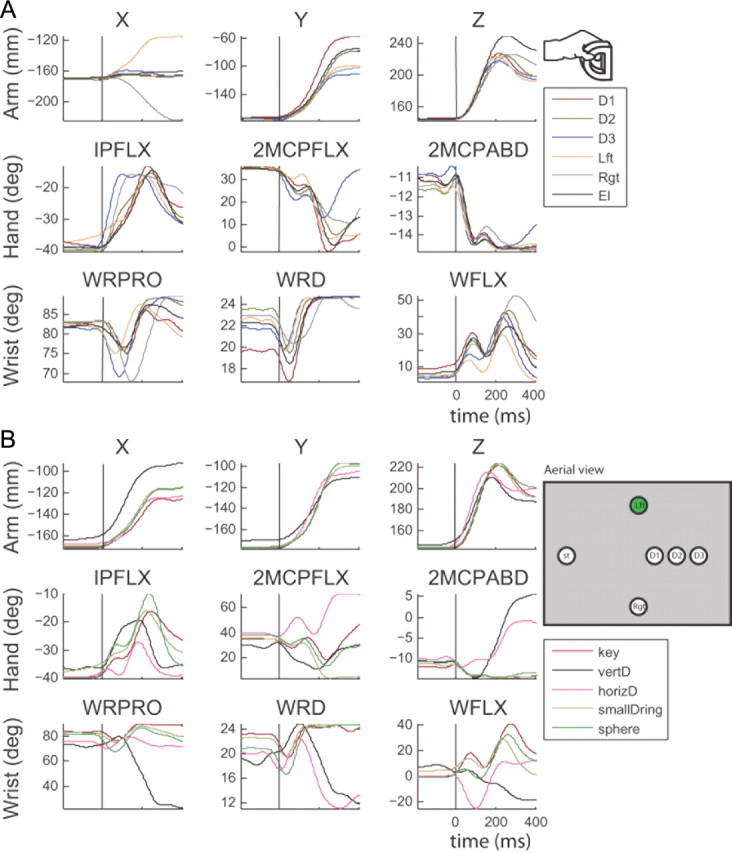
Kinematic traces for nine different features of the arm, hand, and wrist. A, Trajectories collected for reaches to 6 different locations for the small D-ring object. D1 was 12 cm away from the starting position, D2 was 10 cm away from the starting position and D3 was 8 cm away from the starting position. Lft and Rgt represent left and right targets; azimuthal angle between center and side targets was ∼35°. El represents an elevated target—10 cm from the start position, 0° in azimuth, and ∼45° in elevation. Row 1, X, Y, and Z locations of the hand. Row 2, Flexion/extension at 1PIP (IPFLX), flexion/extension of the 2MCP, and abduction/adduction of 2ABD. B, Trajectories for the reach to the left target for all objects: key (red), vertical D-ring (vertD; black), horizontal D-ring (horizD; pink), small D-Ring (yellow), sphere (green).

Results

Two datasets with a minimum of 15 trials for each combination of the five objects and seven positions were collected from each monkey (monkeys O and A). The two experiments in monkey O yielded 33 of 37 and 39 of 44 task-related units, respectively. The two experiments in monkey A yielded 32 of 50 and 39 of 82 task-related units, respectively.

In the population of units, we found examples of neurons that modulated their firing rate with respect to a given location or object. However, a neuron's selectivity for a given location was not always consistent across objects. Figure 2A shows an example of a unit that increases its firing rate when the monkey reached to the right for the vertical D-ring and the small D-ring but lost its direction selectivity when reaching for the sphere. Similarly, a neuron's selectivity for a given object was not always consistent across locations. Figure 2B shows an example of a unit that showed a preference for the sphere but only when the monkey reached to her right or in the center, not to the left. The fact that neurons show inconsistent tuning properties across objects and locations suggests that M1 neurons are not always uniquely tuned to direction or to object type. Rather, we postulate that they are tuned to a combination of proximal and distal kinematic features of the forelimb.

Figure 2.

Spike trains across trials, categorized by object and location conditions. A, Breakdown of direction selectivity across object conditions. In this example neuron, spike trains are shown across trials, aligned on the start of movement, for the left, right, and center locations (left to right), and for reaches to the vertical D-ring, sphere, and small D-ring object (top-down). The last column displays the mean firing rates and SEs across the location conditions. When the monkey reached for the vertical D-ring or the small D-ring, the neuron discharged for reaches to the right only. For reaches to the sphere, the neuron also discharged for reaches to the center target. B, Breakdown of object selectivity across locations. In this other example neuron, spike trains are displayed across trials, aligned on the start of movement, for the vertical D-ring (vertD), sphere, and horizontal D-ring (horizD) (left to right), and for the left, center, and right locations (top-down). The last column displays the mean firing rates and SEs across the object conditions. In the left direction, this example neuron does not preferentially fire for reaches to the sphere object.

We varied the types of objects and their locations to model large differences in kinematic trajectories across conditions. Examples of mean traces of the arm-, hand-, and wrist-related kinematic parameters are given for the small D-ring, across six locations in Figure 3A. Varying the object location elicits changes in the kinematic trajectories related not only to the arm, but also to the wrist and hand. Figure 3B exhibits the mean traces of the arm-, hand-, and wrist-related kinematics for the left location, across the five tested objects. Varying the object type elicits changes in the kinematic trajectories related to not only the hand, but also the arm and wrist. These observations suggest that the arm, wrist, and hand kinematics interact and covary so as to yield different joint trajectories for different combinations of objects and locations.

We developed an encoding model to predict the spiking responses of individual MI neurons based on the kinematic trajectories of the arm, wrist, and finger joints as well as the spike history of the neuron measured on multiple time scales. We used a generalized linear modeling framework where the neuron's firing rate was estimated as a function of these extrinsic and intrinsic covariates (i.e., the joint kinematics and the neuron's firing history) (see Materials and Methods for more details). A generalized linear model is a more general version of standard multiple linear regression that is suited to predict discrete integer responses (i.e., numbers of spikes emitted in a time bin) that are not normally distributed as assumed by standard regression but rather are Poisson distributed. On each trial, spike trains were simultaneously recorded from a population of neurons (Fig. 4A), while the monkey performed a reach-to-grasp behavior. To build the encoding model for each neuron, sliding windows of joint angular positions and velocities (i.e., kinematic trajectories) were associated with each 4 ms sample of the spike train whether or not a spike actually occurred or not (Fig. 4B). Unless otherwise noted, the full encoding model was used, which also included spike history terms as shown in Equation 5.

Figure 4.

Kinematic inputs to the generalized linear model. Spike trains and kinematic data for one trial. A, Spike trains from all neurons simultaneously recorded in one trial. The spikes were counted in 4 ms bins such that they yielded binary samples. For each 4 ms bin (either a 1 or a 0), we extracted a 364 ms window of all the 40 kinematic features. The gray boxes provide two examples of the windows. B, The 40 kinematic features for a given trial in normalized units.

Trajectory analysis

We used this encoding model to test whether neurons encode temporally extensive kinematic trajectories, instead of kinematic parameters at just their optimal lag from the spiking activity. First, we calculated the optimal lags between each feature and neuron's response using standard cross-correlation methods (see Material and Methods). All neurons exhibited significant cross-correlation peaks for at least 35 of the 40 kinematic features. In monkey O, a plurality of neurons exhibited an optimal lag at 100 ms across all features—where spikes precede movement by 100 ms (Fig. 5A, left panels). In monkey A, a plurality of neurons exhibited an optimal lag at 0 ms (Fig. 5A, right panels). The goal of this analysis is to show that even though we can extract an “optimal lag” across all features and neurons, the significant lags across all features are quite spread out (Fig. 5A, bottom plots), suggesting that we should consider more than one lag time between the spiking and the kinematics in the encoding model.

Figure 5.

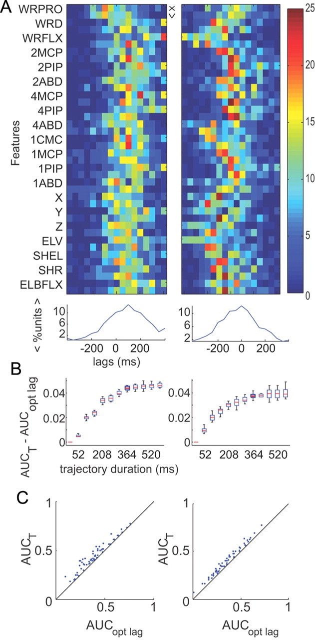
Trajectory analysis. Results across two experiments from monkey O (left) and monkey A (right). A, Optimal lag analysis. Top, Percentage of cells with significant lags across features. Colorbar represents percentage of cells. Each feature has a position (X) and velocity (V) term. Bottom, Mean percentage of cells across features as a function of lag time. Optimal lag across features for monkey O was found to be 100 ms. Optimal lag for monkey A was found to be 0 ms. B, Difference between predictive powers of trajectory model (AUC_T) and optimal lag model (AUC_{opt lag}) for an example neuron in each monkey. Using a combination of a Kruskal–Wallis test followed by pairwise Wilcoxon rank sum tests, we assessed that the predictive power attained a value that was not significantly different than its maximum at a duration of 364 ms. C, Scatter plot showing difference in predictive power between the trajectory model (364 ms in duration) and the optimal lag model (where all features were included at their optimal lag) across neurons. Each point represents a neuron.

To test whether kinematic trajectories yield significantly higher predictive power than the kinematics at their optimal lag, we tabulated the predictive power of each neuron as we increased the duration of the trajectory starting at the optimal lag for the given monkey (Fig. 5B). Trajectory duration was increased in the following three different orders: in the first case, positive and negative lags were added consecutively. In the second case, positive lags were added first, then negative lags. In the third case, negative lags were added first, then positive lags. Positive lags should be interpreted as spikes preceding movement. For each unit, we tabulated the difference in predictive power between a model that included all the kinematics at increasing durations and a model that only included the optimal lag. Figure 5B shows these differences in predictive power across cumulative increases in trajectory duration for two example neurons (monkey O on the left and monkey A on the right). The box plot shows the variability across the cross-validation folds. We found that the predictive power of the majority of the neurons (77% for monkey O and 68% for monkey A) reached a plateau for a trajectory of at least 364 ms in duration. For each neuron, the duration of the trajectory was determined by increasing its duration until the predictive power of the neuron was no longer significantly lower than the maximum achievable predictive power across all durations—the plateau (rank_Wil, p > 0.05). Using a trajectory duration of 364 ms, we tested which starting lag yielded the highest predictive power. On a population level, we found that starting the 364 ms trajectory at −44 ms yielded significantly higher predictive power than starting a trajectory of the same duration at 8, −148, or −200 ms (paired rank_Wil, p < 0.05 in all cases). However, starting the trajectory at −96 ms did not yield a significantly higher predictive power (paired rank_Wil, p = 0.07 monkey 0, p = 0.1 monkey A), suggesting that the optimal starting lag could range between −44 and −96 ms. For the remainder of the study, we opted to test 364 ms trajectories that started at −44 ms and ended at +320 ms (i.e., eight lag times). Over the population of neurons in both monkeys, the predictive power of the model with all features using a 364 ms trajectory beginning at −44 ms was significantly stronger than a model that used all features at just their optimal lags (paired rank_Wil, p < 0.05 in both monkeys; Fig. 5C).

Feature analysis

To test whether each neuron encoded reach and/or grasp components, we compared the predictive power of a model that included all features versus one where the reach or grasp features were removed. We define a neuron as encoding a category of features—reach or grasp category—if there was an associated significant drop in predictive power (paired rank_Wil, p < 0.05) when all kinematic features associated with a given category (i.e., proximal limb kinematics of the arm for the reach category and distal limb kinematics including wrist and fingers for the grasp category) were removed from the encoding model. The distributions of the reach- and grasp-related neurons were different across monkeys. In monkey O, 9%, 15%, and 72% of neurons, respectively, encoded grasp, reach, and both categories (Fig. 6A, first panel). In monkey A, 31%, 17%, and 33% of neurons, respectively, encoded grasp, reach, and both categories (Fig. 6A, third panel). Using the same paradigm, we also tested whether neurons encoded position or velocity features. Velocity and position encoding was similar across monkeys. For monkey O, 25% of neurons encoded velocity, 8% encoded position, and 56% encoded both velocity and position (Fig. 6A, second panel). For monkey A, 23% of neurons encoded velocity, 8% encoded position, and 46% encoded both position and velocity (Fig. 6A, fourth panel). We also examined the topographic organization of reach, grasp, and reach and grasp neurons across the implanted array. Across all four datasets, two in each monkey, we found a highly distributed pattern of proximal and distal representations of the limb on the precentral gyrus with no clear spatial structure (Fig. 6B).

Figure 6.

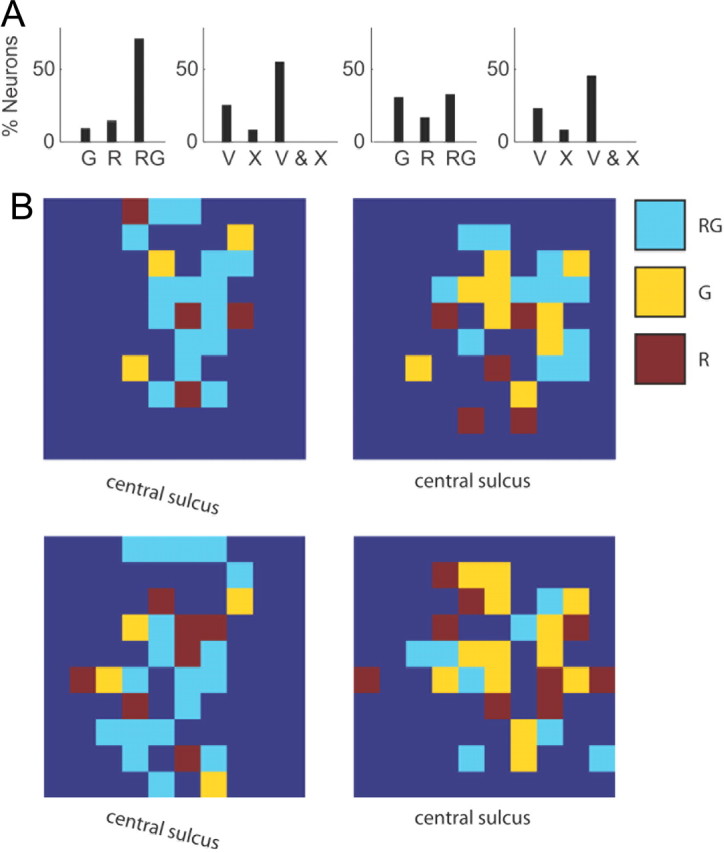
Summary of tuning properties of neurons. A, Left, Bar graph plot the percentage of neurons that are tuned to grasp (G), reach (R), and both reach and grasp (RG) for monkey O. Left middle, Bar graph plot the percentage of neurons that are velocity-tuned (V), position-tuned (X), and velocity and position-tuned for monkey O. Middle right and right, Same as first two panels but for monkey A. B, Spatial locations of neurons tuned to grasp (yellow), reach (red), and reach and grasp (light blue) on the electrode array for two different datasets in monkey O (left) and monkey A (right).

Though most features increased the predictive power of the neurons, some features yielded a more significant increase in predictive power. To test which features were most significant for each neuron, we compared the predictive power of a set of encoding models built with each feature trajectory separately. Figure 7A displays the difference in predictive power between each feature and the mean predictive power across single features. The features are broken down into reach-related (top panels) and grasp-related (bottom panels) features. On a population level, the reach-related features tended be more significant than the grasp-related features (monkey O: rank_Wil, p < 0.001; monkey A: rank_Wil, p < 0.001). For both reach- and grasp-related features, the velocity terms tended to be more significant than the position terms (monkey O: paired rank_Wil, p < 0.001, monkey A: paired rank_Wil, p < 0.001). Among the reach-related features, Y and Z Cartesian velocity of the hand were the most significant features (KW_A test, followed by pairwise rank_Wil, p < 0.05). Among the grasp-related features, flexion/extension velocities at the metacarpo-phalangeal joints of the index and ring finger and pronation/supination velocity of the wrist were the most significant features (KW_A, followed by pairwise rank_Wil, p < 0.05). Finally, we tested whether there was a significant increase in predictive power when the model included all feature trajectories versus just the one feature trajectory that yielded the highest predictive power. For both monkeys, the model that included all features significantly increased the predictive power of neurons (Fig. 7B, pairwise rank_Wil, p < 0.001 for O on the left; pairwise rank_Wil, p = 0.0015 for A on the right).

Figure 7.

Reach and grasp-related cells in MI in two monkeys; subject O (left) and subject A (right). A, Difference in predictive power between a model that only included the feature denoted on the y-axis and the mean predictive power across all single features. Colors represent the predictive power of a model with a given feature subtracted by the mean predictive power across all single features (AUC − < AUC >). Top, Includes neurons that encoded reach features and reach and grasp-related features. Bottom, Includes neurons that encoded grasp-related and reach and grasp-related features. Each column corresponds to a single neuron. B, Comparison of predictive power between a model that included all the feature trajectories (full model) and one that only included the feature trajectory that yielded the highest predictive power for each neuron for monkey O (left) and monkey A (right). Each point represents a neuron.

Principal component analysis

Throughout our analyses, we calculated the principal components of all the external covariates to reduce the dimensionality of the kinematics. Thirty principal components accounted for 80% of the variance in the 320 dimensions of kinematics in our model (Fig. 8A). To test which PCs were most significant for each neuron, we built encoding models that included each principal component and tested which model yielded a predictive power that was significantly higher than the mean across all components (KW_A, followed by rank_Wil, p < 0.05). Figure 8B displays the increase in predictive power for each PC model, with respect to the mean predictive power across all tested models for each recorded neuron. Figure 8C shows the median and range of predictive powers across neurons for each PC model. The most significant principal components for monkey O were the first, second, and fourth principal components: 61%, 64%, and 50% of neurons displayed a significant increase in predictive power compared with the other components (KW_A test, followed by pairwise rank_Wil test, p < 0.05). For monkey A, the first and third principal components were the most significant: in both cases, 75% of neurons showed a significant increase in predictive power (KW_A test followed by pairwise rank_Wil test, p < 0.05).

Figure 8.

Principal component analysis. A, Percentage of variance accounted for by principal components for all four experiments. A mean of 30 PCs were required to account for 80% of the variance. Monkey O's experiments are displayed in red and orange, and monkey A's experiments are displayed in the two shades of blue. B, Difference between predictive power for a given principal component and the mean predictive power across all 30 single principal components. Top plot displays results for monkey O, and bottom plot displays results for monkey A. Grayscale map represents difference in predictive power. The y-axis shows values across cells. C, Box plots of the median and range of differences in predictive power across neurons for the first 15 principal components for monkey O (top) and monkey A (bottom).

We also tested how many principal components were required to reach the maximum predictive power of each neuron. The increase in predictive power relative to the history model as principal components were cumulatively added to the model is shown for an example neuron from each monkey in Figure 9A. In the example neuron for monkey O, four principal components were required to reach a predictive power that was not significantly different from the full model (paired rank_Wil, p < 0.05 up to third component, p = 0.17 for the fourth component). In the example neuron for monkey A, three principal components were required to reach a predictive power that was not significantly different from the full model (paired rank_Wil, p < 0.001 up to second and p = 0.25 for the third component). Across all neurons for monkey O, a mean of five principal components was required to reach the predictive power of the full model (Fig. 9B, left), while for monkey A a mean of four principal components was required to reach the predictive power of the full model (Fig. 9B, right). The first five eigenvectors were highly similar across experiments for a given monkey and also across monkeys: the correlation coefficients between pairwise comparisons of each eigenvector across all four datasets were all significant and high (r_eig1 = 0.87 ± 0.04, r_eig2 = 0.65 ± 0.08, r_eig3 = 0.66 ± 0.08, r_eig4 = 0.60 ± 0.10, r_eig5 = 0.55 ± 0.11). Further, the correlation coefficients of the eigenvectors within monkeys were generally higher than the correlation coefficients across monkeys.

Figure 9.

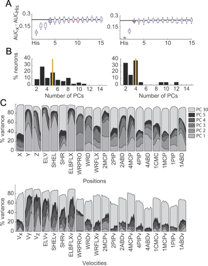
Principal component analysis for monkey O (left) and monkey A (right). A, Increase in predictive power with each added principal component for an example cell in monkey O (left) and one in monkey A (right). The predictive power of the full model is displayed by the black line. B, Number of PCs required to reach a predictive power that was not significantly different from the predictive power of the full model (30 PCs). Monkey O required a mean of five principal components, whereas monkey A required a mean of four principal components (see orange lines). C, Percentage of variance accounted for across trajectories with the cumulative addition of principal components up to 30 components (see legend) for position trajectories (top) and velocity trajectories (bottom).

We examined the first five principal components to determine which kinematic features were emphasized. To do this, we computed the percentage variance accounted for per feature, as principal components were cumulatively added. Figure 9C displays our results for the cumulative addition of five components, and the result for reconstructions using the full 30 principal components. The variability in the position trajectories was captured with fewer components than the velocity trajectories. However, some features were better captured than others (i.e., inhomogeneous capture of features), and these features were consistent across positions and velocities: the first five principal components captured more variability in ELV of the shoulder, the SHEL, flexion and extension of the elbow, wrist positions Y and Z, pronation and supination of the wrist, and the flexion and extension of the metacarpo-phalangeal joints of the index and ring fingers. For the position terms only, abduction and adduction of the thumb, index, and ring fingers and ulnar and radial deviation about the wrist were also captured by the five principal components.

Spike history

We sought to determine which spike history terms were most significant across the population of recorded neurons. To model these spiking history components, we defined a set of basis vectors (Fig. 10A). The vectors were designed to account for broader windows of time as history went further back into the past. The spike train was filtered with each of these basis vectors (Fig. 10B). The first spike history term is the original spike train convolved with B1 from Figure 10A: it represents spiking history immediately preceding the present and is filtered over a narrow time window, compared with the last spike history term, filtered over a very large time window, B7.

To find the significant spike history terms, we first calculated the coefficients using training data that were sampled during the premovement period. We then calculated the predictions using the data sampled during the entire trial duration. A model was built using the kinematic covariates and each of the single spike history terms. A spike history term was considered to be significant if its predictive power was significantly larger than at least one of the other spike history terms (KW_A, followed by rank_Wil, p < 0.05). The difference in predictive power of each model and the mean predictive power across all single spike history terms was calculated for each neuron separately in monkey O (Fig. 10C, left) and monkey A (Fig. 10C, right). We found that for monkey O, the first and second spike history terms, at respective basis centers of 8 and 12 ms, were more significant than the other terms (pairwise comparisons, rank_Wil, p_term1 < 0.001 in all cases, and p_term2 < 0.001 for all terms except term 1 since predictive powers tended to be larger than those for term 2). For monkey A, only the second term was found to be more significant than the spike history term at a basis center of 60 ms (rank_Wil, p < 0.001).

We also compared the predictive power of a model that only included the kinematic covariates to one that only included the spike history covariates. Because of their slow temporal frequency, the kinematics are designed to capture slower fluctuations in firing rate, whereas spike history is designed to model faster fluctuations in rate due to refractoriness, bursting, and oscillations (Fig. 11A). Notice the middle panel in Figure 11A shows “blurred” versions of the original spike trains because the slowly varying kinematics did not model the fast changes in spiking activity. On the other hand, there were many examples where the slow fluctuations were well modeled by the kinematics, whereas the faster fluctuations were not well captured by spike history (Fig. 11B). In fact, we found that the kinematic model yielded significantly higher predictive power than the spike history model on a population level for both animals (paired rank_Wil, p < 0.001 for both monkeys) (Fig. 11C).

Figure 11.

Predictive power of spike history versus kinematics. A, Actual spikes for 50 randomly selected trials of a neuron that yielded significantly higher predictive power for the spike history model—see green circle in C (left). Spike predictions of the kinematics model (middle) and predictions of the spike history model (right). B, same as A but for a neuron that yielded higher predictive power for the kinematics model—see red circle in C. C, Predictive power of an encoding model with kinematic covariates compared with the predictive power of an encoding model with spike history covariates for monkey O (left) and monkey A (right). Each point in the scatter plot is a neuron.

Although generally not capable of capturing fine temporal modulations in rate, the kinematics could more precisely predict the onset time of the slow but large movement-related modulation. Onset times were calculated by finding the lag at which there was a significant peak in the cross-correlation between the actual spikes and the predictions of the kinematic and spike history models. The kinematic model yielded significant peaks in the cross-correlations that were closer to a lag of 0 ms, compared with the spike history model. In monkey O, the median lag was 4 ms for the kinematic model and 16 ms for the spike history model; in monkey A, the median lag was 8 ms for the kinematics model and 28 ms for the spike history model. In both cases, the predictions of the history model lagged behind the predictions of the kinematic model. These results suggest that the kinematic model more precisely predicts the onset of spike rate modulation.

Generalization

To test whether the encoding model is context dependent, we built the model on training data collected from four of the five objects and tested its predictive power on data from the fifth object. The five resulting models are called “restricted” models. The actual spike trains for leftward reaches toward the five objects are given for an example neuron in Figure 12A. The predicted spike counts for the full model and the restricted model are then given in Figure 12, B and C, respectively. The predictive power of the restricted models across all neurons was well above chance (rank_Wil against a median of 0.5, p < 0.001 in all cases) indicating that all the models generalized to a certain extent. To compare the performance of the restricted models to the full model, we used a Kruskal–Wallis ANOVA test followed by pairwise Wilcoxon rank sum tests (Fig. 12D). We found that the full model was not significantly different than any of the restricted models, except for the restricted model that omitted the vertical D-ring in monkey O (monkey O: p_key = 0.85, p_VertD = 0.01, p_HorizD = 0.0742, p_smallD = 0.90, p_sphere = 0.99; monkey A: p_key = 0.06, p_VertD = 0.39, p_HorizD = 0.07, p_smallD = 0.80, p_sphere = 0.48).

Figure 12.

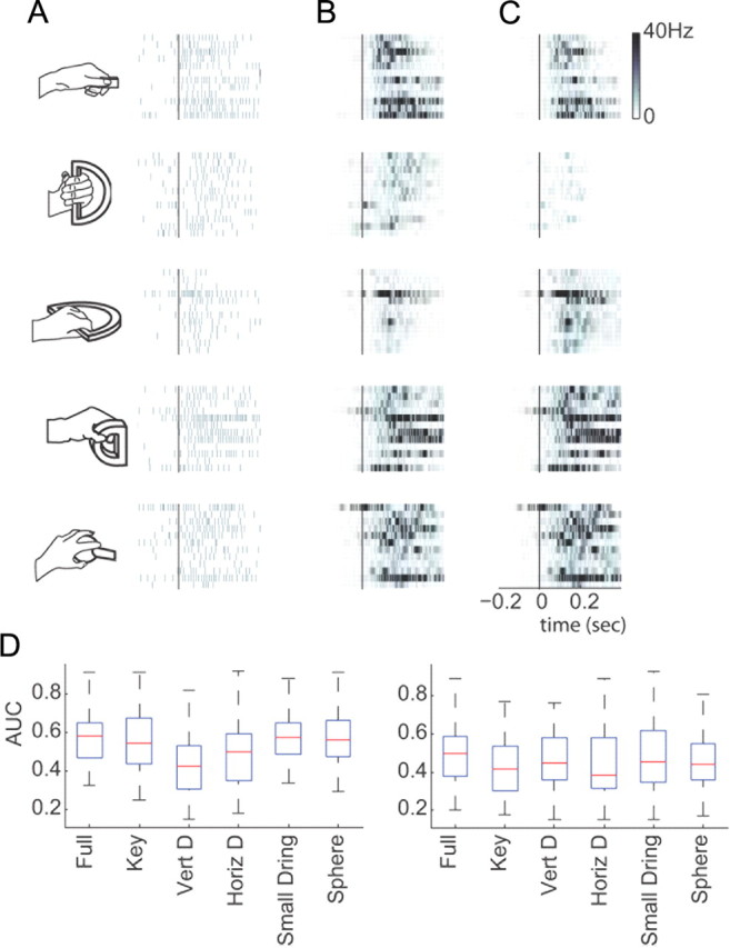
Testing for model generalization. A, Example neuron's spike trains across trials while monkey reached for objects (illustrated to the left) positioned in one location (from monkey O). Trials are aligned on movement onset. B, Predicted firing rate using a model that was built with all the training data. C, Predicted firing rate using a model that was built using only data from the other four objects (omitted object, from top to bottom row, is represented by the illustration at the left and corresponds to the key grip, the vertical D-ring (Vert D), the horizontal D-ring (Horiz D), the small D-ring and the sphere. D, Box plots showing median and range of predictive power for full and restricted models for monkey O (left) and monkey A (right) across the two experiments. The median predictive power for monkey O was 0.58, while the median predictive power for monkey A was 0.50.

Discussion

Individual MI neurons control movement by forming synergies that involve both proximal and distal musculature of the upper limb (Shinoda et al., 1981; McKiernan et al., 1998). Furthermore, their firing activity has been shown to correlate to kinematics that represent both reach and grasp (Stark et al., 2007; Vargas-Irwin et al., 2010). This study extends these findings by modeling the time-varying interactions between reach and grasp kinematics. To reduce the dimensionality of the movement, we took the principal components of the 320 kinematic parameters. Though 30 principal components accounted for 80% of the movement variability, our encoding model of single-neuron activity reached a plateau with just five components. These results suggest that MI neurons on the precentral gyrus encode the more general aspects of a reach-to-grasp movement, rather than the finer adjustments in movement that would be captured by the higher principal components. Our results also suggest that MI neurons may have adapted to encode natural coordination patterns that emerge during reach-to-grasp movements instead of movements about single joints.

Trajectory encoding

Our results show that neurons encode multiple reach and grasp features as temporally extended trajectories, rather than static movement parameters. That is, MI neurons encode a reach-to-grasp movement by means of time-varying trajectories of ∼350 ms in duration that represent the coordination of the arm and hand rather than single joint angle kinematics at one lag with respect to spiking. By modeling the kinematics as joint trajectories instead of static movement parameters, we were able to characterize how MI neurons encode the time-dependent covariance between the kinematic features. We have previously tested trajectory-based encoding models on constrained and isolated grasping and reaching behaviors (Hatsopoulos et al., 2007, 2010; Saleh et al., 2010). A similar trajectory-based approach has been applied to muscle activity instead of cortical activity during constrained human arm movements (Pruszynski et al., 2010). We now extend these findings by examining a more ethologically relevant and unconstrained movement, where reaching and grasping are examined as a single coordinated movement (Hatsopoulos et al., 2010).

Our findings that the discharge of motor cortical neurons is captured by a movement trajectory of such long duration may seem at first glance counterintuitive. However, two experimental observations should be noted. First, the fact that the trajectory extends back in time before the occurrence of a spike is consistent with data demonstrating that motor cortical neurons exhibit somatosensory responses during passive movement (Fetz and Cheney, 1980; Suminski et al., 2009). Therefore, the negative time lags in the encoded trajectory may represent sensory effects on motor cortical discharge. Second, the extended duration of the trajectory following the spike could be explained by persistent inward currents that have been shown to generate plateau potentials in motor neurons in the spinal cord that extend for long periods of time even after inputs to the neurons are terminated (Lee and Heckman, 1998; Heckman et al., 2003).

Feature encoding

Multiple psychophysics studies have described the spatiotemporal dependencies between the kinematics that describe reach-to-grasp behavior, focusing on hand transport and grasp aperture measured between the thumb and index finger (Jeannerod, 1984; Jakobson and Goodale, 1991; Paulignan et al., 1991a,b, 1997; Haggard and Wing, 1998). This study extends the number of features that represent hand shape (i.e., 26 grasp features) and transport (i.e., 14 reach features) during a prehensile movement and examines whether MI neurons encode these joint trajectories. We show that the precentral gyrus is intermingled with neurons that encode reach-related features, grasp-related features, or both. Intracortical microelectrode stimulation studies have indicated that the motor cortex has a somatotopic organization in which a central core primarily within the central sulcus represents distal hand movements surrounded by a proximal arm area shaped like a horseshoe extending onto the precentral gyrus (Kwan et al., 1978a; Park et al., 2001). Between these two areas, an intermediate zone is populated with a preponderance of neurons that project to both distal and proximal arm musculature. Given that we encountered a plurality of neurons that encoded both reach- and grasp-related kinematics, these results suggest that our electrode arrays targeted this intermediate zone.

Among the grasp features, pronation and supination of the wrist, along with flexion and extension of the metacarpo-phalangeal joints of the index and ring fingers, accounted for more of the variance in spike rate modulation than other features. Interestingly, we did not see a strong neural representation of thumb movements. This may partially be due to the fact that monkeys, compared with humans, have a shorter thumb relative to the length of the other fingers and make less use of it in the prehensile movements we tested (Marzke, 1994). It may also indicate that the microelectrodes were not ideally placed to record from thumb movement-related neurons. In terms of the reach features, abduction/adduction and flexion/extension of the shoulder, flexion and extension of the elbow, and hand velocity in the Y and Z directions accounted for more of the variance in spike rate modulation than the other features.

Spike history

Though all spike history terms were significant for the majority of neurons, the first and second terms, representing faster changes in firing activity, on the order of 8–12 ms, tended to yield larger increases in predictive power. The third to seventh terms represent slower changes in a neuron's spiking history and may provide information that is redundant with the kinematics, which occur on a similar time scale. We also show that a model built with the kinematic trajectories alone consistently performed better than a model built with just the spike history terms. This result is somewhat inconsistent with those of our previous article, which showed that a significant number of MI neurons yielded spike history models that performed better than the kinematic models for an isolated grasping behavior (Saleh et al., 2010). There are two reasons that likely explain this discrepancy. First, since the array was placed in an area that represents both arm- and hand-related parameters, it is possible that some of the neuronal variability unaccounted for during isolated grasping could be accounted for during reach-to-grasp movements, thus resulting in consistently stronger predictive power from reach and grasp kinematics relative to spike history. Second, unlike our previous study, the coefficients of the spike history terms were built from data extracted during the premovement period. We did this on purpose to characterize the intrinsic neural dynamics that are not confounded with movement-related activity. In our previous study, the spike history terms could be capturing movement-related activity and, thus, unfairly inflating the predictive power of spike history.

Prediction results

The median predictive power that could be achieved with our encoding model was 0.58 in monkey O and 0.5 in monkey A, consistent with the results we report for a similar model, evaluated for an isolated grasping task (Saleh et al., 2010). It is important to note that in the previous study, the predictive power was taken to be the AUC, which takes a value between 0.5 and 1. In the current study, the predictive power was calculated as 2 * AUC − 1, so that it could take on values between 0 and 1. The variability in predictive power across neurons was quite large, with values ranging between 0.22 and 0.89. This variability suggests that neurons encode the tested intrinsic and extrinsic covariates to various extents. Neurons with lower predictive power may be involved in other cortical functions that are not represented by the tested covariates.

Intermonkey differences

There were some interesting differences in our results between the two monkeys. First, monkey A had significantly more neurons that were tuned to grasp kinematics than did monkey O. This may be explained by the fact that monkey A's array was placed slightly more lateral and closer to the sulcus than monkey O's array (Fig. 1D). According to several studies, distal representations of the hand tend to be located closer to the central sulcus and lateral to the proximal representations of the arm (Kwan et al., 1978b; Strick and Preston, 1978; He et al., 1993; Park et al., 2001). The somatotopy of MI would dictate that an array that is placed closer to the center sulcus and more lateral, like monkey A's array, would record more neurons that are tuned to distal features, so that monkey A's higher density of grasp-related neurons are compatible with this finding. Second, although most restricted models built on a subset of objects generalized quite well, the restricted model that was tested on the data from the vertical D-ring object in monkey O did not perform as well as the other restricted models. This may be explained by a difference in movement strategies between the two monkeys. The vertical D-ring elicited considerably more supination about the wrist than any other object for monkey O, unlike monkey A.

Concluding remarks

By showing that MI neurons encode spatiotemporal patterns of kinematics of the arm and hand that can be described by as little as five principal components, our results support Bernstein's classic notion that the cortex simplifies the control of multiple degrees of freedom by coupling output variables at the kinematic level (Bernstein, 1967). Though we show that using these kinematic synergies yields robust predictions of single neuron responses tied to reach-to-grasp behaviors to different locations and objects, it remains to be examined how these same synergies—and the neurons that encode them—contribute to other upper limb behaviors (Tresch and Jarc, 2009). Future studies might investigate how MI neurons control other ethologically relevant movements like climbing or feeding (Macfarlane and Graziano, 2009). It also remains to be tested how populations of neurons work together to encode ethologically relevant movements along with finer adjustments, such as those observed in response to perturbations of a planned movement (Paulignan et al., 1991a,b; Haggard and Wing, 1995).

References

- Bernstein N. The coordination and regulation of movements. London: Pergamon; 1967. [Google Scholar]
- Chen D, Fetz EE. Characteristic membrane potential trajectories in primate sensorimotor cortex neurons recorded in vivo. J Neurophysiol. 2005;94:2713–2725. doi: 10.1152/jn.00024.2005. [DOI] [PubMed] [Google Scholar]
- Donoghue JP, Leibovic S, Sanes JN. Organization of the forelimb area in squirrel monkey motor cortex: representation of digit, wrist, and elbow muscles. Exp Brain Res. 1992;89:1–19. doi: 10.1007/BF00228996. [DOI] [PubMed] [Google Scholar]
- Fawcett T. An introduction to ROC analysis. Pattern Recognit Lett. 2006;27:861–874. [Google Scholar]
- Fetz EE, Cheney PD. Postspike facilitation of forelimb muscle activity by primate corticomotoneuronal cells. J Neurophysiol. 1980;44:751–772. doi: 10.1152/jn.1980.44.4.751. [DOI] [PubMed] [Google Scholar]
- Haggard P, Wing A. Coordinated responses following mechanical perturbation of the arm during prehension. Exp Brain Res. 1995;102:483–494. doi: 10.1007/BF00230652. [DOI] [PubMed] [Google Scholar]
- Haggard P, Wing A. Coordination of hand aperture with the spatial path of hand transport. Exp Brain Res. 1998;118:286–292. doi: 10.1007/s002210050283. [DOI] [PubMed] [Google Scholar]
- Hatsopoulos NG, Xu Q, Amit Y. Encoding of movement fragments in the motor cortex. J Neurosci. 2007;27:5105–5114. doi: 10.1523/JNEUROSCI.3570-06.2007. [DOI] [PMC free article] [PubMed] [Google Scholar]
- Hatsopoulos N, Saleh M, Mattiello JA. Encoding and beyond in the motor cortex. In: Platt ML, Ghazanfar AA, editors. Primate neuroethology. New York: Oxford UP; 2010. pp. 256–272. [Google Scholar]
- He SQ, Dum RP, Strick PL. Topographic organization of corticospinal projections from the frontal lobe: motor areas on the lateral surface of the hemisphere. J Neurosci. 1993;13:952–980. doi: 10.1523/JNEUROSCI.13-03-00952.1993. [DOI] [PMC free article] [PubMed] [Google Scholar]
- Heckman CJ, Lee RH, Brownstone RM. Hyperexcitable dendrites in motoneurons and their neuromodulatory control during motor behavior. Trends Neurosci. 2003;26:688–695. doi: 10.1016/j.tins.2003.10.002. [DOI] [PubMed] [Google Scholar]
- Hille B. Ion channels of excitable membranes. Sunderland, MA: Sinauer Associates; 2001. [Google Scholar]
- Hocherman S, Wise SP. Effects of hand movement path on motor cortical activity in awake, behaving rhesus monkeys. Exp Brain Res. 1991;83:285–302. doi: 10.1007/BF00231153. [DOI] [PubMed] [Google Scholar]
- Holzbaur KR, Murray WM, Delp SL. A model of the upper extremity for simulating musculoskeletal surgery and analyzing neuromuscular control. Ann Biomed Eng. 2005;33:829–840. doi: 10.1007/s10439-005-3320-7. [DOI] [PubMed] [Google Scholar]
- Jakobson LS, Goodale MA. Factors affecting higher-order movement planning: a kinematic analysis of human prehension. Exp Brain Res. 1991;86:199–208. doi: 10.1007/BF00231054. [DOI] [PubMed] [Google Scholar]
- Jeannerod M. The timing of natural prehension movements. J Mot Behav. 1984;16:235–254. doi: 10.1080/00222895.1984.10735319. [DOI] [PubMed] [Google Scholar]
- Keat J, Reinagel P, Reid RC, Meister M. Predicting every spike: a model for the responses of visual neurons. Neuron. 2001;30:803–817. doi: 10.1016/s0896-6273(01)00322-1. [DOI] [PubMed] [Google Scholar]
- Kwan HC, MacKay WA, Murphy JT, Wong YC. Spatial organization of precentral cortex in awake primates. II. Motor outputs. J Neurophysiol. 1978a;41:1120–1131. doi: 10.1152/jn.1978.41.5.1120. [DOI] [PubMed] [Google Scholar]
- Kwan HC, Mackay WA, Murphy JT, Wong YC. An intracortical microstimulation study of output organization in precentral cortex of awake primates. J Physiol (Paris) 1978b;74:231–233. [PubMed] [Google Scholar]
- Lee RH, Heckman CJ. Bistability in spinal motorneurons in vivo: systematic variations in persistent inward current. J Neurophysiol. 1998;80:583–593. doi: 10.1152/jn.1998.80.2.583. [DOI] [PubMed] [Google Scholar]
- Macfarlane NB, Graziano MS. Diversity of grip in macaca mulatta. Exp Brain Res. 2009;197:255–268. doi: 10.1007/s00221-009-1909-z. [DOI] [PubMed] [Google Scholar]
- Marzke M. Evolution. In: Bennett KMB CU, editor. Insights into the reach to grasp movement. Amsterdam: Elsevier; 1994. pp. 19–35. [Google Scholar]
- Mason CR, Gomez JE, Ebner TJ. Hand synergies during reach-to-grasp. J Neurophysiol. 2001;86:2896–2910. doi: 10.1152/jn.2001.86.6.2896. [DOI] [PubMed] [Google Scholar]
- Maynard EM, Nordhausen CT, Normann RA. The Utah intracortical electrode array: a recording structure for potential brain-computer interfaces. Electroencephalogr Clin Neurophysiol. 1997;102:228–239. doi: 10.1016/s0013-4694(96)95176-0. [DOI] [PubMed] [Google Scholar]
- Maynard EM, Hatsopoulos NG, Ojakangas CL, Acuna BD, Sanes JN, Normann RA, Donoghue JP. Neuronal interactions improve cortical population coding of movement direction. J Neurosci. 1999;19:8083–8093. doi: 10.1523/JNEUROSCI.19-18-08083.1999. [DOI] [PMC free article] [PubMed] [Google Scholar]
- McKiernan BJ, Marcario JK, Karrer JH, Cheney PD. Corticomotoneuronal postspike effects in shoulder, elbow, wrist, digit, and intrinsic hand muscles during a reach and prehension task. J Neurophysiol. 1998;80:1961–1980. doi: 10.1152/jn.1998.80.4.1961. [DOI] [PubMed] [Google Scholar]
- Paninski L, Pillow JW, Simoncelli EP. Maximum likelihood estimation of a stochastic integrate-and-fire neural encoding model. Neural Comput. 2004;16:2533–2561. doi: 10.1162/0899766042321797. [DOI] [PubMed] [Google Scholar]
- Park MC, Belhaj-Saïf A, Gordon M, Cheney PD. Consistent features in the forelimb representation of primary motor cortex in rhesus macaques. J Neurosci. 2001;21:2784–2792. doi: 10.1523/JNEUROSCI.21-08-02784.2001. [DOI] [PMC free article] [PubMed] [Google Scholar]
- Paulignan Y, MacKenzie C, Marteniuk R, Jeannerod M. Selective perturbation of visual input during prehension movements. 1. The effects of changing object position. Exp Brain Res. 1991a;83:502–512. doi: 10.1007/BF00229827. [DOI] [PubMed] [Google Scholar]
- Paulignan Y, Jeannerod M, MacKenzie C, Marteniuk R. Selective perturbation of visual input during prehension movements. 2. The effects of changing object size. Exp Brain Res. 1991b;87:407–420. doi: 10.1007/BF00231858. [DOI] [PubMed] [Google Scholar]
- Paulignan Y, Frak VG, Toni I, Jeannerod M. Influence of object position and size on human prehension movements. Exp Brain Res. 1997;114:226–234. doi: 10.1007/pl00005631. [DOI] [PubMed] [Google Scholar]
- Pillow JW, Shlens J, Paninski L, Sher A, Litke AM, Chichilnisky EJ, Simoncelli EP. Spatio-temporal correlations and visual signalling in a complete neuronal population. Nature. 2008;454:995–999. doi: 10.1038/nature07140. [DOI] [PMC free article] [PubMed] [Google Scholar]
- Pruszynski JA, Lillicrap TP, Scott SH. Complex spatiotemporal tuning in human upper-limb muscles. J Neurophysiol. 2010;103:564–572. doi: 10.1152/jn.00791.2009. [DOI] [PubMed] [Google Scholar]
- Rousche PJ, Normann RA. A method for pneumatically inserting an array of penetrating electrodes into cortical tissue. Ann Biomed Eng. 1992;20:413–422. doi: 10.1007/BF02368133. [DOI] [PubMed] [Google Scholar]
- Saleh M, Takahashi K, Amit Y, Hatsopoulos NG. Encoding of coordinated grasp trajectories in primary motor cortex. J Neurosci. 2010;30:17079–17090. doi: 10.1523/JNEUROSCI.2558-10.2010. [DOI] [PMC free article] [PubMed] [Google Scholar]
- Santello M, Soechting JF. Gradual molding of the hand to object contours. J Neurophysiol. 1998;79:1307–1320. doi: 10.1152/jn.1998.79.3.1307. [DOI] [PubMed] [Google Scholar]
- Santello M, Flanders M, Soechting JF. Postural hand synergies for tool use. J Neurosci. 1998;18:10105–10115. doi: 10.1523/JNEUROSCI.18-23-10105.1998. [DOI] [PMC free article] [PubMed] [Google Scholar]
- Santello M, Flanders M, Soechting JF. Patterns of hand motion during grasping and the influence of sensory guidance. J Neurosci. 2002;22:1426–1435. doi: 10.1523/JNEUROSCI.22-04-01426.2002. [DOI] [PMC free article] [PubMed] [Google Scholar]
- Shinoda Y, Yokota J, Futami T. Divergent projection of individual corticospinal axons to motoneurons of multiple muscles in the monkey. Neurosci Lett. 1981;23:7–12. doi: 10.1016/0304-3940(81)90182-8. [DOI] [PubMed] [Google Scholar]
- Stark E, Drori R, Asher I, Ben-Shaul Y, Abeles M. Distinct movement parameters are represented by different neurons in the motor cortex. Eur J Neurosci. 2007;26:1055–1066. doi: 10.1111/j.1460-9568.2007.05711.x. [DOI] [PubMed] [Google Scholar]
- Strick PL, Preston JB. Multiple representation in the primate motor cortex. Brain Res. 1978;154:366–370. doi: 10.1016/0006-8993(78)90707-2. [DOI] [PubMed] [Google Scholar]
- Suminski AJ, Tkach DC, Hatsopoulos NG. Exploiting multiple sensory modalities in brain-machine interfaces. Neural Netw. 2009;22:1224–1234. doi: 10.1016/j.neunet.2009.05.006. [DOI] [PMC free article] [PubMed] [Google Scholar]
- Tresch MC, Jarc A. The case for and against muscle synergies. Curr Opin Neurobiol. 2009;19:601–607. doi: 10.1016/j.conb.2009.09.002. [DOI] [PMC free article] [PubMed] [Google Scholar]
- Truccolo W, Eden UT, Fellows MR, Donoghue JP, Brown EN. A point process framework for relating neural spiking activity to spiking history, neural ensemble, and extrinsic covariate effects. J Neurophysiol. 2005;93:1074–1089. doi: 10.1152/jn.00697.2004. [DOI] [PubMed] [Google Scholar]
- Truccolo W, Friehs GM, Donoghue JP, Hochberg LR. Primary motor cortex tuning to intended movement kinematics in humans with tetraplegia. J Neurosci. 2008;28:1163–1178. doi: 10.1523/JNEUROSCI.4415-07.2008. [DOI] [PMC free article] [PubMed] [Google Scholar]
- Truccolo W, Hochberg LR, Donoghue JP. Collective dynamics in human and monkey sensorimotor cortex: predicting single neuron spikes. Nat Neurosci. 2010;13:105–111. doi: 10.1038/nn.2455. [DOI] [PMC free article] [PubMed] [Google Scholar]
- Vargas-Irwin C, Donoghue JP. Automated spike sorting using density grid contour clustering and subtractive waveform decomposition. J Neurosci Methods. 2007;164:1–18. doi: 10.1016/j.jneumeth.2007.03.025. [DOI] [PMC free article] [PubMed] [Google Scholar]
- Vargas-Irwin CE, Shakhnarovich G, Yadollahpour P, Mislow JM, Black MJ, Donoghue JP. Decoding complete reach and grasp actions from local primary motor cortex populations. J Neurosci. 2010;30:9659–9669. doi: 10.1523/JNEUROSCI.5443-09.2010. [DOI] [PMC free article] [PubMed] [Google Scholar]