

Abstract
In any sensory system, the primary afferents constitute the first level of sensory representation and fundamentally constrain all subsequent information processing. Here, we show that the spike timing, reliability, and stimulus selectivity of primary afferents in the whisker system can be accurately described by a simple model consisting of linear stimulus filtering combined with spike feedback. We fitted the parameters of the model by recording the responses of primary afferents to filtered, white noise whisker motion in anesthetized rats. The model accurately predicted not only the response of primary afferents to white noise whisker motion (median correlation coefficient 0.92) but also to naturalistic, texture-induced whisker motion. The model accounted both for submillisecond spike-timing precision and for non-Poisson spike train structure. We found substantial diversity in the responses of the afferent population, but this diversity was accurately captured by the model: a 2D filter subspace, corresponding to different mixtures of position and velocity sensitivity, captured 94% of the variance in the stimulus selectivity. Our results suggest that the first stage of the whisker system can be well approximated as a bank of linear filters, forming an overcomplete representation of a low-dimensional feature space.
Introduction
At the first stage of any sensory system, modality-specific receptors transduce sensory stimuli into temporal patterns of action potentials. Primary afferents convey these action potentials to subsequent stations of the sensory pathway. The manner in which primary afferents encode sensory information thus fundamentally constrains all subsequent information processing. How well do we understand how primary afferents in any given sensory system encode sensory stimuli? A useful test is to formulate knowledge of the afferent's behavior as a quantitative model and to attempt to predict the afferent's response to sensory signals. A successful model will accurately capture key aspects of the neuronal response: spike timing, response reliability, spike pattern statistics, and stimulus selectivity.
Rodents use their whiskers (mystacial vibrissae) to explore the environment by means of exploratory, forward, and backward “whisking” movements. Both whisking itself and whisker-object contact evoke spikes in the primary afferents (Szwed et al., 2003; Arabzadeh et al., 2005; Leiser and Moxon, 2007; Khatri et al., 2009). The encoding mechanism is likely to involve stresses and strains within the tissues of the follicle–sinus complex (FSC), which are transduced by diverse mechanoreceptors (Mitchinson et al., 2008; Lottem and Azouz, 2011; Ebara et al., 2002). Primary afferents, with cell bodies located in the trigeminal ganglion, innervate the whisker follicle and convey information about whisker motion, encoded as patterns of action potentials, to the cerebral cortex by means of parallel, trisynaptic pathways through the brainstem and thalamus (for review, see Diamond and Arabzadeh, 2013).
Previous investigations have determined features of whisker motion to which primary afferents respond and have found that they do so with remarkable reliability and spike-timing precision (Zucker and Welker, 1969; Gibson and Welker, 1983; Lichtenstein et al., 1990; Szwed et al., 2003; Jones et al., 2004; Arabzadeh et al., 2005; Lottem and Azouz, 2011; Storchi et al., 2012). Our aim here was to capture the relationship between whisker motion and primary afferent responses in a simple model and thereby to address the following questions. What kinetic features of whisker motion (position, velocity, etc) do primary afferents encode? How diverse are different primary afferents? Can a model capture the response to random whisker motion? Can such a model generalize to whisker motion induced by whisking textured objects? Collectively, what space of kinetic features does the afferent population encode?
To investigate these issues, we recorded extracellular responses of individual primary afferents both to deflection of the whiskers with low-pass-filtered white noise (hereafter referred to as “white noise”), and to playback of texture-induced whisker motion (Wolfe et al., 2008). We found that the spike timing, reliability, and stimulus selectivity of primary afferents in the whisker system could be accurately described by a generalized linear model (GLM), consisting of linear stimulus filtering combined with spike feedback. The model not only predicted the response of primary afferents to white noise whisker motion but also generalized to texture-induced whisker motion. Analysis of the model gave insight into the space of kinetic features encoded by the primary afferent population.
Materials and Methods
Electrophysiology
All experiments were conducted in accordance with international, UK Home Office and institutional standards for the care and use of animals in research. Experimental procedures have been previously described (Bale and Petersen, 2009). Briefly, adult male Wistar rats (n = 8, mean weight 293 g, SD 24 g) were anesthetized with urethane (1.5 g/kg body weight) and placed into a stereotaxic apparatus. Supplemental anesthetic doses were administered (10% of initial dose) if corneal or hindpaw reflexes were observed. Body temperature was maintained at 37.5°C using a homeothermic heating system. A square craniotomy was made 0–3 mm posterior to bregma, 0.5–3.5 mm lateral to bregma and the dura reflected. A metal ground screw was attached to the skull 2 mm posterior to the craniotomy. A tungsten microelectrode (8–10 MΩ was inserted vertically into the brain using a piezoelectric motor. Extracellular signals were pre-amplified, digitized (sampling rate 24.4 kHz), bandpass filtered (300–3000 Hz), and continuously stored to hard disk for off-line analysis.
Whisker stimulation
The presence of a unit was detected by continual, manual deflection of the whiskers with a hand-held probe, as the microelectrode was lowered. Once a well isolated unit was identified, its principal whisker was determined by manual deflection of individual whiskers. All whiskers were cut to 5 mm from the skin and the principal whisker was inserted into a snugly fitting plastic tube attached to a piezoelectric actuator. The resulting dynamic range of whisker movement was 0.8 mm, ∼40°. We used this device to apply two types of stimulus: filtered white noise whisker motion (see Fig. 1A,B) and texture-induced whisker motion (Fig. 1E,F).
Figure 1.

Primary trigeminal afferent responses to dynamic whisker stimulation. A, Autocorrelation of white noise stimulus, plotted in normalized units. B, Excerpt of white noise stimulus. C, D, Raster plots of spikes evoked by the white noise excerpt in B. E, Autocorrelation of texture-induced whisker motion. F, Excerpt of texture-induced whisker motion. G, H, Raster plots of spikes evoked by texture-induced whisker motion for the same units in C and D.
White noise was generated at the stimulus sampling rate (12.2 kHz) and low-pass filtered by convolution with a Gaussian (SD 1.6 ms). The texture stimulus was constructed from optical recordings of whisker motion (sampled at 4 kHz) in the rostrocaudal plane, obtained by Wolfe et al. (2008) from awake rats as they whisked a textured surface (P150 grade sandpaper). Episodes of whisker-texture contact (median duration 723 ms) were stitched together so that the final position of one trace equaled the first position of the subsequent one, to form a single 10 s sequence. To minimize discontinuities in the first derivative, we ensured that whisker velocity was low near the episode edges. Finally, the entire 10 s sequence was bandpass filtered (1–600 Hz). For consistency with the conditions under which the whisker motion data were registered, all whisker motion stimuli were delivered in the rostrocaudal direction.
The stimulus protocol included both stimulus sequences that were repeated on each trial (“repeated”) and stimulus sequences where the sequence presented on each trial was different (“nonrepeated”). Nonrepeated white noise thoroughly explores stimulus space and responses to these episodes were used for fitting the model parameters, as detailed below. Responses to repeated stimuli were used for testing the predictive power of the model. Each trial (total 50) consisted of the following: 10 s texture (repeated), 10 s white noise (repeated), and 10 s white noise (nonrepeated).
We confirmed that mechanical playback of the whisker motion stimulus through the piezoelectric actuator was accurate when using a phototransistor circuit (Storchi et al., 2012).
Data analysis
Single units were isolated from the extracellular recordings as previously described, by thresholding and clustering in the space of 3–5 principal components using a mixture model (Bale and Petersen, 2009). Only units exhibiting a clear refractory period were accepted.
GLM and linear–nonlinear Poisson model.
To investigate the coding properties of trigeminal ganglion neurons, we fitted single unit responses to white noise to two types of model: a linear–nonlinear Poisson (LNP) model (for review, see Schwartz et al., 2006) and a GLM (Nelder and Wedderburn, 1972; Truccolo et al., 2005; Paninski, 2004). To perform these analyses, the observed spike trains were discretized into bins (0.125–10 ms) and represented by the vector r⃗: element rt was 1 if one or more spikes occurred in time bin t, and 0 otherwise. The whisker stimulus was represented as a matrix, X, with rows denoted x⃗t. The elements of these rows were samples of the whisker position in the interval [−30, 10] ms relative to the time bin t, sampled at 1 ms intervals.
GLMs provide a natural way to account for, and estimate, both the receptive field of a neuron and spike-history effects such as refractoriness. The input to the GLM consists of both the stimulus time series and the recent spiking history of the neuron. These inputs are linearly filtered, and passed through a nonlinear function. A probabilistic (Bernoulli) spike generator uses the resulting output to produce a sequence of ones and zeros representing the presence or absence of spikes.
The functional form of the model that we used was as follows:
Here, the output yt was the expected number of spikes in time bin t, and depended on three terms. The first term was the dot product between the whisker stimulus vector x⃗t, and the “stimulus filter” k⃗, which determined the kinetic features of whisker motion to which the model neuron was sensitive. The second term was the dot product between the recent spiking history, represented by n⃗t, and the “spike history filter” h⃗. n⃗t consisted of 10 elements nt1, nt2,… and was defined in terms of Gaussian basis functions:
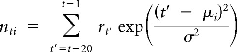 |
where μi = t − a,t − 3a, …, t − 19a was the center of the ith basis function, σ = a was the width of the basis functions, and a was 1 ms in time bin units. Depending on the form of h⃗, the probability that the model fired a spike could be suppressed by recent spiking (refractoriness) and/or facilitated (burstiness). The final term of Equation 1 was the constant input b, which set the spontaneous firing rate of the model. The nonlinear function f(·) was the logistic function f(x) = 1/(1 + exp) − x)).
The GLM was fitted by finding the parameters b, k⃗, and h⃗, which maximized the probability of the model given the data r⃗ and x⃗—the “posterior” distribution. We used an uncorrelated Gaussian prior for the parameters, with the scale determined by hyperparameters α and β:
 |
This high dimensional search was greatly facilitated by the fact that, due to properties of GLMs, the posterior probability is a concave function of the parameters, and therefore has a single, global maximum (Paninski et al., 2007). This maximum was located by iteratively reweighted least-squares (Nelder and Wedderburn, 1972). A type II maximum likelihood procedure was used to fit the hyperparameters (MacKay, 1992; Park and Pillow, 2011). For this procedure, the marginal likelihood was calculated using the Laplace approximation for the posterior distribution.
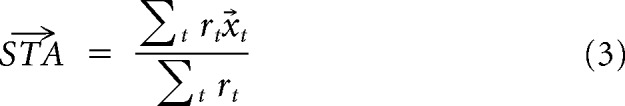
The input to the LNP model was the whisker stimulus time series. This was linearly filtered by convolution with a stimulus filter to produce a time-dependent coefficient zt, which was passed through a nonlinear “tuning function” to produce a time-dependent spiking probability p(spike|zt). For each single unit, the stimulus filter and tuning function were fitted to its response as previously described (Petersen et al., 2008). Depending on the form of this filter, the model could be sensitive to one of the canonical kinetic features (position, velocity, acceleration), to higher order derivatives of whisker motion, and/or to linear combinations of these. To estimate the stimulus filter, we computed the spike-triggered average (STA) of the spikes evoked by the nonrepeated white noise stimulus:
 |
The tuning function ensured a positive firing rate and accounted for potential nonlinear effects such as response saturation. To estimate the tuning function, a kernel density method was used to estimate the probability densities p(z) and p(z|spike), and the tuning function was estimated as p(spike|z) = p(z|spike)p(spike)/p(z), where p(spike) was estimated as the proportion of time bins containing a spike.
Prediction quality.
Once the best-fitting GLM/LNP parameters had been identified for a given unit, the next step was to assess the predictive power of the model. To do this, we used the neural responses evoked by the repeated stimulus sequences (white noise and texture) to measure the “experimental peristimulus time histogram (PSTH).” Then, we used the repeated stimulus sequence as input to the model and obtained its predicted response. By repeating this 50 times and averaging the responses, we obtained the “predicted PSTH.” To compare the quality of the prediction, the Pearson correlation coefficient between the experimental PSTH and predicted PSTH was calculated for each unit. This correlation coefficient was corrected for sampling error as described by Sahani and Linden (2003).
Feature analysis.
We characterized feature selectivity as previously described (Petersen et al., 2008). Briefly, we fitted a mixture model consisting of 1–3 Gaussians to each STA. An STA fit well by a single Gaussian (goodness of fit > 0.95) was classified as a position unit, by 2 Gaussians a velocity unit, and by 3 Gaussians an acceleration unit. Units with biphasic STAs were classified as position/velocity hybrids if the absolute difference in the integral of each phase divided by their sum was >0.1.
We examined the structure of the set of learned stimulus filters further by applying principal components analysis (PCA) to the set of stimulus filter vectors. We defined the relevant feature space as the hyperplane spanned by the eigenvectors accounting for 95% of the variance.
Results
Our primary aim was to develop a simple model that captures how whisker motion evokes spikes from primary whisker afferents. To be able to rigorously test the model, it was essential to record the responses of single units to multiple, identical repeats of controlled, whisker motion sequences and to control the statistics of the stimulus. To this end, we recorded the responses of single units from the trigeminal ganglion of anesthetized rats to controlled whisker deflection (N = 34). For each single unit, we used its responses to nonrepeated white noise whisker deflection to fit the parameters of the model. To test the accuracy of the model, we also recorded the unit's responses to repeated sequences of both white noise and texture (playback of whisker motion measured during active whisking of sandpaper by Wolfe et al., 2008). The SD of the white noise stimulus was the same as that of the texture stimulus. We start by reporting how the primary afferents responded to these whisker stimuli.
Response of primary afferents to whisker motion
Consistent with previous studies (Jones et al., 2004; Arabzadeh et al., 2005; Lottem and Azouz, 2011), primary afferents responded precisely and reproducibly to both white noise whisker motion (Fig. 1A–D) and texture-induced whisker motion (Fig. 1E–H). Spontaneous activity was almost absent (median 0.04 spikes/s, interquartile range across means (IQR) 0–0.14 spikes/s).
On average, firing rates were significantly higher for white noise than for texture (medians 12.0 spikes/s and 2.3 spikes/s, respectively, p = 7 × 10⁻⁷, Wilcoxon signed-rank test). There was substantial variability in the firing rates evoked by white noise (IQR 4.1–43.2 spikes/s) from different units (Figs. 1C,D, 2A). In contrast, the firing rates evoked by texture were more consistent (IQR 0.9–3.9 spikes).
Figure 2.

Comparison of primary afferent response to texture versus white noise. A, Each point shows the firing rate (averaged over 10 s stimulus presentation) evoked by white noise compared with that evoked by texture, for a given unit. B, Analogous comparison for spike- timing jitter.
As illustrated in Figure 1, C, D, G, and H, whisker motion typically evoked a series of temporally isolated firing episodes. Within each firing episode, spikes were precisely aligned across trials. To measure the spike timing precision, we measured the differences in spike time across trials within each episode (Montemurro et al., 2007). The median SD of these differences (“jitter”) was 0.15 ms for white noise (IQR 0.130–0.23 ms) and 0.22 ms for texture (IQR 0.17–0.30 ms) (Fig. 2B). For every unit in our sample, the jitter was <1 ms.
We found diversity in how different primary afferents responded to the same white noise stimulus (Figs. 2, 3). Units differed not only in evoked firing rate (Fig. 2A) but also in the temporal pattern of the evoked response (Fig. 3A). This suggests that different units might be tuned to different kinetic features of whisker motion (position, velocity, etc.). To test this, we cross-correlated the PSTH of each unit with the white noise sequence that evoked it, and also with the first derivative of the whisker motion (“velocity”) and the second derivative (“acceleration”). This analysis revealed diversity in the feature selectivity of the primary afferent population (Fig. 3B). Some units correlated best with velocity in the rostral direction (unit 28) or caudal direction (unit 1); others correlated best with position (unit 26) or with acceleration (unit 25). To test whether units might be sensitive to more complex kinetic features, we computed STAs (Fig. 3F). As a comparison, the STAs expected for ideal position, velocity, and acceleration-sensitive units stimulated with white noise are shown in Figure 3C—E (Petersen et al., 2008). We did find units with STAs similar to the ideal types (Fig. 3F). However, most units were hybrids of the ideal types, with the single most common type of STA being biphasic (29/34 units, 85%; Fig. 3G). This indicates that most primary afferents are not exclusively sensitive to the canonical kinetic features of position, velocity, or acceleration, but rather are sensitive to multiple features.
Figure 3.

Diverse responses in the population of primary afferents. A, PSTHs (1 ms bins, normalized to each unit's maximum firing rate) of all recorded units evoked by white noise. B, For each unit, correlation coefficient between the PSTH and position, velocity, and acceleration of the white noise. C–E, STAs for ideal position, velocity, and acceleration-sensitive units. F, STAs for each recorded unit. G, STAs classified by fitting to a mixture of Gaussians model (Petersen et al., 2008). P/V denotes position/velocity hybrids (see Materials and Methods).
Next, we tested whether there were interactions between spikes in the evoked response. In the simplest type of spike train, a Poisson process, the mean of the number of spikes that occur in a particular time window (the “spike count”) is equal to its variance. We tested this (using 20 ms time windows) and found that the spike count variance was typically lower than its mean (see Fig. 5C1,C2). This indicates that, for both types of stimulus, the evoked spike trains were more regular than expected from a Poisson process. The variance frequently tracked the theoretical minimum value consistent with the mean (Fig. 5C1,C2, scalloping). In sum, we found that responses of primary afferents were characterized by reliability, high temporal precision, sub-Poisson variability, and diverse stimulus selectivity. The challenge was to capture these characteristics with a simple model.
Figure 5.

PSTH prediction performance for the GLM: single-unit examples. A1, PSTH of an example unit (black line) evoked by white noise, compared with PSTH predicted by the GLM model with parameters shown in Figure 4C1–D1 (gray line). B1, Corresponding data for the texture stimulus (same unit as A1). C1, Variance of spike count across trials (20 ms time window) plotted against its mean (same unit as A1). D1, Corresponding data for the GLM model. A2–D2, Analogous results for a second example unit.
GLM of response to whisker motion
We used the responses of each primary afferent to 500 s of nonrepeated white noise to fit the parameters of the GLM, schematized in Figure 4A.
Figure 4.

Model structure and parameter fitting. A, Schematic of the GLM. The linear filters k⃗ and h⃗ are convolved with the whisker stimulus and spike history, respectively. The resulting coefficients are summed with the constant b and passed through the nonlinear function f(·) to produce the time-dependent probability of a spike. B1, Stimulus filter for an example unit. C1, The stimulus filter convolved with the white noise autocorrelation (black line), compared with the unit's STA (gray line). D1, The unit's spike feedback filter. B2–D2, Corresponding results for a second example unit.
The aim of the GLM was to capture the transformation between sensory stimulus and spike train response. In any time bin, a GLM fires a spike with a certain probability. This probability depends on two principal elements. The first is a time-independent stimulus filter: the parameters of this filter determine the kinetic feature to which the model is sensitive. For example, the stimulus filter shown in Figure 4A approximately differentiates the stimulus, and makes the model sensitive to instantaneous velocity. The filters shown in Figure 3, C and E, make the model sensitive to position and acceleration, respectively. The second element of the GLM is a “spike history filter.” This makes the response of the model depend not only the stimulus but also on the spikes fired in the recent past. For example, the filters shown in Figure 4, D1 and D2, produce large negative values immediately following a spike, briefly silencing the model (refractoriness).
Any model can be fitted to data, but there is no guarantee that the best-fitting model fully captures the neuron's encoding behavior. It was therefore crucial to rigorously test the GLM. To this end, we first asked whether the GLM could accurately predict the response evoked by a sequence of white noise. To do this, we used experimental recordings of the unit's response to 50 repetitions of the same 10 s sequence of repeated white noise (a sequence not used for GLM parameter fitting) to obtain a PSTH. We then used this same sequence of white noise as input to the GLM and registered its spike train output (bin size 2 ms). By repeating this 50 times, and averaging the responses, we obtained a predicted PSTH. We typically found a remarkably close match between the experimental and predicted PSTHs (Fig. 5A1,A2). The GLM accurately captured both the timing of the PSTH peaks and their amplitudes. We quantified the prediction quality by calculating a modified Pearson correlation coefficient between the predicted and experimental PSTHs (see Materials and Methods). For the example units of Figure 5, A1 and A2, the prediction coefficients were 0.95 and 0.93, respectively.
To test whether these results were representative, we fitted GLMs to all single units in our sample and tested their prediction quality as above. We found that GLMs generally provided excellent fits to the PSTH evoked by white noise (Fig. 6A,B). The median prediction correlation coefficient was 0.92 (IQR 0.90–0.94).
Figure 6.

PSTH Prediction performance of the GLM: population data. A, Each point shows the prediction quality (correlation coefficient between actual and predicted PSTH) for white noise compared with that for texture, for a given unit; 1 ms bins. B, Effect of spike feedback term on PSTH prediction: correlation coefficient between actual and predicted PSTH with spike feedback compared with that without spike feedback for a given unit. Results computed for white noise.
Although these results were encouraging, the statistics of white noise whisker motion differ from those of natural exploratory whisking (Hipp et al., 2006; Fig. 1A,B,E,F). This is significant since, in general, the best-fitting parameters of a model depend on the statistics of the data used for parameter estimation. There is no guarantee that a model fitted on white noise data will extrapolate well to stimuli with different statistics (Talebi and Baker, 2012). Hence it was important to test whether the GLM extrapolated to more naturalistic whisker motion. To this end, we tested how well a GLM (with parameters fitted to white noise data only) could predict the response to playback of whisker motion generated by active exploration of a textured surface (see Materials and Methods). As above, we used the texture sequence as input to the GLM and obtained a predicted PSTH, which we compared with the corresponding experimental PSTH. We found that the model PSTHs matched the experimental PSTH remarkably well. For the example units of Figure 5, B1 and B2, the prediction coefficients were 0.78 and 0.85, respectively. This was typical (Fig. 6A): the median prediction coefficient was 0.86 (IQR 0.71–0.89).
The accuracy of the predicted PSTHs suggests that GLMs accurately captured the response of primary afferents to our whisker motion stimuli. This indicates that useful insight into how these neurons encode whisker motion might be obtained by examining the parameters of the model. Figure 4 shows both stimulus filters and spike history filters for two example units. The stimulus filters (Fig. 4B1,B2) indicate that the units responded most strongly to precisely timed stimulus features occurring 4–8 ms before the current time. To facilitate interpretation of the stimulus filters, we multiplied each stimulus filter vector by the covariance matrix of the white noise stimulus. We found that the smoothed stimulus filters were similar, although not identical, to the corresponding STAs (Fig. 4C1,C2). This indicates that the kinetic feature selectivity revealed by GLM and STA approaches were consistent, but that the GLM was able to uncover stimulus filter structure on a significantly finer timescale. This was important for the ability of GLMs to account for the fine temporal structure of the PSTHs.
For both units, the spike history filters (Fig. 4D1,D2) were large and negative for recently occurring spikes, and approached zero for spikes occurring >10 ms in the past. This enforced a refractory period: similar spike history filters were found for all units in our sample. To test the importance of the spike history component of the GLM, we refitted the model without the spike history filter h⃗ (Eq. 1). As shown in Figure 6B, the performance of this model variant was significantly inferior to that of the full model (median prediction qualities 0.86 and 0.92; p = 2 × 10⁻⁶, Wilcoxon signed-rank test).
To test whether the GLM was able to capture the spike-timing precision of the primary afferents, we repeated the parameter fitting process using a range of time bins (0.1–10 ms) and quantified performance, as above, by computing a correlation coefficient between experimental and predicted PSTHs (Fig. 7A). The most accurate prediction was observed for bin sizes of 2 ms (median prediction coefficient for white noise 0.92; for texture 0.86). However, the PSTH prediction was accurate for a range of bin sizes; for white noise, exceeding a median prediction coefficient of 0.8 for bin sizes from 0.25 to 4 ms. Thus, the GLM was able to account accurately for submillisecond spike-timing precision.
Figure 7.

Timing precision of PSTH prediction. A, Correlation coefficient (median across units) between recorded and predicted PSTHs for white noise and texture, as a function of spike time bin size. Data shown both for GLM and LNP models. Bars denote SEM, computed by bootstrap resampling. B, Example of PSTH evoked by white noise (black line above the x-axis) compared with predicted PSTH from GLM (black line below) and LNP model (gray line below).
To get further insight into why the predictions of the GLM were accurate even at submillisecond timescales, we compared the prediction performance of the GLM to that of an STA-based LNP model (see Materials and Methods). The LNP model is similar to the GLM in that its output is a nonlinear function of a filter convolved with the sensory stimulus. However, it differs in that there is no spike feedback mechanism. We found that, for larger bin sizes (6–8 ms), prediction performance was similar for GLM and LNP (both medians 0.78 at 6 ms; Fig. 7A). However, for small bin sizes, the GLM showed a substantial advantage (medians 0.88 and 0.62 for GLM and LNP, respectively, at 0.5 ms). The LNP model was able to predict quite well the occurrence of major peaks in the PSTH, but, in contrast to the GLM, the LNP model was unable to accurately predict their precise temporal structure (Fig. 7B). Together, these results indicate the importance of fitting the stimulus filter at a timescale finer than the correlation timescale of the stimulus and the importance of taking spike feedback into account.
As noted above, a good model should be able to account not only for the mean response of a neuron to the stimulus (the PSTH) but also for higher order statistical structure of the evoked spike trains. Our next aim was to test whether the GLM could account for the sub-Poisson variance of the evoked response (Fig. 5C,D). To this end, we used the GLM fitted to each afferent to generate spike trains evoked by white noise. We then used these responses to generate scatter plots of mean spike count versus its variance as above (Fig. 5C2–D2; 20 ms time window). We found that the model data exhibited similar scalloped structure to that of the experimental data.
To summarize, we found that GLMs successfully captured a number of fundamental characteristics of primary afferents: they accurately predicted the response of primary afferents to white noise, they generalized accurately to texture, they captured submillisecond spike timing precision, and they accounted for sub-Poisson spike train statistics.
Feature representation
The results of the previous section imply that the best-fitting stimulus filter of a GLM accurately captured the stimulus selectivity of the corresponding primary afferent. Our final aim was to use this as a basis for getting insight into the space of whisker motion features represented by primary whisker afferents. In particular, we asked whether it might be possible to capture the variety of the stimulus filters by a lower dimensional description. To test this, we applied PCA to the set of GLM stimulus filters. To obtain robust results, we first smoothed the stimulus filters by multiplication with the autocorrelation matrix of the white noise (Fig. 4C). We found that a small number of principal components (PCs) captured almost all the variance in the stimulus filters (Fig. 8A). The first PC explained 81% of the variance, the first two PCs explained 94%, and the first three PCs explained 99%. This indicates that the diversity of stimulus selectivity in the population of primary afferents could be accurately described by a low (2–3D) dimensional “filter space.”
Figure 8.

Kinetic feature space encoded by the primary afferent population. A, Proportion of variance of stimulus filters explained by 1–4 PCs in order of decreasing eigenvalue. B, The first three PCs. C, Smoothed stimulus filters for each primary afferent plotted at its location in the space spanned by PCs 1 and 2 (gray lines). Superimposed are the stimulus features corresponding to different locations in the space, as detailed in the main text (black). D, Corresponding plot for PCs 1 and 3.
Since the filter space was low dimensional, it was possible to directly visualize its structure. The first and second PCs were both biphasic (Fig. 8B1,B2). To visualize the space spanned by these two PCs, we systematically generated filters composed of different linear combinations of them (Fig. 8C, gray lines). For example, filters along the x-axis were proportional to the first PC and filters along the main diagonal to the sum of the two PCs. Different directions in this space corresponded to selectivity to different kinetic features. Positive, monophasic filters (compare Figs. 8C, top middle, 3C) imply tuning to whisker position and preference for the caudal direction and negative monophasic filters (bottom middle) for the rostral direction. Biphasic filters imply tuning to whisker velocity (compare Fig. 3D) either in the caudal direction (Fig. 8C, top left) or, if the sign is reversed, in the rostral direction (bottom right). Most regions of the space contained biphasic filters different to the canonical ones of Figure 3, C and D, in that the two phases were of unequal amplitude (Fig. 8C, left middle and right middle). Such filters reflect sensitivity to both position and velocity (Petersen et al., 2008). The third PC (Fig. 8B3) was triphasic. Including this PC as a third dimension (Fig. 8D, gray lines) thus produced also triphasic filters, sensitive to acceleration (compare Fig. 3E).
For each unit in our database, we computed the projection of its stimulus filter onto the first three PCs and plotted the stimulus filter in the corresponding location of the PC1–PC2 plane (Fig. 8C, black lines) and PC1–PC3 plane (Fig. 8D, black lines). The stimulus filters were spread relatively widely. Thus, although the space of features was low dimensional, there was nonetheless diversity between units. Approximately, the primary afferent units “tiled” the filter space.
Discussion
To identify a neural code, it is necessary to determine the sensory events that are encoded by spikes. For primary whisker afferents, previous research has shown that spikes evoked by whisker motion exhibit high temporal precision, and that firing rate is modulated by a number of parameters of whisker deflection, including the location, direction, and velocity (Zucker and Welker, 1969; Gibson and Welker, 1983; Lichtenstein et al., 1990; Jones et al., 2004; Arabzadeh et al., 2005). In some cases, it has also been shown that the response of primary afferents to complex tactile stimuli can be predicted by mathematical models (Mitchinson et al., 2004, 2008; Arabzadeh et al., 2005; Lottem and Azouz, 2011). Our study builds on this work by seeking to develop a simple, but general, model that captures this and other fundamental characteristics of primary afferent responses. We found that a GLM not only accurately predicted the response of primary afferents to white noise whisker motion, but also accurately predicted their response to texture-induced whisker motion. The GLM captured primary afferent submillisecond spike-timing precision; it also captured their sub-Poisson spike train statistics. Analysis of the model indicated that primary afferents approximately tile a low-dimensional feature space.
GLM
The GLM (Paninski, 2004; Truccolo et al., 2005) consists of a time-independent stimulus filter and a spike history filter. Its elegant mathematical structure is conducive to effective parameter fitting (Paninski et al., 2007), but its assumptions are potentially limiting. For barrel cortical neurons, multiple stimulus filters are typically necessary, and time-dependent adaptive processes exert a marked effect on the evoked response (Maravall et al., 2007; Lundstrom et al., 2010; Estebanez et al., 2012). For primary afferents, slow adaptive mechanisms are necessary to capture phase shifts exhibited by some neurons in response to periodic whisker deflections superimposed on a DC offset (Lottem and Azouz, 2011). It is therefore striking that the GLM was sufficient to accurately capture the evoked responses to complex whisker motion for the bulk of our units, even though our texture-induced whisker motion stimulus had substantial low frequency content (Fig. 1E). However, it should be noted that the average prediction accuracy for texture, while high (median 0.86), was lower than that for white noise (median 0.92). Moreover, there was a small minority of primary afferents that were less well described. It is possible that a more complex model, taking slow time course features of the stimulus into account, might be even more accurate. Indeed, Lottem and Azouz (2011) showed that a biomechanical model with a novel dynamic rectification mechanism was able to account for phase shifts not captured by simpler models. An interesting challenge for future theoretical work is to extend the GLM to capture slow time course stimulus effects.
Precision of spike timing
We found, consistent with previous studies (Jones et al., 2004; Arabzadeh et al., 2005; Storchi et al., 2012) that primary whisker afferents responded with remarkably high timing precision: the median jitter was 0.2 ms. The significance is that it endows neurons with a high capacity for transmitting information (Petersen et al., 2009; Petersen, 2013). Submillisecond timing precision is challenging to reproduce in a model when the correlation timescale of the stimulus is longer: here, the full-width at half-maximum of the white noise autocorrelation was 5 ms. Yet, we found that the GLM parameter-fitting procedure was able to accurately predict the units' responses at submillisecond precision, resolving stimulus features at higher precision than the STA.
Predicting the response to complex whisker motion
White noise is a valuable stimulus for model fitting, since it explores a large stimulus space in an efficient and unbiased manner (Jones et al., 2004; Arabzadeh et al., 2005; Maravall et al., 2007; Montemurro et al., 2007; Petersen et al., 2008; Lottem and Azouz, 2011; Estebanez et al., 2012). However, the statistics of white noise differ from those of natural whisker motion (Hipp et al., 2006). To test whether the model predicted PSTHs evoked by more naturalistic whisker motion, we used a playback approach (Arabzadeh et al., 2005) to reproduce whisker motion recorded optically while rats actively whisked a sandpaper-textured surface (Wolfe et al., 2008). We found that, although the GLM parameters were fitted using only white noise data, the model accurately predicted the texture-induced PSTHs. Other types of mathematical model also predict texture-induced responses (Arabzadeh et al., 2005; Lottem and Azouz, 2011). The advantage of the GLM is that, for any dataset, there is a global optimum solution to the parameters that can be automatically learned. Moreover, its simplicity is conducive to insight into the neural code (see below). An important challenge for future research will be to test the model in the awake, behaving animal. However, since multiple trials of identical whisker motion sequences cannot be delivered under these conditions, the present PSTH prediction approach is inapplicable and new methods will be required.
Capturing higher order spike train structure
For the simplest type of spike train, a Poisson process, the PSTH is a sufficient statistical description of a neuron's response (Rieke et al., 1997). However, we found that the spike trains evoked by primary afferents were significantly more regular than Poisson. Non-Poisson structure cannot be captured by LNP models, which assume that spikes are generated independently, but an advantage of the GLM is that spike interaction effects can be learned from data (Pillow et al., 2005). We found that GLMs could account for the quadratic (“scalloped”) relationship between spike count variance and spike count mean (Fig. 5D1,D2). This was due to the spike history mechanism of the GLM. The spike history filter was typically strongly negative just after a spike. This induced a refractory effect. Within a short time window neurons thus fired at most one spike, with probability p. It follows that the variance of the spike count within this window is the quadratic function p (1 − p) (de Ruyter van Steveninck et al., 1997).
Feature selectivity of primary afferents
Arabzadeh et al. (2005) showed that, for some primary afferents, the PSTH evoked by texture-induced whisker motion could be accurately predicted by tuning to instantaneous whisker velocity. We found that 85% of units did indeed exhibit biphasic stimulus filters indicative of velocity tuning. Yet we also found considerable diversity. Diversity has been consistently reported under a variety of experimental paradigms (Zucker and Welker, 1969; Gibson and Welker, 1983; Lichtenstein et al., 1990; Shoykhet et al., 2000; Szwed et al., 2003). We found that other afferents exhibited monophasic position filters or triphasic acceleration filters. The most common case was a biphasic stimulus filter, sensitive to both position and velocity. This is consistent with mechanotransduction models, where forces applied to the whisker follicle induce stresses/strains within the visco-elastic tissues of the FSC: these forces are gated by ion channels in the mechanoreceptor membrane (Mitchinson et al., 2004, 2008; Lottem and Azouz, 2011). Mitchinson et al. (2004) reported that, to first approximation, the strain within the FSC is proportional to a linear combination of whisker position and whisker velocity. Diversity in the primary afferent population may reflect variation in morphological types of mechanoreceptor (Rice et al., 1986), in location of the mechanoreceptors within the FSC (Ebara et al., 2002; Mitchinson et al., 2004) and in expression of voltage-dependent membrane currents. The stimulus filters that we found were similar to those previously reported in the ventroposterior medial thalamus (Petersen et al., 2008), suggesting that the primary afferents fundamentally shape feature selectivity in the whisker system.
Feature space encoded by primary afferents
To investigate the “space” of features that the primary afferent population encodes, we applied principal components analysis to the stimulus filters. Ninety-nine percent of the variance could be explained by three dimensions. Dimensions 1–2 accounted for sensitivity to position and velocity; dimension 3 reflected also acceleration. Thus, primary afferents were sensitive to different linear combinations of position, velocity, and acceleration, with the major weight carried by the former two. Our results imply that the population approximately tiles this feature space. A caveat is that we only studied whisker motion in the rostrocaudal direction. Primary afferents are typically direction dependent (Zucker and Welker, 1969), implying that the complete feature space will include additional dimensions to capture components of whisker motion in the ventrodorsal direction.
On the face of it, this way of encoding a sensory input seems inefficient. In principle, a 3D space could be represented by just three “Cartesian” neurons, with linearly independent stimulus filters. However, the whisker follicle is innervated by many times more neurons than this scheme would require. A drawback of the Cartesian scheme is that each neuron must accurately encode its corresponding coordinate, and transmitting a real-valued coordinate (e.g., through the spike count in a given time window) takes time. Instead, the primary whisker afferents appear to represent a low-dimensional feature space as a high (∼200 D) dimensional, distributed population code. This may allow the system to transmit which feature has occurred by single spikes from the appropriate subpopulation of neurons and thereby achieve rapid information transfer to the CNS (Chase, 2012).
Conclusion: neural coding in whisker primary afferents
Our results suggest that the response of primary afferents to complex whisker motion can be comprehensively captured by a surprisingly simple model based on stimulus filtering and spike feedback. Whisker motion is encoded as an overcomplete representation of, primarily, whisker position and whisker velocity.
Footnotes
This work was supported by the CARMEN e-science project (EPSRC Grant EP/E002331/1), Biotechnology and Biological Sciences Research Council Grant BB/G020094/1, Wellcome Trust Institutional Strategic Support Fund award (097820) to the University of Manchester, and the Lord Alliance Foundation. We thank M. Montemurro for valuable discussions and D. Feldman and J. Wolfe for sharing their whisker motion data and for valuable discussions.
The authors declare no competing financial interests.
References
- Arabzadeh E, Zorzin E, Diamond ME. Neuronal encoding of texture in the whisker sensory pathway. PLoS Biol. 2005;3:e17. doi: 10.1371/journal.pbio.0030017. [DOI] [PMC free article] [PubMed] [Google Scholar]
- Bale MR, Petersen RS. Transformation in the neural code for whisker deflection direction along the lemniscal pathway. J Neurophysiol. 2009;102:2771–2780. doi: 10.1152/jn.00636.2009. [DOI] [PMC free article] [PubMed] [Google Scholar]
- Chase SM. Single spikes may suffice. J Neurophysiol. 2012;108:1808–1809. doi: 10.1152/jn.00507.2012. [DOI] [PubMed] [Google Scholar]
- de Ruyter van Steveninck RR, Lewen GD, Strong SP, Koberle R, Bialek W. Reproducibility and variability in neural spike trains. Science. 1997;275:1805–1808. doi: 10.1126/science.275.5307.1805. [DOI] [PubMed] [Google Scholar]
- Diamond ME, Arabzadeh E. Whisker sensory system–from receptor to decision. Prog Neurobiol. 2013;103:28–40. doi: 10.1016/j.pneurobio.2012.05.013. [DOI] [PubMed] [Google Scholar]
- Ebara S, Kumamoto K, Matsuura T, Mazurkiewicz JE, Rice FL. Similarities and differences in the innervation of mystacial vibrissal follicle-sinus complexes in the rat and cat: a confocal microscopic study. J Comp Neurol. 2002;449:103–119. doi: 10.1002/cne.10277. [DOI] [PubMed] [Google Scholar]
- Estebanez L, El Boustani S, Destexhe A, Shulz DE. Correlated input reveals coexisting coding schemes in a sensory cortex. Nat Neurosci. 2012;15:1691–1699. doi: 10.1038/nn.3258. [DOI] [PubMed] [Google Scholar]
- Gibson JM, Welker WI. Quantitative studies of stimulus coding in first-order vibrissa afferents of rats. 1. Receptive field properties and threshold distributions. Somatosens Res. 1983;1:51–67. doi: 10.3109/07367228309144540. [DOI] [PubMed] [Google Scholar]
- Hipp J, Arabzadeh E, Zorzin E, Conradt J, Kayser C, Diamond ME, König P. Texture signals in whisker vibrations. J Neurophysiol. 2006;95:1792–1799. doi: 10.1152/jn.01104.2005. [DOI] [PubMed] [Google Scholar]
- Jones LM, Depireux DA, Simons DJ, Keller A. Robust temporal coding in the trigeminal system. Science. 2004;304:1986–1989. doi: 10.1126/science.1097779. [DOI] [PMC free article] [PubMed] [Google Scholar]
- Khatri V, Bermejo R, Brumberg JC, Keller A, Zeigler HP. Whisking in air: encoding of kinematics by trigeminal ganglion neurons in awake rats. J Neurophysiol. 2009;101:1836–1846. doi: 10.1152/jn.90655.2008. [DOI] [PMC free article] [PubMed] [Google Scholar]
- Leiser SC, Moxon KA. Responses of trigeminal ganglion neurons during natural whisking behaviors in the awake rat. Neuron. 2007;53:117–133. doi: 10.1016/j.neuron.2006.10.036. [DOI] [PubMed] [Google Scholar]
- Lichtenstein SH, Carvell GE, Simons DJ. Responses of rat trigeminal ganglion neurons to movements of vibrissae in different directions. Somatosens Mot Res. 1990;7:47–65. doi: 10.3109/08990229009144697. [DOI] [PubMed] [Google Scholar]
- Lottem E, Azouz R. A unifying framework underlying mechanotransduction in the somatosensory system. J Neurosci. 2011;31:8520–8532. doi: 10.1523/JNEUROSCI.6695-10.2011. [DOI] [PMC free article] [PubMed] [Google Scholar]
- Lundstrom BN, Fairhall AL, Maravall M. Multiple timescale encoding of slowly varying whisker stimulus envelope in cortical and thalamic neurons in vivo. J Neurosci. 2010;30:5071–5077. doi: 10.1523/JNEUROSCI.2193-09.2010. [DOI] [PMC free article] [PubMed] [Google Scholar]
- MacKay DJC. Bayesian interpolation. Neural Comput. 1992;4:415–447. doi: 10.1162/neco.1992.4.3.415. [DOI] [Google Scholar]
- Maravall M, Petersen RS, Fairhall AL, Arabzadeh E, Diamond ME. Shifts in coding properties and maintenance of information transmission during adaptation in barrel cortex. PLoS Biol. 2007;5:e19. doi: 10.1371/journal.pbio.0050019. [DOI] [PMC free article] [PubMed] [Google Scholar]
- Mitchinson B, Gurney KN, Redgrave P, Melhuish C, Pipe AG, Pearson M, Gilhespy I, Prescott TJ. Empirically inspired simulated electro-mechanical model of the rat mystacial follicle-sinus complex. Proc Biol Sci. 2004;271:2509–2516. doi: 10.1098/rspb.2004.2882. [DOI] [PMC free article] [PubMed] [Google Scholar]
- Mitchinson B, Arabzadeh E, Diamond ME, Prescott TJ. Spike-timing in primary sensory neurons: a model of somatosensory transduction in the rat. Biol Cybern. 2008;98:185–194. doi: 10.1007/s00422-007-0208-7. [DOI] [PubMed] [Google Scholar]
- Montemurro MA, Panzeri S, Maravall M, Alenda A, Bale MR, Brambilla M, Petersen RS. Role of precise spike timing in coding of dynamic vibrissa stimuli in somatosensory thalamus. J Neurophysiol. 2007;98:1871–1882. doi: 10.1152/jn.00593.2007. [DOI] [PubMed] [Google Scholar]
- Nelder JA, Wedderburn RWM. Generalized linear models. J R Statist Soc Ser A. 1972;135:370–384. doi: 10.2307/2344614. [DOI] [Google Scholar]
- Paninski L. Maximum likelihood estimation of cascade point-process neural encoding models. Network. 2004;15:243–262. doi: 10.1088/0954-898X/15/4/002. [DOI] [PubMed] [Google Scholar]
- Paninski L, Pillow JW, Lewi J. Statistical models for neural encoding, decoding, and optimal stimulus design. Prog Brain Res. 2007;165:493–507. doi: 10.1016/S0079-6123(06)65031-0. [DOI] [PubMed] [Google Scholar]
- Park M, Pillow JW. Receptive field inference with localized priors. PLoS Comput Biol. 2011;7:e1002219. doi: 10.1371/journal.pcbi.1002219. [DOI] [PMC free article] [PubMed] [Google Scholar]
- Petersen RS. Role of temporal spike patterns in neural codes. In: Quiroga RQ, Panzeri S, editors. Principles of neural coding. Boca Raton, FL: CRC; 2013. [Google Scholar]
- Petersen RS, Brambilla M, Bale MR, Alenda A, Panzeri S, Montemurro MA, Maravall M. Diverse and temporally precise kinetic feature selectivity in the VPm thalamic nucleus. Neuron. 2008;60:890–903. doi: 10.1016/j.neuron.2008.09.041. [DOI] [PubMed] [Google Scholar]
- Petersen RS, Panzeri S, Maravall M. Neural coding and contextual influences in the whisker system. Biol Cybern. 2009;100:427–446. doi: 10.1007/s00422-008-0290-5. [DOI] [PubMed] [Google Scholar]
- Pillow JW, Paninski L, Uzzell VJ, Simoncelli EP, Chichilnisky EJ. Prediction and decoding of retinal ganglion cell responses with a probabilistic spiking model. J Neurosci. 2005;25:11003–11013. doi: 10.1523/JNEUROSCI.3305-05.2005. [DOI] [PMC free article] [PubMed] [Google Scholar]
- Rice FL, Mance A, Munger BL. A comparative light microscopic analysis of the sensory innervation of the mystacial pad. I. Innervation of vibrissal follicle-sinus complexes. J Comp Neurol. 1986;252:154–174. doi: 10.1002/cne.902520203. [DOI] [PubMed] [Google Scholar]
- Rieke F, Warland D, de Ruyter van Steveninck R, Bialek W. Spikes: exploring the neural code. Cambridge, MA: MIT; 1997. [Google Scholar]
- Sahani M, Linden J. How linear are auditory cortical responses? Adv Neural Inf Process Syst. 2003;15:125–132. [Google Scholar]
- Schwartz O, Pillow JW, Rust NC, Simoncelli EP. Spike-triggered neural characterization. J Vis. 2006;6(4):484–507. doi: 10.1167/6.4.13. [DOI] [PubMed] [Google Scholar]
- Shoykhet M, Doherty D, Simons DJ. Coding of deflection velocity and amplitude by whisker primary afferent neurons: implications for higher level processing. Somatosens Mot Res. 2000;17:171–180. doi: 10.1080/08990220050020580. [DOI] [PubMed] [Google Scholar]
- Storchi R, Bale MR, Biella GE, Petersen RS. Comparison of latency and rate coding for the direction of whisker deflection in the subcortical somatosensory pathway. J Neurophysiol. 2012;108:1810–1821. doi: 10.1152/jn.00921.2011. [DOI] [PMC free article] [PubMed] [Google Scholar]
- Szwed M, Bagdasarian K, Ahissar E. Encoding of vibrissal active touch. Neuron. 2003;40:621–630. doi: 10.1016/S0896-6273(03)00671-8. [DOI] [PubMed] [Google Scholar]
- Talebi V, Baker CL., Jr Natural versus synthetic stimuli for estimating receptive field models: a comparison of predictive robustness. J Neurosci. 2012;32:1560–1576. doi: 10.1523/JNEUROSCI.4661-12.2012. [DOI] [PMC free article] [PubMed] [Google Scholar]
- Truccolo W, Eden UT, Fellows MR, Donoghue JP, Brown EN. A point process framework for relating neural spiking activity to spiking history, neural ensemble, and extrinsic covariate effects. J Neurophysiol. 2005;93:1074–1089. doi: 10.1152/jn.00697.2004. [DOI] [PubMed] [Google Scholar]
- Wolfe J, Hill DN, Pahlavan S, Drew PJ, Kleinfeld D, Feldman DE. Texture coding in the rat whisker system: slip-stick versus differential resonance. PLoS Biol. 2008;6:e215. doi: 10.1371/journal.pbio.0060215. [DOI] [PMC free article] [PubMed] [Google Scholar]
- Zucker E, Welker WI. Coding of somatic sensory input by vibrissae neurons in the rat's trigeminal ganglion. Brain Res. 1969;12:138–156. doi: 10.1016/0006-8993(69)90061-4. [DOI] [PubMed] [Google Scholar]