Behavior and neural basis of near-optimal visual search

Abstract

The ability to search efficiently for a target in a cluttered environment is one of the most remarkable functions of the nervous system. This task is difficult under natural circumstances, as the reliability of sensory information can vary greatly across space and time and is typically a priori unknown to the observer. In contrast, visual-search experiments commonly use stimuli of equal and known reliability. In a target detection task, we randomly assigned high or low reliability to each item on a trial-by-trial basis. An optimal observer would weight the observations by their trial-to-trial reliability and combine them using a specific nonlinear integration rule. We found that humans were near-optimal, regardless of whether distractors were homogeneous or heterogeneous and whether reliability was manipulated through contrast or shape. We present a neural-network implementation of near-optimal visual search based on probabilistic population coding. The network matched human performance.

Searching for a target among distractors is a task of great ecological relevance, whether for an animal trying to detect a camouflaged predator or for a student looking for a note on a cluttered desk. It is well known that the difficulty of detecting a target depends on the number of items in a scene (set size)^1–6, target-distractor similarity⁷ and distractor heterogeneity^7–10. However, an important aspect has largely been ignored in previous work: the effect of differential stimulus reliability. In realistic search scenes, some stimuli provide more reliable information than others, for example, as a result of differences in contrast, distance, shape or blur. In laboratory search tasks, however, such parameters are usually held constant across items and trials.

Varying reliability on a trial-by-trial basis is a key manipulation when studying whether the human brain performs probabilistically optimal (Bayesian) inference. This is because an optimal observer weights more reliable pieces of sensory evidence more heavily when making a perceptual judgment. For example, when two noisy sensory cues about a single underlying stimulus have to be combined, an optimal observer assigns higher weight to the cue that, on that trial, is most reliable. Humans follow this strategy closely and, as a result, they perform near-optimally in such tasks^11,12. The success of probabilistic models of cue combination and other perceptual tasks indicates that the brain utilizes knowledge of stimulus uncertainty and suggests that it computes with probability distributions. The neural basis of computing with probability distributions has become the subject of theoretical¹³ and physiological¹⁴ studies.

A major limitation of studies demonstrating near-optimal perception in the presence of sensory noise is that most of them use relatively simple tasks that require observers to infer a physical feature of a single stimulus item. To determine how prevalent near-optimal inference in perception is, it is necessary to explore tasks with more complex structures. In visual target detection, each display contains multiple items and their features are not of interest by themselves but only serve to inform the more abstract, categorical judgment of target presence. It is therefore considerably more complex than cue combination. We report here that, when judging target presence, humans take into account the reliabilities of the observations on a single trial in a near-optimal manner.

We also created a neural implementation of Bayes-optimal visual search. Although previous studies have focused on connecting search behavior to the activity of single neurons or pools of identical neurons^15,16, our implementation is based on the activity of a population of neurons with different tuning properties. Such populations can simultaneously encode a stimulus value and its reliability, thereby allowing for computation with probability distributions on a single trial.

Our results and model are not the first attempt to approach visual search from a probabilistic perspective^{1,6,8,15–18}. However, we extend previous ideas in three fundamental ways. First, we consider situations in which the reliability of the visual information varies unpredictably in and across displays. This is a common occurrence in the real world and a strong test of probabilistic models of perception. Second, we deal with the difficult problem of how information should be combined across unknown distractor values and spatial locations, a problem that involves a type of inference known as marginalization. Finally, we provide a neural implementation of near-optimal visual search that can account for our data and can deal with the marginalization problem.

RESULTS

Theory

We used a task in which subjects were presented briefly with an array of N oriented bars (Fig. 1a) and reported whether a target was present, regardless of its location. The target was a bar of fixed orientation, denoted s_T, which was present with a probability of 0.5. In separate experiments, the distractor orientation was drawn from either a delta function, in which all distractors have the same orientation, denoted s_D (we call this the case of homogeneous distractors; Fig. 1a), or a uniform distribution on orientation space [0,180°) (we call this the case of heterogeneous distractors; Fig. 1a). Notably, each item was independently assigned high or low reliability.

Figure 1.

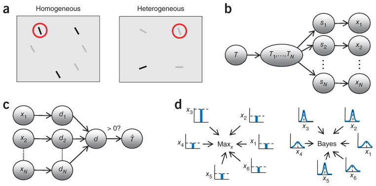
Reliability and inference in visual search. (a) Search under unequal reliabilities. Stimulus reliability is controlled by contrast, but the target (red circle) is defined only by orientation. Left, homogeneous distractors. Right, heterogeneous distractors. (b) Statistical structure of the task (generative model). Arrows indicate conditional dependencies. T, global target presence; T_i, local target presence; s_i, stimulus orientation; x_i, noisy observation. In the neural formulation, x_i is replaced by a pattern of neural activity, r_i. (c) The optimal decision process for inferring target presence inverts the generative model. d_i, local log likelihood ratio of target presence; d, global log likelihood ratio. The sign of d determines the decision and its absolute value reflects confidence. (d) Left, max_x model applied to a homogeneous-distractor display as in a. At each location, an orientation detector produces a response x_i (bar plots) that is variable, but is on average higher for the target than for a distractor. The decision is based on the largest detector response. Stimulus reliability is ignored. Right, optimal decision process for the same display. At each location, a likelihood function over orientation is encoded (small plots), reflecting not only the most likely orientation x_i (mode) but also its uncertainty (width).

The starting point of probabilistic models of search under sensory noise is the assumption that observers only have access to a set of noisy observations of the stimuli. The observation at the i^th location, denoted x_i (i = 1,..,N), corresponds to the maximum-likelihood estimate of the stimulus at that location obtained from a noisy underlying neural representation. To judge whether the target orientation is present or not, the N observations have to be combined into a single number. The probabilistically optimal observer performs this combination using knowledge of the statistical structure of the task, also called the generative model (Fig. 1b,c). We denote target presence with the binary variable T, which is 0 when the target is absent and 1 when it is present. When the prior is flat, that is, p(T = 0) = p(T = 1) = 0.5, the optimal decision is based on the log likelihood ratio¹⁹, denoted by d.

$$d=log\frac{p(x_1,\dots ,x_N\mid T=1)}{p(x_1,\dots ,x_N\mid T=0)}$$ (1)

When d is positive, the observer responds “target present.” When the prior is not flat, d is compared to a decision criterion different from 0. The absolute value of d is a measure of confidence. If each location is equally likely to contain the target, we can write d in terms of local variables^6,20,21 (see Supplementary Results).

$$d=log\frac{1}{N}\sum _{i=1}^N{e}^{d_i}$$ (2)

Here d_i is defined as $d_i=log\frac{p(x_i\mid T_i=1)}{p(x_i\mid T_i=0)}$, where T_i denotes target presence at the i^th location (again 0 or 1). We call d_i the local and d the global log likelihood ratio. Averaging over an unknown variable that affects the observations, such as target location in equation (2), is known as marginalization.

In the case of homogeneous distractors, we model the observation x_i as being drawn from a normal distribution with mean s_i, the true stimulus value at that location, and variance ${\sigma }_i^2$. We define reliability as the inverse of this variance. Previous work has considered situations in which σ_i is identical for all i and constant across trials; we remove these restrictions here. The local log likelihood ratio can then be written as (see Supplementary Results)

$$d_i=log\frac{p(x_i\mid s=s_T)}{p(x_i\mid s=s_D)}=(s_T-s_D)\frac{x_i-\frac{1}{2}(s_T+s_D)}{{\sigma }_i^2}$$ (3)

Thus, all observations x_i are weighted by their reliabilities, $1/{\sigma }_i^2$, before being combined across locations according to equation (2). This weighting by reliability parallels optimal cue weighting in cue combination^11,12.

A strength of the probabilistic framework is that it also applies directly to heterogeneous distractors (Fig. 1a). In this case, the optimal observer marginalizes over the unknown distractor orientation to obtain the local likelihood of target absence

$$p(x_i\mid T_i=0)=\int p(x_i\mid s_i)p(s_i\mid T_i=0){ds}_i$$ (4)

where L(s_i) = p(x_i|s_i) is the likelihood function over orientation and p(s_i|T_i = 0) is the probability distribution over distractor orientation. Equation (4) results in a local log likelihood ratio that depends once again on local reliability (see Online Methods and Supplementary Results). Thus, optimal search requires two marginalizations when distractors are heterogeneous, one over orientation (equation (4)) and one over location (equation (2)).

The global log likelihood, equation (2), reduces to previously proposed decision variables in two extreme cases. If one d_i is much larger than all others (for example, when the target is very different from the distractors), the sum is dominated by the term with the largest exponent d_i, that is, d ≈ max_i(d_i) − log(N). If, in addition, distractors are homogeneous and reliability is identical at all locations, then, because of equation (3), d is linearly related to max_ix_i. The latter is the decision variable in the maximum-of-outputs (or max) model (Fig. 1d), which has been used to describe data from search experiments with homogeneous distractors of identical and fixed reliability^6,18,21,22. In a different limit, when all d_i are small, distractors are homogeneous and reliability is identical at all locations, the optimal rule is approximated by the sum rule, with d = Σ_ix_i²³(see Supplementary Results). Although the max and sum rules are elegant special cases, they are not optimal and, in particular, they do not weight the observations by their reliabilities. This is problematic when reliability varies across locations and trials. In contrast, the optimal rules, equations (3) and (4), use the full likelihood functions over orientation, L(s_i) = p(x_i|s_i), not just their modes x_i, to compute the likelihood of target presence (Fig. 1d).

We examine some properties of the optimal observer model (Fig. 2). The observer’s performance depends on the overlap between the distributions of the global log likelihood ratio, d, in target-present and target-absent displays (Fig. 2a). These distributions are in general highly non-Gaussian. Using these distributions, we can plot theoretical receiver operating characteristic (ROC) curves (Fig. 2b).

Figure 2.

Optimal search under unequal reliabilities. (a) Theoretical distribution of the global log likelihood ratio, d, across 10⁶ trials at N = 4, in target-absent displays (red) and target-present displays (blue). Insets show example displays. Top, homogeneous distractors, with target and distractor orientations 10° apart. Internal representations x_i were drawn from normal distributions with s.d. σ_i equal to 2° or 6°. Bimodality arises from the fact that a stimulus can have low or high reliability. Bottom, heterogeneous distractors. Stimulus orientations s_i were drawn from a uniform distribution and their internal representations x_i were drawn from Von Mises distributions with concentration parameters κ_i equal to 5 or 10. Bimodality arises because the cosine of a uniformly distributed angle is bimodally distributed. (b) ROC curves of the optimal observer. Top, homogeneous distractors at N = 4,6,8. Bottom, heterogeneous distractors at N = 4, unconditioned (blue) or conditioned on the target having high (red) or low (black) reliability. Parameters are as in a. Nonconcavity arises from conditioning on target reliability.

We compared the optimal model to the following seven suboptimal models: single reliability, in which an observer uses the correct combination rule, equation (2), but incorrectly assumes identical reliabilities for all stimuli; max_x, in which the max model is applied to the observations, d = max_ix_i, when distractors are homogeneous, or applied to the activities r_i of Poisson neurons best tuned to the target (one per location), d = max_ir_i, when distractors are heterogeneous (see Online Methods and Supplementary Results); max_d, in which the max model is applied to the local log likelihood ratios, d = max_id_i; sum_x, in which the sum model is applied to the observations, d = Σ_ix_i (homogeneous), or to single-neuron activities, d = Σ_ir_i (heterogeneous); sum_d, in which the sum model is applied to the local log likelihood ratios, d = Σ_id_i; L², in which an observer uses the decision rule $d=\sqrt{{\displaystyle \sum _i}{x}_i^2}$ (or $d=\sqrt{{\displaystyle \sum _i}{r}_i^2}$), and L⁴, in which an observer uses the decision rule $d=\sqrt[4]{{\displaystyle \sum _i}{x}_i^4}$ (or $d=\sqrt[4]{{\displaystyle \sum _i}{r}_i^4}$). The probability summation models L² and L⁴ are intermediate between the sum_x and max_x models²⁴, as the sum_x model is L¹ and the max_x model is L^∞.

Behavioral experiments

To test whether human performance in visual search best matches the performance predicted by the optimal observer, we conducted behavioral experiments analogous to cue combination studies (Fig. 3). The target was defined by its orientation and its value was fixed throughout a given experiment. In separate experiments, we used contrast of a bar (experiments 1 and 2) and eccentricity (elongation) of an ellipse (experiments 3 and 4) to manipulate reliability. Reliability could take two values, low and high. Distractors were homogeneous in experiments 1 and 3 and heterogeneous and drawn from a uniform distribution in experiments 2 and 4. Experiments 1 and 2 were repeated separately at set size 2, referred to as experiments 1a and 2a. Each experiment consisted of three reliability conditions: LOW, in which the reliability of all items on all trials was low, HIGH, in which the reliability of all items on all trials was high, and MIXED, in which the reliabilities of the items were drawn randomly and independently on each trial, producing displays in which stimuli differed in reliability. Presentation time ranged from 50 to 75 ms, depending on the subject and the experiment (see Online Methods). After reporting target presence, subjects also reported their confidence level (low, medium or high), allowing us to plot empirical ROC curves¹⁹.

Figure 3.

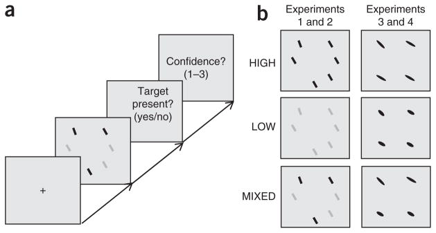
Experimental procedure. (a) Subjects report through a key press whether a predefined target is present in the display, then rate their confidence on a scale from 1 to 3. (b) Experimental conditions. Items in a single display can be all high-reliability (HIGH), all low-reliability (LOW), or a combination of both reliabilities (MIXED). Stimulus reliability was manipulated through contrast in Experiments 1 and 2 (left), and through ellipse eccentricity in Experiments 3 and 4 (right). Example displays show homogeneous distractors; the procedure was identical for heterogeneous distractors.

We examined empirical ROC curves obtained in the LOW and HIGH conditions, along with the best fits of the optimal, single-reliability, and max_x and sum_x models (Fig. 4 and Supplementary Figs. 1–6). The single-reliability model is equivalent to the optimal model in these conditions. From these conditions, we estimated the sensory noise levels associated with a low-reliability and a high- reliability stimulus. Using those two parameters, we predicted the ROCs in the MIXED condition (see Online Methods and Fig. 4). Decision criteria (which incorporate the prior over T) were free parameters. The single-reliability model has an extra parameter, the assumed reliability, which we estimated from the MIXED condition.

Figure 4.

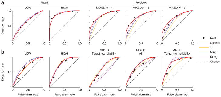
Model predictions for individual-subject receiver operating characteristics. Dots indicate empirical ROC curves. Solid lines show fits (in LOW and HIGH) and predictions (in MIXED) of four models. Stimuli were bars and reliability was manipulated through contrast. (a) Experiment 1 (homogeneous distractors), subject S.N. MIXED trials are grouped by set size. 1r, single-reliability model. (b) Experiment 2 (heterogeneous distractors), subject V.N. MIXED trials are grouped by target reliability. The below-chance ROC curve in the third panel is a result of conditioning on target reliability. Max_d, sum_d, L² and L⁴ model ROC curves are presented as in Supplementary Figures 1–4, along with the ROC curves from other subjects and experiments 3 and 4.

The prediction for the MIXED condition is an important test of the models, as the optimal observer takes into account stimulus reliability (for example, equation (3)) and combines local decision variables in a specific nonlinear manner in this condition (equation (2)). Non-optimal models incorporate only stimulus reliability (max_d, sum_d), the combination rule (single reliability) or neither (max_x, sum_x, L², L⁴). We examined the area under the ROC curve in the MIXED condition (AUC), as measured and as predicted by each model, for each experiment, conditioned on target reliability (Fig. 5 and Supplementary Figs. 7–10). We performed a four-way ANOVA with factors observer type (data or model), stimulus type (bar or ellipse), distractor type (homogeneous or heterogeneous) and target reliability (low or high) on the combined AUC data of all six experiments. On the basis of this analysis, all models besides the optimal model and the max_d model could be ruled out (P < 0.002; Supplementary Results and Supplementary Table 1).

Figure 5.

Model predictions for area under the ROC curve (AUC) in the mixed-reliability condition. For models not shown here, see Supplementary Figures 7 and 10. (a) Data (black), and model predictions obtained from maximum-likelihood estimation in HIGH and LOW (colored lines), in experiments 1 and 3 (homogeneous distractors). Target reliability is high (solid) or low (dashed). (b) Data are presented as in a for experiments 2 and 4 (heterogeneous distractors). Set size was 4 in experiment 2 and 2 in experiment 4. Error bars represent s.e.m. (c) Scatter plot of actual versus predicted AUC for models and individual subjects across all experiments (1 to 4, and auxiliary experiments 1a and 2a; see Supplementary Results). Conditioning on target reliability produces two points per subject.

It is not surprising that summary statistics such as AUC cannot distinguish the optimal model from the max_d model, as the max_d model provides a close approximation to the optimal model. To distinguish between the optimal and the max_d model, we performed Bayesian model comparison on the raw response counts in each response category (Online Methods). This method returns the log likelihood of each model given a single subject’s data; of interest are the differences between the models. We found that the optimal model was the most likely model for all subjects and all experiments. In particular, the log likelihood of the optimal model exceeded that of the max_d model by 25.9 ± 2.2, 8.6 ± 0.8, 5.6 ± 0.6, 56 ± 20, 5.2 ± 0.8 and 60 ± 11 points in experiments 1–4, 1a and 2a, respectively (mean ± s.e.m.). This constitutes decisive evidence that the optimal model better accounts for the data than the max_d model (results across all models and all experiments are shown in Supplementary Table 2, and individual-subject log likelihood differences are shown in Fig. 6 and Supplementary Fig. 9c,d). Taken together, our results indicate that humans perform near-optimal visual search, regardless of whether distractors are homogeneous or heterogeneous and whether the reliability of the stimulus was controlled by contrast or shape.

Figure 6.

Log likelihood of nonoptimal models relative to the optimal model for individual subjects. Subjects are labeled by color, separately for each experiment. Negative numbers indicate that the optimal model fits the human data better.

Neural implementation

Our finding that humans take into account the reliabilities of individual stimuli on a trial-by-trial basis during visual search raises the question of how this is accomplished by neurons. Computing the local decision variable requires knowledge about the reliabilities, $1/{\sigma }_i^2$, on a single trial (for example, equation (3)). How does the nervous system know these reliabilities? Previous models assumed that the only information available to the nervous system at the i^th location is the noisy scalar observation x_i^6,15,19,23, which is sometimes identified with the activity of a single neuron^15,16. Such a coding scheme cannot possibly encode both the orientation of a stimulus and its reliability, as a scalar cannot unambiguously represent two uncorrelated quantities. This is not a problem if reliability is fixed across locations and trials. However, we found that human subjects are near-optimal even in situations in which the reliability of the orientation varies between locations and over time, implying that the neural representation of each stimulus contains information about both orientation and reliability.

Thus, we propose that the brain uses probabilistic population codes^13,25 to encode likelihood functions over orientation on single trials and to compute the posterior probability of target presence. We assume that the orientation at the i^th location is encoded in a population of neurons whose activity we denote by a vector r_i (Fig. 7a). On repeated presentations of the same orientation s_i, the population pattern of activity will vary. We assume that this variability, denoted p(r_i|s_i), belongs to the Poisson-like family of distributions¹³,

Figure 7.

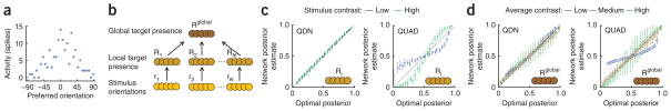
Neural implementation of near-optimal visual search. (a) Example population pattern of activity encoding orientation at one location. Neurons are ordered by their preferred orientation. (b) Network architecture. (c) Posterior probability of local target presence encoded in the second layer versus the optimal posterior probability, when distractors are heterogeneous. Color indicates stimulus contrast. Left, QDN network. Right, QUAD network. Results for other networks and homogeneous distractors are shown in Supplementary Figures 12 and 13. (d) Posterior probability of global target presence encoded in the third layer versus the optimal posterior probability. Left, QDN network. Right, QUAD network. Color indicates the average contrast in the display; across all displays, the histogram of contrasts was binned into low, medium and high. Results for other networks are shown in Supplementary Figure 14. Error bars represent s.d.

$$p({\mathbf{r}}_i\mid s_i,{\mathbf{c}}_i)=\varphi ({\mathbf{r}}_i,{\mathbf{c}}_i)exp({\mathbf{h}}_i(s_s)·{\mathbf{r}}_i)$$ (5)

where ϕ is an arbitrary function and c_i denotes parameters such as local contrast and other image properties, which can affect neural activity and stimulus reliability but are unrelated to our task-relevant feature, orientation. The function h_i(s_i) is related to the tuning curves f_i(s_i,c_i) and the covariance matrix Σ_i(s_i,c_i)¹³ (see Supplementary Fig. 11a). Poisson-like variability is considerably more general than independent Poisson variability while being broadly consistent with the statistics of neuronal responses in vivo.

For a given population activity r_i, we can compute the likelihood function of the stimulus, L(s_i) = p(r_i|s_i), which is proportional to exp(h_i(s_i)·r_i). The value of s_i that maximizes L(s_i), the maximum-likelihood estimate of orientation obtained from r_i, corresponds to the observation x_i described above. The width of the likelihood function, σ_i, indicates the reliability of the orientation information at the i^th location. This automatic encoding of reliability on a single trial might be utilized to build a network that accounts for the near-optimal behavior of the subjects. Such a network would have to implement the marginalizations over distractor orientation (equation (4)) and location (equation (2)) that are required to compute the log likelihood ratios of local and global target presence, respectively.

We trained a three-layer feedforward network (Fig. 7b) using a quadratic nonlinearity^26,27 and divisive normalization^28,29 to perform both marginalizations. The input layer encoded the local orientations using probabilistic population codes, the second layer was trained to compute the log likelihood ratios of local target presence and the third layer was trained to compute the log likelihood ratio of global target presence. The choice of the quadratic nonlinearity and divisive normalization was motivated by our previous finding that these types of operations can be used to implement near- optimal marginalization over discrete probability distributions encoded with probabilistic population codes³⁰. Moreover, with this particular choice of nonlinearities, all layers encode the log likelihood ratio of target presence with probabilistic population codes similar to the ones used in the input layer. These codes have the advantage that the log likelihood ratios of local and global target presence are linearly decodable from the second and third layers (Online Methods), thus simplifying downstream computation and learning.

Networks were trained separately for the homogeneous and heterogeneous cases. We decoded network activity in the second and third layers under the assumption of a Poisson-like probabilistic population code. We expect the network to perform optimally only if this assumption is satisfied, which is to say, if the log likelihood ratio of target presence is linear in the activity of the network units (equation (9)). The network with a quadratic nonlinearity and divisive normalization (QDN) provides a very close approximation to the optimal posterior distribution over local and global target presence (Fig. 7c,d and Supplementary Figs. 12–14). Notably, when we used a network with only a quadratic nonlinearity, but no divisive normalization (QUAD), performance degraded markedly (Fig. 7c,d). The same held for networks without quadratic operations (Supplementary Figs. 12–14). This suggests that divisive normalization is needed to ensure that the log likelihood ratio is approximately linear in the output activity. In Supplementary Figure 15, information loss per layer is compared between the four networks we tested, for both homogeneous and heterogeneous distractors.

Finally, we used the QDN network to generate ROC curves for homogeneous and heterogeneous distractor conditions (Fig. 8). The resulting ROC curves provide accurate fits to the ROC curves obtained from the human subjects. In short, this network, as with our human subjects, is capable of computing a close approximation of the probability of target presence when presented with any arrangement of reliabilities. When neural variability is no longer Poisson-like, the network fails to be near-optimal (Supplementary Fig. 16).

Figure 8.

Neural network reproduces human search performance. ROC curves of the same human observers as in Figure 4 (dots) and the best-fitting QDN network (line). (a) Homogeneous distractors (experiment 1). (b) Heterogeneous distractors (experiment 2).

It is worth noting that with the probabilistic code that we used, input-layer neurons that have the target orientation in a steep region of their tuning curves contribute most to performance (Supplementary Fig. 11b), consistent with earlier theoretical³¹ and experimental studies^32,33 using discrimination tasks but in contrast with the idea that the neuron best tuned to the target orientation is most important¹⁵.

Predictions

Physiological studies have reported neural correlates of decision confidence or certainty in lateral interparietal cortex (LIP)³⁴, superior colliculus³⁵ and orbitofrontal cortex³⁶. Consistent with these findings, our results predict that neurons exist that encode the log likelihood ratio of target presence. The absolute value of the log likelihood ratio is a measure of certainty. Clearly, any model would predict the existence of such neurons given our behavioral data, but our probabilistic population code framework makes a much more specific prediction regarding the mapping from neural activity to probability of target presence. Specifically, an optimized linear decoder of the response of these neurons should be able to recover the log likelihood ratio of global target presence as well as any nonlinear decoder. This is a direct consequence of the fact that in our near-optimal network, neuronal response statistics are constrained to belong to the Poisson-like family in all layers. Moreover, the log likelihood ratio of global target presence should be recoverable with a single linear decoder of neural activity regardless of the reliabilities of target and distractors. These are nontrivial predictions because, in general, nonlinear decoders are expected to perform better than linear decoders. Similarly, a family of linear decoders, each specialized for a particular level of reliability, should, in principle, outperform a single linear decoder. In this case, however, we argue that a nonlinear decoder, or a family of specialized linear decoders, would not extract substantially more information about the posterior distribution than a single linear one. Analogous predictions apply to the log likelihood ratio of local target presence. The prediction that the neural code is optimally linearly decodable in a way that is invariant to the value of nuisance parameters such as contrast has very direct implications for downstream processing, as it simplifies the neural implementation of other probabilistic inferences. For instance, with such a code, the maximum-likelihood estimate can be extracted through attractor dynamics³⁷ and optimal cue integration can be performed through a fixed linear combination of neural activity¹³.

So far, we have not specified where one might expect to find the neurons whose response can be mapped linearly onto the log likelihood ratio of target presence. Although an extensive literature exists on the neural basis of visual search and attention, we are not aware of any studies that have recorded neuronal activity in a single-feature search task with short presentation times and sensory uncertainty. Nevertheless, good candidate regions would be area V4, inferior temporal cortex and LIP, in which strong attentional modulation has been reported. In a multidimensional search task, V4 neurons had a higher response to a target than to a distractor, regardless of the feature dimension in which the target was defined³⁸. The responses of V4 and inferior temporal cortex neurons contain information about which of two stimuli matches a memorized cue³⁹. LIP neurons respond more strongly when an item in their receptive field is a search target than when it is not⁴⁰.

A final prediction concerns the contrast response function of the neurons involved in the marginalization over location when reliability is controlled by contrast. We claim that this marginalization is implemented using a set of basis functions, some of which combine activity from the second layer through quadratic operations with divisive normalization. One can think of these basis functions as neurons in an intermediate layer (between the second and the third) that combine information from multiple locations. Consider a situation in which the set size is 2, that is, two bars appear in the receptive field of such a neuron. The response of this neuron to the contrast of the two bars should follow the quadratic divisive normalization equation. Thus, if the contrast of the second bar is held constant, then the neural response should saturate with increasing contrast of the first bar. Moreover, it should saturate at a level that is monotonically related to the contrast of the second bar. This prediction is task specific: for example, in our previous work on optimal multisensory integration¹³, we predicted that cells combine their multisensory inputs linearly. There, the probabilistic operation needed was a product of distributions, not a marginalization.

DISCUSSION

Searching efficiently for a target amidst distractors is crucial for an organism’s survival. This task is challenging because the reliability of sensory information may vary unpredictably across space and time. Whether and how humans take into account varying reliability in and across displays is an important question from a behavioral, computational and neural perspective. Studies testing the notion of perception as optimal inference have concentrated on simple tasks such as combining cues about a single physical stimulus variable. To take this approach to the next level, it is important to consider perceptual tasks with more complex generative models, such as visual search. As visual search is a task with a hierarchical structure, optimal search requires marginalization, a computation that is ubiquitous in naturalistic visual environments but remains understudied in psychophysics^41,42. We found that human observers take into account reliability on an item-by-item and trial-by-trial basis during visual search and can combine information across locations through marginalization. These results were consistent whether we manipulated the reliability of the items via changes of their contrast or shape. This indicates that human subjects encode probability distributions over stimuli, rather than point estimates, and that they use these distributions to compute the probability of target presence. Human near-optimality in judging an abstract, categorical variable such as target presence provides evidence for the generality of human ability to compute with probability distributions. Exploring complex generative models can contribute to shifting the discourse on optimality in perception toward the question of which task factors might cause performance to be suboptimal. It is likely that greater deviations from optimality will be found in tasks that have more nodes in their generative model or that are less ecologically relevant.

We determined how neural circuits could implement near-optimal visual search using probabilistic population codes and biologically plausible operations, namely a quadratic nonlinearity with divisive normalization. This coding scheme allows a neural network to take into account reliability without requiring a separate circuit to represent this reliability. Moreover, we predict that the interactions implementing near-optimal visual search are different between homogeneous and heterogeneous distractor distributions; in the former, linear neural operations are sufficient to optimally compute local target presence, whereas in the latter, nonlinear operations are needed. We predict that, under both distributions, divisive normalization is an important operation in computing global target presence. This is interesting in light of the proposal that divisive normalization might have a crucial role in the neural basis of attention²⁹. Our results indicate that the same nonlinearity might explain how humans can be near-optimal in the attentional task of searching for a target among distractors. It would be worthwhile to revisit feature-based attention studies from this near-optimality perspective.

Our work is related to previous studies of visual search under sensory noise. An influential study examined eye movements in search scenes corrupted by pixel noise and found that, on average, observers choose their next fixation location according to the maximum probability of identifying the target¹⁷. This work, however, did not address the difficult issue of combining information across spatial locations through marginalization. One of us has previously argued that a saliency-based⁴³ signal-to-noise framework can explain bottom-up and top-down effects on search difficulty in various distractor conditions better than a signal-detection theory model⁴⁴. However, the saliency-based model was not probabilistic and could not easily represent stimulus uncertainty; moreover, the signal detection theory model used was far from optimal. Here the local likelihood ratio of target presence was computed from task-specific probability distributions and can therefore be regarded as a form of top-down saliency. This is similar to a recent model that defined saliency as the posterior probability of local target presence⁴⁵. However, this work considered the scenario of target presence being independent across locations (there can thus be any number of targets) and subsequently focused on feature priors during free viewing. Finally, it has been found that when the distractor distribution is varied between blocks, a max rule applied to local log likelihoods better accounts for human behavior than a maximum-of-outputs rule⁴⁶. This study, however, did not test the optimal rule, equation (2), or vary the reliabilities of the stimuli on a trial-by-trial basis. Changing reliability on a trial-by-trial basis, as we have done, makes the task considerably more difficult, as the reliability of the stimuli must now be taken into account on the fly.

The formalism that we used applies to tasks in which stimulus presentation time is short, at most one target is present and observers report target presence instead of target location. Nonetheless, our framework can be extended to reaction-time procedures by combining it with optimal evidence accumulation⁴⁷, target detection in the presence of multiple targets by replacing the sum in equation (2) by a sum over subsets and target localization by computing the posterior p(T_i = 1|x,T = 1) instead of p(T = 1|x). We hope that our work will facilitate rigorous tests of optimality in a variety of search tasks.

Finally, although we focused on probabilistic population coding, it is quite possible that near-optimal visual search could be implemented with other types of neural codes for probability distributions. Implementing visual search with any scheme is a nontrivial task as it requires tackling the difficult problem of marginalization. Nonetheless, such extensions would be invaluable as they can lead to experimental predictions that would allow us to distinguish between alternative theories of neural coding.

ONLINE METHODS

Experiment 1: manipulating bar contrast, homogeneous distractors

Subjects viewed the display (28 by 21 deg) of dimensions 0.3 by 1.8 deg (the items) on a 21-inch CRT monitor with a refresh rate of 120 Hz and background luminance of 18.8 cd m⁻² from a distance of 85 cm. Target and distractor orientations were −70° and −60°, respectively. Items were displayed in one of eight possible positions (corresponding to compass directions), equally spaced around an imaginary circle of radius 7 deg, centered at a central fixation cross. Item positions were randomly chosen for set sizes 4 or 6. Each item position had a uniform random jitter of up to 0.6 deg in both x and y directions. Item contrast was either 67% (high) or 12 or 17% (low), according to the subject.

In the LOW and HIGH conditions, set size was 8 and all items had the same contrast (low or high, respectively). In the MIXED condition, set size was 4, 6 or 8 (intermixed in pseudorandom order) and the contrast of each item was randomly and independently set to high or low. On each trial, the probability that the display contained a target was 0.5; subjects were informed of this in advance. If the target was present, its location was chosen randomly.

Each trial began with fixation (250 ms), followed by the search display, followed by a blank screen until the subject responded. Subjects gave a yes/no response about target presence, followed by a confidence rating on a scale of 1 to 3 (1 = least confident, 3 = most confident). Subjects were encouraged to spread their responses across the ratings. Subjects practiced for 30 trials in the HIGH conditions with a 200-ms stimulus, and they received correctness feedback at the end of each trial. After practice, subjects performed a variable number of 30-trial blocks in the HIGH condition starting with a 200-ms stimulus. Stimulus duration decreased by 25 ms on every subsequent block, until accuracy was 85–90%. The resulting stimulus durations of 50 or 75 ms were subsequently used throughout the experiment. Subjects then performed two 120-trial blocks in the HIGH condition with 67% contrast items. Next, stimulus contrast (identical for all items in a display) decreased in 30-trial blocks by 5% on every subsequent block until accuracy reached was 60 to 65%. The resulting contrast was used as low contrast. The subject then performed two 120-trial blocks in the low condition, followed by practice on 30 trials in the mixed condition (without feedback) and six 120-trial blocks in the mixed condition.

The experiments were conducted over two sessions on consecutive days. All stimuli were controlled using MATLAB (MathWorks) with the Psychophysics Toolbox⁴⁸. Four subjects (two authors, two naive) participated. Informed written consent was obtained from all subjects.

Experiment 2: manipulating bar contrast, heterogeneous distractors

This experiment was identical to Experiment 1, except for the following differences. Set size was 4 and target orientation was −60°. Distractor orientation was randomly sampled from all multiples of 9° away from the target. Stimuli were placed at every other possible location from Experiment 1, starting at northeast. Each subject performed two 120-trial blocks in the LOW (L), HIGH (H) and MIXED (M) conditions, in the order HHLLMM. High and low contrasts were 61% and 16%, respectively. Four subjects (one author, three naive) participated.

Experiments 3 and 4: manipulating ellipse eccentricity

Experiments 3 and 4 were identical to experiments 1 and 2, except for the following differences. Subjects viewed the display on a 19-inch LCD monitor with a refresh rate of 60 Hz and background luminance of 34 cd m⁻², from a distance of 60 cm. Items were ellipses; ellipse orientation was defined by the orientation of the long axis. The area of each ellipse was 0.24 deg² and reliability was manipulated through ellipse eccentricity (elongation). Target orientation was −45°. In experiment 3, distractors were homogeneous with an orientation chosen per subject (−30°, −25°, −15°) to ensure that asymptotic accuracy at high eccentricity exceeded 87.5%. In experiment 4, distractors were heterogeneous and drawn from a uniform distribution. The set size was 2 or 4 (separate sessions) in experiment 3 and 2 in experiment 4. When the set size was 2, stimuli were placed at the northwest and southeast locations. When the set size was 4, stimuli were placed at these locations and also at northeast and southwest. Stimulus duration was 300 ms during practice and 66.7 ms during testing.

Subjects performed three types of blocks: practice, threshold measurement and testing. During practice, stimulus duration was 300 ms, stimuli were of mixed reliability, subjects did not report confidence, trial-to-trial correctness feedback was given by briefly coloring the fixation cross green or red and an image of the target with eccentricity 0.9 was displayed at the location of the fixation cross for 500 ms before the start of a new trial. During threshold measurement blocks, a psychometric curve (percentage correct versus ellipse eccentricity) was mapped out to determine 62.5% and 87.5% thresholds at N = 4 (experiment 3) or N = 2 (experiment 4). These eccentricities provided the low and high values of eccentricity throughout the experiment. In experiment 3, (low, high) eccentricity pairs were (0.66, 0.82) for subject R.B., (0.65, 0.92) for subject W.M. and (0.61, 0.78) for subject E.A. In experiment 4, they were (0.50, 0.82) for subject R.B., (0.56, 0.93) for subject W.M. and (0.47, 0.90) for subject E.A. Experiment 3 consisted of three sessions. In the first session (N = 4), subjects performed a 100-trial practice block, two 150-trial threshold measurement blocks and three 150-trial testing blocks in the order HML. In the second session (N = 4), subjects performed a 100-trial practice block and five 150-trial testing blocks in the order MMLMH. In the third session (N = 2), subjects performed a 100-trial practice block, followed by four 150-trial blocks in the mixed condition. Experiment 4 consisted of two sessions, organized in the same way as the first two sessions of experiment 3. The same three subjects (two authors, one naive) participated in experiments 3 and 4.

Experiments 1a and 2a: manipulating bar contrast at N = 2

Experiments 1a (homogeneous distractors) and 2a (heterogeneous distractors) were identical to experiments 1 and 2, respectively, except for the following differences. Set size was always 2. Three subjects (two of them authors) participated in both experiments. Background luminance was 95 cd m⁻². Each item was an oriented bar of dimensions 0.3 by 0.8 deg. Target orientation was −45° and distractor orientation was −35° for RB and −30° for subjects W.M. and S.K. These values were chosen to ensure that for each subject, asymptotic accuracy at high contrast exceeded 87.5%. The procedure consisted of practice, threshold measurement and testing and was analogous to that of experiment 4. During threshold measurement, a psychometric curve was mapped out to determine 62.5% and 87.5% thresholds. These contrasts provided the low and high values of reliability throughout the experiment. In experiment 1a, these pairs were (5.6%, 20%) for subject R.B., (3.8%, 7.8%) for subject S.K. and (4%, 11%) for subject W.M. In experiment 2a, they were (4.8%, 14%) for subject R.B., (2.9%, 9.6%) for subject S.K. and (4%, 12%) for subject W.M. Stimulus duration was 300 ms during practice and 33 ms during threshold measurement and testing.

Model predictions

An experimental condition is a combination of target presence, set size and reliability condition (LOW, MIXED, HIGH). Generating model predictions for each condition consisted of choosing parameter values, simulating observations for 100,000 trials using those parameters and letting the model make decisions on the simulated observations.

In experiments 1 and 3, the model parameters (denoted θ), were σ_low, σ_high and five decision criteria (in all models), as well as σ_assumed (in the single-reliability model). Internal representations x_i were drawn independently from normal distributions with identical variances, ${\sigma }_i^2$, and means of 10° (target) and 0° (distractor). Here, σ_i is either σ_low or σ_high. In experiments 2 and 4, the internal representation of a stimulus was drawn from a Von Mises distribution centered at the stimulus orientation and with concentration parameter κ_i (either κ_low or κ_high). In the max_x, sum_x, L² and L⁴ models, the local decision variable was taken to be the output of a Poisson neuron with a Von Mises tuning curve that responded most strongly to the target orientation: r_i = Poisson(g_i exp(κ_tc cos(2(s – s_T))) + b), where g_i is either g_low or g_high (see Supplementary Results). We chose κ_tc = 1.5 and b = 5 and verified that our results were insensitive to this choice of parameters. This suboptimal local decision variable is consistent with earlier proposals^15,16 and, unlike x_i, respects the circularity of orientation space. On each simulated trial, a given model infers whether the target is present by computing a global decision variable d from local decision variables {d_i}, and those in turn from the observations {x_i} or {r_i}. The local decision variable of the optimal, single-reliability, max_d and sum_d models in experiments 2 and 4 is given by d_i= −log I₀(κ_i) + κ_icos(2(x_i - s_T)), where I₀ is the modified Bessel function of the first kind of order 0 (see Supplementary Results). In the same four models, the value of the parameter σ_i (or g_i or κ_i) used in the decision variable equals the value used in the generative model (for example, σ_low or σ_high), except in the MIXED condition of the single-reliability model, in which each σ_i (or κ_i) is equal to σ_assumed (or κ_assumed). All models contain σ_low and σ_high (or κ_low and κ_high) as free parameters, although the decision variables of some models (single reliability, max_x, sum_x, L², L⁴) do not contain those parameters, as these parameters determine the distributions of observations and are therefore necessary in the step of simulating those. Once d has been computed for all trials, we can plot its distribution in target-present and target-absent displays, p(d | T = 1) and p(d | T = 0), as we did in Figure 2a. We obtained model ROC curves by varying the decision criterion τ along the real line and plotting the resulting hit rates, p(d > τ|T = 1), and false-alarm rates, p(d > τ | T = 0), against each other, as in Figure 2b.

Comparing the value of d on each trial against the five criteria yielded predictions for response frequencies. The criteria between which d lies on a given trial determines which of the six possible responses R (target presence judgment × confidence rating) the model makes. The result is a set of predicted frequencies for a given model, given model parameters and experimental condition C; we denote these by p(R | model,θ,C).

Prediction analysis

For each model, we computed the probability of a subject’s data given a set of hypothesized parameter values θ, p(data | model,θ). The data on the i^th trial, data_i, consist of the experimental condition C and the subject’s response R. We assume that the data on different trials are independent when conditioned on model and parameters. We can then factorize p(data | model,θ) by organizing the trials by condition C and subject response R

$$\begin{array}{l}p(\text{data}\mid \text{model},\mathbf{\theta })=\prod _{i}p({\text{data}}_i\mid \text{model},\mathbf{\theta })\\ =\prod _C\prod _{R=1}^6\prod _{\begin{array}{c}\text{trials}i\\ \text{with}C\text{and}R\end{array}}p(R\mid \text{model},\mathbf{\theta },C)\\ =\prod _C\prod _{R=1}^{6}p{(R\mid \text{model},\mathbf{\theta },C)}^{n_R(C)},\end{array}$$ (6)

where n_R(C) is the number of trials in condition C on which the subject responded R. Equation (6) is conveniently expressed as a log probability

$$logp(\text{data}\mid \text{model},\mathbf{\theta })=\sum _C\sum _{R=1}^6{n}_R(C)logp(R\mid \text{model},\mathbf{\theta },C)$$ (7)

This is an inner product between the observed response counts and the predicted log probabilities. For given model, condition and reliability parameter values, possible values of each criterion ranged from the smallest to the largest value of the simulated decision variable in 30 equally spaced steps. After computing the likelihood p(data | model, θ) of each parameter combination θ, we numerically marginalized over all five criteria. In experiments 1 and 3, this resulted in a likelihood p(data | model, σ_low) for the LOW and p(data | model, σ_high) for the HIGH condition. We fitted non-normalized Gaussians to these parameter likelihoods to reduce the effects of sampling noise and used their modes as estimates of σ_low and σ_high. We used these estimates to plot the fitted LOW and HIGH ROC curves, as well as to predict the MIXED ROCs from the model. The analysis for experiments 2 and 4 was identical, but with each σ replaced by a κ or g. In all experiments, the single-reliability model has an extra parameter, σ_assumed or κ_assumed; we estimated its value from the N = 4 trials in the MIXED condition in experiments 1 and 3, and from all trials in the MIXED condition in experiments 2, 4, 1a and 2a.

ROC curves

Cumulative summation of responses across the six response categories yielded empirical ROC curves. For ROC curves conditioned on target reliability, we used the conditioned target-present trials and all of the target-absent trials. We approximated the area under the ROC curve by summing the areas of the six trapezoids formed by pairs of neighboring ROC points and the x axis. The area under a model ROC curve was computed from the trapezoids based on the six model points with false alarm rates closest to the false alarm rates in the data.

Bayesian model comparison

We computed the likelihood of each model by marginalizing over model parameters θ

$$p(\text{data}\mid \text{model})=\int p(\text{data}\mid \text{model},\mathbf{\theta })p(\mathbf{\theta }\mid \text{model})d\mathbf{\theta }$$ (8)

This method utilizes the full statistical power of the data and allows for a fair comparison between models with different numbers of parameters⁴⁹. The first factor in the integrand is computed from equation (7). For the prior over parameters, p(θ | model), we chose a uniform distribution on a reasonable range chosen in advance. Our model comparison results were not sensitive to the choice of this range. We approximated the integral by a Riemann sum and compared the resulting number across models.

Neural implementation

Computing the local and global log likelihood ratios of target presence requires marginalization: the former over distractor orientation (when distractors are heterogeneous) and the latter over target location. We sought a neural network model that performs both marginalizations near optimally, while simultaneously encoding both T_i and T are in Poisson-like probabilistic population codes. We assumed reliability is manipulated through contrast.

Our first aim was to find a mapping, R_i = F(r_i), from a Poisson-like input pattern of population activity encoding orientation, r_i, to a Poisson-like output population R_i that optimally encodes local target presence, T_i. This is accomplished when the approximate posterior, q(T_i | R_i = F(r_i)), is close to the optimal posterior computed from the inputs, p(T_i | r_i), for each input pattern of activity r_i. As we desired a Poisson-like population code in the output, we assumed q(T_i | R_i) to satisfy

$$\begin{array}{l}q(T_i=1\mid {\mathbf{R}}_i)=\frac{e^{{\mathbf{H}}_i(T_i=1)·{\mathbf{R}}_i}}{e^{{\mathbf{H}}_i(T_i=0)·{\mathbf{R}}_i}+e^{{\mathbf{H}}_i(T_i=1)·{\mathbf{R}}_i}}=\frac{1}{1+e^{-({\mathbf{H}}_i(T_i=1)v-{\mathbf{H}}_i(T_i=0))·{\mathbf{R}}_i}}\\ =\lambda (\mathbf{\Delta }{\mathbf{H}}_i·{\mathbf{R}}_i)\end{array}$$ (9)

where λ(x) = 1/(1+exp(−x)) is the logistic function and ΔH_i = H_i(T_i = 1) − H_i(T_i = 0). Here H_i(T_i) is the kernel belonging to T_i, in analogy to h_i(s_i), which was the orientation-dependent kernel in the input layer. By rewriting equation (9) as

$$log\frac{q(T_i=1\mid {\mathbf{R}}_i)}{q(T_i=0\mid {\mathbf{R}}_i)}=\mathbf{\Delta }{\mathbf{H}}_i·{\mathbf{R}}_i$$

we see that Poisson-like variability in the output implies that the log likelihood ratio of local target presence is linearly decodable from neural activity, R_i (the same holds for global target presence). When distractors are homogeneous, we can simply choose R_i = r_i, H_i(T_i = 1) = h_i(s_T), and H_i(T_i = 0) = h_i(s_D); that is, the input layer already forms a Poisson-like probabilistic population code for local target presence. However, with heterogeneous distractors, the neural operations between the first and the second layer need to implement marginalization over distractor orientation.

This marginalization constitutes a transformation of the population pattern of activity r_i, which represents the probability distribution over the stimulus at the i^th location, into a new pattern of activity R_i that represents the probability distribution over local target presence, T_i. Even if H_i were known, the approximation problem of finding R_i in terms of r_i is underconstrained, as a large family of functions of r_i can yield the same posterior q(T_i | R_i). To constrain this problem, we only used operations, F(r_i), that are neurally plausible and useful in other probabilistic computations. The operations that we considered were linear, quadratic and divisive normalization. We tested four networks, defined by the following basis sets of operations (the location index i of the population is left out here to avoid clutter; the indices j and k refer to neurons)

$$\begin{array}{l}{\mathbf{z}}^{\text{LIN}}=\{1,r_j\}\\ {\mathbf{z}}^{\text{QUAD}}=\{1,r_j,r_j{r}_k\}\\ {\mathbf{z}}^{\text{LDN}}=\left\{1,r_j,\frac{1}{a_0+{\displaystyle \sum _k}{a}_k{r}_k},\frac{r_j}{a_0+{\displaystyle \sum _k}{a}_k{r}_k}\right\}\\ {\mathbf{z}}^{\text{QDN}}=\left\{1,r_j,\frac{1}{a_0+{\displaystyle \sum _k}{a}_k{r}_k},\frac{r_j}{a_0+{\displaystyle \sum _k}{a}_k{r}_k},\frac{r_j{r}_k}{a_0+{\displaystyle \sum _k}{a}_k{r}_k}\right\}\end{array}$$

All a_i are constants. We call these networks linear (LIN), quadratic (QUAD), linear plus divisive normalization (LDN) and quadratic plus divisive normalization (QDN). The j^th element of R_i is now a linear combination of the elements of the basis set, with weights w_i = [w_ijk]

$$R_{ij}=\sum _k{w}_{\mathit{ijk}}{z}_{ik}$$

The approximate posterior for a given network is then

$$q(T_i=1\mid {\mathbf{z}}_i,{\mathbf{W}}_i)=\lambda \left(\sum _{j,k}\mathrm{\Delta }{H}_{ij}{w}_{\mathit{ijk}}{z}_{ik}\right)=\lambda \left(\sum _k{w}_{ik}{z}_{ik}\right)=\lambda ({\mathbf{w}}_i·{\mathbf{z}}_i)$$ (10)

where w_ik = Σ_j ΔH_ijw_ijk and w_i = [w_ik]. Thus, the weight matrix w_i and the output kernel vector ΔH_i are combined into a single vector of unknown weights. Finding w_i in equation (10) is a logistic regression problem, which we treated by applying stochastic gradient descent to the Kullback-Leibler divergence between the optimal posterior and the approximate posterior from the network. Kullback-Leibler divergence is a principled measure of the distance between two probability distributions⁵⁰. Its trial average (at fixed gain) can be expressed as follows

$${\langle D_{\text{KL}}\left(p\left(T_i\mid {\mathbf{r}}_i,g_i\right)\Vert q\left(T_i\mid {\mathbf{z}}_i\left({\mathbf{r}}_i\right)\right)\right)\rangle }_{{\mathbf{r}}_i}={\langle logp\left(T_i\mid {\mathbf{r}}_i,g_i\right)-logq\left(T_i\mid {\mathbf{z}}_i\left({\mathbf{r}}_i\right)\right)\rangle }_{T_i,{\mathbf{r}}_i}$$ (11)

where the braces denote an expectation over the joint distribution p(T_i,r_i | g_i). We approximated this average by sampling from the generative model. We first randomly drew pairs of data (T_i, s_i) according to the task statistics. Having obtained s_i, a pattern of activity r_i was obtained by sampling from a Poisson-distributed population of 20 neurons with preferred orientations {s̄_ij}, equally spaced on the interval [0,π). The tuning curve of the j^th neuron was given by $f_{ij}\left(s_i,c_i\right)=g_i\left(c_i\right)exp\left({\kappa }_{\text{tc}}\left(cos2\left(s_i-{\overline{s}}_{ij}\right)-1\right)\right)$, where κ_tc = 2, c_i is contrast, and gain g_i was randomly set to 0.5 for a low-contrast item or to 3 for a high-contrast item (it is important that each training set contains trials of both gains). This ensured that overall task performance ranged from around 60% correct in the low condition to 85% correct in the high condition. From these activity samples r_i, we obtained basis set samples z_i, calculated the network posteriors q(T_i | z_i) and estimated the gradient of the average Kullback-Leibler divergence. At each gradient step, we generated 10,000 novel samples of r_i. Both the linear weights w_i and the weights of the divisive normalization were learned in this way. A new set of 10,000 activity samples was drawn to calculate each gradient step. Gradient descent was iterated until convergence. We verified convergence of the linear weights by comparing the outcome with the posterior obtained through variational Bayesian logistic regression applied to a novel set of samples.

At the completion of the learning phase, an additional 10,000 samples were generated at both gains, and network estimates of the posterior over T_i were computed using the learned weights. We plotted the estimated posteriors against the optimal posteriors in Figure 7c,d and Supplementary Figures 12 and 13. We obtained the proportion information loss by dividing the average Kullback-Leibler divergence between estimated and optimal posterior (equation (11)) by the mutual information between T_i and the input activity, r_i, defined as $I\left(T_i,{\mathbf{r}}_i;g_i\right)={\langle logp\left(T_i\mid {\mathbf{r}}_i,g_i\right)-logp\left(T_i\right)\rangle }_{T_i,{\mathbf{r}}_i}^{T_i}$ (note that this proportion can exceed 1). Mutual information was computed through an average over samples, just like average Kullback-Leibler divergence.

This procedure was repeated for the second marginalization, using as input an optimal Poisson-like population code for local target presence. Marginalization over target location requires a network which transforms N population patterns of activity R₁,…,R_N into a population code R^global which encodes the global log likelihood ratio, d. Thus, there are N gain parameters, rather than just one, as in the first marginalization. Gain was chosen independently for each location, with g_i = 24 and g_i = 4 each selected with probability 0.5. At the i^th location, a population code for local target presence was generated by sampling activity from ten independent Poisson neurons (j = 1,…,10) with means conditioned on $T_i:f_{ij}(T_i,g_i)=g_{i}exp\left({\kappa }_{\text{tc}}\left(cos2\left(\frac{\pi }{18}{T}_i-{\overline{T}}_{ij}\right)-1\right)\right)$. In these (arbitrary) ‘tuning curves’ over T_i, we chose κ_tc = 2, and the set of {T̄_ij} were equally spaced on the interval [0, π). The same four networks were tested as for the first marginalization but with r_i replaced by R. Network ROC curves (Fig. 8) were obtained from the population in the third layer.

References

- 1.Palmer J, Ames CT, Lindsey DT. Measuring the effect of attention on simple visual search. J Exp Psychol Hum Percept Perform. 1993;19:108–130. doi: 10.1037//0096-1523.19.1.108. [DOI] [PubMed] [Google Scholar]
- 2.Treisman AM, Gelade G. A feature-integration theory of attention. Cognit Psychol. 1980;12:97–136. doi: 10.1016/0010-0285(80)90005-5. [DOI] [PubMed] [Google Scholar]
- 3.Estes WD, Taylor RM. A detection method and probabilistic models for assessing information processing from brief visual displays. Proc Natl Acad Sci USA. 1964;52:446–454. doi: 10.1073/pnas.52.2.446. [DOI] [PMC free article] [PubMed] [Google Scholar]
- 4.Shaw ML. Identifying attentional and decision-making components in information processing. In: Nickerson RS, editor. Attention and Performance. Erlbaum; Hillsdale, New Jersey: 1980. pp. 277–296. [Google Scholar]
- 5.Teichner WH, Krebs MJ. Visual search for simple targets. Psychol Bull. 1974;81:15–28. doi: 10.1037/h0035449. [DOI] [PubMed] [Google Scholar]
- 6.Palmer J, Verghese P, Pavel M. The psychophysics of visual search. Vision Res. 2000;40:1227–1268. doi: 10.1016/s0042-6989(99)00244-8. [DOI] [PubMed] [Google Scholar]
- 7.Duncan J, Humphreys GW. Visual search and stimulus similarity. Psychol Rev. 1989;96:433–458. doi: 10.1037/0033-295x.96.3.433. [DOI] [PubMed] [Google Scholar]
- 8.Rosenholtz R. Visual search for orientation among heterogeneous distractors: experimental results and implications for signal detection theory models of search. J Exp Psychol Hum Percept Perform. 2001;27:985–999. doi: 10.1037//0096-1523.27.4.985. [DOI] [PubMed] [Google Scholar]
- 9.Eriksen CW. Object location in a complex perceptual field. J Exp Psychol. 1953;45:126–132. doi: 10.1037/h0058018. [DOI] [PubMed] [Google Scholar]
- 10.Farmer EW, Taylor RM. Visual search through color displays: effects of target-background similarity and background uniformity. Percept Psychophys. 1980;27:267–272. doi: 10.3758/bf03204265. [DOI] [PubMed] [Google Scholar]
- 11.Knill DC, Richards W. Perception as Bayesian Inference. Cambridge University Press; New York: 1996. [Google Scholar]
- 12.Knill DC, Pouget A. The Bayesian brain: the role of uncertainty in neural coding and computation. Trends Neurosci. 2004;27:712–719. doi: 10.1016/j.tins.2004.10.007. [DOI] [PubMed] [Google Scholar]
- 13.Ma WJ, Beck JM, Latham PE, Pouget A. Bayesian inference with probabilistic population codes. Nat Neurosci. 2006;9:1432–1438. doi: 10.1038/nn1790. [DOI] [PubMed] [Google Scholar]
- 14.Morgan ML, DeAngelis GC, Angelaki DE. Multisensory integration in macaque visual cortex depends on cue reliability. Neuron. 2008;59:662–673. doi: 10.1016/j.neuron.2008.06.024. [DOI] [PMC free article] [PubMed] [Google Scholar]
- 15.Verghese P. Visual search and attention: a signal detection theory approach. Neuron. 2001;31:523–535. doi: 10.1016/s0896-6273(01)00392-0. [DOI] [PubMed] [Google Scholar]
- 16.Eckstein MP, Peterson MF, Pham BT, Droll JA. Statistical decision theory to relate neurons to behavior in the study of covert visual attention. Vision Res. 2009;49:1097–1128. doi: 10.1016/j.visres.2008.12.008. [DOI] [PubMed] [Google Scholar]
- 17.Najemnik J, Geisler WS. Optimal eye movement strategies in visual search. Nature. 2005;434:387–391. doi: 10.1038/nature03390. [DOI] [PubMed] [Google Scholar]
- 18.Eckstein MP, Thomas JP, Palmer J, Shimozaki SS. A signal detection model predicts the effects of set size on visual search accuracy for feature, conjunction, triple conjunction, and disjunction displays. Percept Psychophys. 2000;62:425–451. doi: 10.3758/bf03212096. [DOI] [PubMed] [Google Scholar]
- 19.Green DM, Swets JA. Signal Detection Theory and Psychophysics. John Wiley & Sons; Los Altos, California: 1966. [Google Scholar]
- 20.Peterson WW, Birdsall TG, Fox WC. The theory of signal detectability. IRE Prof Group Inf Theory. 1954;4:171–212. [Google Scholar]
- 21.Nolte LW, Jaarsma D. More on the detection of one of M orthogonal signals. J Acoust Soc Am. 1967;41:497–505. [Google Scholar]
- 22.Eckstein MP. The lower visual search efficiency for conjunctions is due to noise and not serial attentional processing. Psychol Sci. 1998;9:111–118. [Google Scholar]
- 23.Graham N, Kramer P, Yager D. Signal dection models for multidimensional stimuli: probability distributions and combination rules. J Math Psychol. 1987;31:366–409. [Google Scholar]
- 24.Quick RF. A vector-magnitude model of contrast detection. Kybernetik. 1974;16:65–67. doi: 10.1007/BF00271628. [DOI] [PubMed] [Google Scholar]
- 25.Pouget A, Dayan P, Zemel RS. Inference and Computation with Population Codes. Annu Rev Neurosci. 2003;26:381–410. doi: 10.1146/annurev.neuro.26.041002.131112. [DOI] [PubMed] [Google Scholar]
- 26.Bremmer F, Ilg U, Thiele A, Distler C, Hoffman K. Eye position effects in monkey cortex. I. Visual and pursuit-related activity in extrastriate areas MT and MST. J Neurophysiol. 1997;77:944–961. doi: 10.1152/jn.1997.77.2.944. [DOI] [PubMed] [Google Scholar]
- 27.Andersen RA, Essick G, Siegel R. Encoding of spatial location by posterior parietal neurons. Science. 1985;230:456–458. doi: 10.1126/science.4048942. [DOI] [PubMed] [Google Scholar]
- 28.Heeger DJ. Normalization of cell responses in cat striate cortex. Vis Neurosci. 1992;9:181–197. doi: 10.1017/s0952523800009640. [DOI] [PubMed] [Google Scholar]
- 29.Reynolds JH, Heeger DJ. The normalization model of attention. Neuron. 2009;61:168–185. doi: 10.1016/j.neuron.2009.01.002. [DOI] [PMC free article] [PubMed] [Google Scholar]
- 30.Beck J, Latham P, Pouget A. Complex Bayesian inference in neural circuits using divisive normalization. Front Syst Neurosci Conference Abstract: Computational and Systems Neuroscience; 2 February, 2009.2009. [DOI] [Google Scholar]
- 31.Seung HS, Sompolinsky H. Simple model for reading neuronal population codes. Proc Natl Acad Sci USA. 1993;90:10749–10753. doi: 10.1073/pnas.90.22.10749. [DOI] [PMC free article] [PubMed] [Google Scholar]
- 32.Schoups A, Vogels R, Qian N, Orban G. Practising orientation identification improves orientation coding in V1 neurons. Nature. 2001;412:549–553. doi: 10.1038/35087601. [DOI] [PubMed] [Google Scholar]
- 33.Regan D, Beverley KI. Spatial–frequency discrimination and detection: comparison of postadaptation thresholds. J Opt Soc Am. 1983;73:1684–1690. doi: 10.1364/josa.73.001684. [DOI] [PubMed] [Google Scholar]
- 34.Kiani R, Shadlen MN. Representation of confidence associated with a decision by neurons in the parietal cortex. Science. 2009;324:759–764. doi: 10.1126/science.1169405. [DOI] [PMC free article] [PubMed] [Google Scholar]
- 35.Kim B, Basso MA. Saccade target selection in the superior colliculus: a signal detection theory approach. J Neurosci. 2008;28:2991–3007. doi: 10.1523/JNEUROSCI.5424-07.2008. [DOI] [PMC free article] [PubMed] [Google Scholar]
- 36.Kepecs A, Uchida N, Zariwala HA, Mainen ZF. Neural correlates, computation and behavioural impact of decision confidence. Nature. 2008;455:227–231. doi: 10.1038/nature07200. [DOI] [PubMed] [Google Scholar]
- 37.Deneve S, Latham P, Pouget A. Reading population codes: a neural implementation of ideal observers. Nat Neurosci. 1999;2:740–745. doi: 10.1038/11205. [DOI] [PubMed] [Google Scholar]
- 38.Ogawa T, Komatsu H. Target selection in area V4 during a multidimensional visual search task. J Neurosci. 2004;24:6371–6382. doi: 10.1523/JNEUROSCI.0569-04.2004. [DOI] [PMC free article] [PubMed] [Google Scholar]
- 39.Bichot NP, Rossi AF, Desimone R. Parallel and serial neural mechanisms for visual search in macaque area V4. Science. 2005;308:529–534. doi: 10.1126/science.1109676. [DOI] [PubMed] [Google Scholar]
- 40.Gottlieb JP, Kusunoki M, Goldberg M. The representation of visual salience in monkey parietal cortex. Nature. 1998;391:481–484. doi: 10.1038/35135. [DOI] [PubMed] [Google Scholar]
- 41.Knill DC. Mixture models and the probabilistic structure of depth cues. Vision Res. 2003;43:831–854. doi: 10.1016/s0042-6989(03)00003-8. [DOI] [PubMed] [Google Scholar]
- 42.Kersten D, Mamassian P, Yuille A. Object perception as Bayesian inference. Annu Rev Psychol. 2004;55:271–304. doi: 10.1146/annurev.psych.55.090902.142005. [DOI] [PubMed] [Google Scholar]
- 43.Itti L, Koch C. Computational modeling of visual attention. Nat Rev Neurosci. 2001;2:194–203. doi: 10.1038/35058500. [DOI] [PubMed] [Google Scholar]
- 44.Navalpakkam V, Itti L. Search goal tunes visual features optimally. Neuron. 2007;53:605–617. doi: 10.1016/j.neuron.2007.01.018. [DOI] [PubMed] [Google Scholar]
- 45.Zhang L, Tong MH, Marks TK, Shan H, Cottrell GW. SUN: a Bayesian framework for saliency using natural statistics. J Vis. 2008;8:1–20. doi: 10.1167/8.7.32. [DOI] [PMC free article] [PubMed] [Google Scholar]
- 46.Vincent BT, Baddeley RJ, Troscianko T, Gilchrist ID. Optimal feature integration in visual search. J Vis. 2009;9:1–11. doi: 10.1167/9.5.15. [DOI] [PubMed] [Google Scholar]
- 47.Beck JM, et al. Bayesian decision-making with probabilistic population codes. Neuron. 2008;60:1142–1152. doi: 10.1016/j.neuron.2008.09.021. [DOI] [PMC free article] [PubMed] [Google Scholar]
- 48.Brainard DH. The Psychophysics Toolbox. Spat Vis. 1997;10:433–436. [PubMed] [Google Scholar]
- 49.MacKay DJ. Information Theory, Inference and Learning Algorithms. Cambridge University Press; Cambridge, UK: 2003. [Google Scholar]
- 50.Cover TM, Thomas JA. Elements of Information Theory. John Wiley & Sons; New York: 1991. [Google Scholar]
Associated Data
This section collects any data citations, data availability statements, or supplementary materials included in this article.