Accurate assessment of mass, models and resolution by small-angle scattering

Abstract

Modern small angle scattering (SAS) experiments with X-rays or neutrons provide a comprehensive, resolution-limited observation of the thermodynamic state. However, methods for evaluating mass and validating SAS based models and resolution have been inadequate. Here, we define the volume-of-correlation, V_c: a SAS invariant derived from the scattered intensities that is specific to the structural state of the particle, yet independent of concentration and the requirements of a compact, folded particle. We show V_c defines a ratio, Qr, that determines the molecular mass of proteins or RNA ranging from 10 to 1,000 kDa. Furthermore, we propose a statistically robust method for assessing model-data agreements (X²_free) akin to cross-validation. Our approach prevents over-fitting of the SAS data and can be used with a newly defined metric, R_sas, for quantitative evaluation of resolution. Together, these metrics (V_c, Qr, X²_free, and R_sas) provide analytical tools for unbiased and accurate macromolecular structural characterizations in solution.

Achieving reliable, high-throughput structural characterizations of biological macromolecular complexes is a major challenge in the modern structural-genomics era¹. In principle, small-angle scattering (SAS) with X-rays (SAXS) or neutrons (SANS) can meet this challenge by efficiently providing information that fully describes the structural state of a macromolecule in solution^2–4. SAS can determine a scattering particle’s radius-of-gyration (R_g), volume (V_p), surface-to-volume ratio and correlation length (l_c) with the latter three physical parameters dependent on the Porod invariant⁵, Q, an empirical SAS value defined for compact folded particles. Q is unique to a scattering experiment and requires convergence of the SAS data at high scattering vectors (q, Å⁻¹) in a q²⋅I(q) vs. q (Kratky) plot. Convergence defines an enclosed area where the degree of convergence reflects the compacted (bounded area), flexible, or unfolded (unbounded area) solution states (Fig. 1a). Consequently, non-convergence leaves Q undetermined and paradoxically implies V_p and l_c are undefined for flexible particles (SI Fig. 1 and Notes). This observation leaves R_g as the only structural parameter that can be reliably derived from SAS data on flexible systems.

Figure 1. Concentration independence and conformational dependence of V_c.

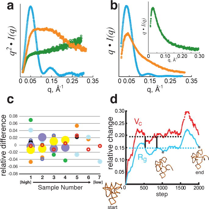
(a, b), Experimental SAXS data plotted on a relative scale for glucose isomerase (cyan), 94-nucleotide SAM-1 riboswitch in the absence of Mg²⁺ (orange) and RAD51AP1, an intrinsically unfolded protein (green). a, Data transformed as the Kratky plot, q²• I(q) vs. q, reveal the parabolic convergence for a folded particle (blue) and divergence for a flexible (orange) or fully unfolded (green) particle. b, Data plotted as q • I(q) vs. q show convergence for both folded and flexible particles. Inset demonstrates convergence for a fully unfolded polymer. c, Concentration independence of V_c for experimental SAXS data. For each of 7 samples, relative difference is calculated as the deviation from the mean normalized to the mean. Concentrations ranged from 0.2 to 3 mg/mL for glucose isomerase (cyan), P4–P6 domain (open red), xylanase (orange), TyMV UUAG TLS RNA (solid black), del8 RNA (open purple), Atu RNase P(open black), SAM-1 riboswitch with Mg²⁺ and ligand (closed purple), SAM-1 riboswitch in the absence of Mg²⁺ (solid green). X-axis (Sample Number) refers to the different concentrations for each sample increasing from left to right. d, Correlated changes in V_c (red) and R_g (cyan) for conformations of SAM-1 riboswitch (PDB 2GIS) simulated from molecular dynamics with CNS²⁸. Horizontal lines demonstrate for R_g or V_c that a single value can map to multiple conformations. Dual specification of both R_g and V_c reduces multiplicity (vertical bars). Relative change represents the difference calculated from the starting model 2GIS. Asterisks denote the time step of the displayed conformation.

Defining the volume-of-correlation

SAS is uniquely capable of providing structural information on all particle types including flexible systems such as intrinsically unstructured proteins^{6, 7}. Here, we overcome current limitations of SAS analyses by deriving a SAS invariant called the volume-of-correlation, V_c. V_c is defined as the ratio of the particle’s zero angle scattering intensity, I(0), to its total scattered intensity (SI Notes). The total scattered intensity is the integrated area of the SAS data^{8, 9} transformed as q⋅I(q) vs. q. Unlike the Kratky plot, we observe that the integral of q⋅I(q) vs. q converges for both folded-compact and unfolded-flexible particles (Fig. 1b). The aforementioned ratio given by

$$V_C=\frac{I(0)}{{\displaystyle \int q}\cdot I(q)dq}=\frac{c\cdot V_p^2\cdot {(\Delta \rho )}^2}{c\cdot V_p\cdot {(\Delta \rho )}^2\cdot 2\pi l_c}=\frac{V_p}{2\pi l_c}$$ (1)

reduces to the particle’s volume (V_p) per self-correlation length (l_c) with units of Ų.

This derivation asserts that V_c, like R_g, can be calculated from a single SAS curve and is concentration independent. We validated concentration independence using well-characterized macromolecules of differing composition and mass. Specifically, for the 173 kDa protein glucose isomerase and the 51 kDa P4–P6 RNA domain from the Tetrahymena group I intron¹⁰, SAXS data collected at 7 concentrations ranging from 0.2 to 3 mg/mL exhibited concentration independence: 86% of the variance was contained within 4% of the mean. Further analysis of 7 additional protein and RNA samples confirmed the concentration independence (Fig. 1c): 65% of the variance was contained within 2% of the mean, suggesting V_c is constant across the concentration ranges for all macromolecular shapes and compositions tested.

V_c is defined by the particle’s correlation length and implies that a change in conformation should change V_c (Fig. 1d). We observed this prediction for both the SAM-1 riboswitch¹⁰ and PYR1, a plant hormone binding protein¹¹. For these macromolecules, ligand binding decreased both R_g and V_c (Table 1) consistent with reported compaction upon binding^11–13. Furthermore, we examined Mg²⁺-dependent structured RNAs for folding by SAXS. Measurements of both the SAM-1 riboswitch and TyMV TLS¹⁴ without Mg²⁺ displayed the classic hyperbolic feature of a monodisperse multi-conformation Gaussian ensemble in the Kratky plot (SI Fig. 1). As predicted, flexibility in the absence of Mg²⁺ increased the experimentally determined V_c values (by 14.5% for TyMV TLS and 21 % for SAM-1 RNA), compared to their compact Mg²⁺-folded states (Table 1). Collectively, the observed ligand-dependent changes in V_c for both PYR1 and SAM-1 RNA or Mg²⁺-dependent changes in V_c for TyMV TLS and SAM-1 RNA assert that V_c is an informative descriptor of the macromolecular state.

Table 1.

Condition-dependent changes in SAXS invariants

Macromolecule	Vc (Å2)	Rg (Å)	Vp (Å3)	SAXS mass (kDa)
SAM-1 (bound) : mixture	460 (± 2)	34.4 (± 0.3)	80,000	50.3
SAM-1 (free) : mixture	407 (± 2)	31.0 (± 0.2)	76,000	44.9
SAM-1 (bound)	280 (± 4)	22.8 (± 0.4)	40,000	31.4
SAM-1 (free)	295 (± 4)	24.7 (± 0.7)	48,000	32.0
SAM-1 (−) Mg2+	339 (± 12)	31.6 (± 1.0)	n.d.	32.8
P4P6 RNA domain : mixture	478 (± 1.0)	31.0 (± 0.1)	105,000	58.2
P4P6 RNA domain	414 (± 5)	29.4 (± 0.2)	73,000	50.8
PYR1 (bound)	319 (± 0.5)	20.6 (± 0.9)	59,000	41.9
PYR1 (free)	343 (± 8)	23.2 (± 0.8)	74,000	40.2
TyMV (+) Mg2+	324 (± 2)	25.9 (± 0.1)	49,000	35.9
TyMV (−) Mg2+	371 (± 1)	29.9 (± 0.1)	n.d.	39.8

• V_p denotes the particle’s Porod volume.

• n.d. denotes “not determined”.

• ‘mixture’ refers to non-gel filtration purified samples containing mis-folded RNA.

• Uncertainties are the standard deviation of 4 to 8 independent SAXS datasets.

Particle mass determination by Qr

Accurate determination of molecular mass has been a major difficulty in SAS analysis. Existing methods require an accurate particle concentration, the assumption of a compact near-spherical shape, or SAXS measurements on an absolute scale^15–18. As these requirements hinder both accuracy and throughput of mass estimates by SAS, we sought to establish a SAS-based statistic suitable for determining the molecular mass of proteins, nucleic acids or mixed complexes in solution without concentration or shape assumptions. We calculated R_g and V_c from simulated SAXS profiles for 9,446 protein structures from the Protein Data Bank (PDB)¹⁹, ranging in molecular weight from 8 to 400 kDa. We discovered that a parameter, Qr, defined as the ratio of the square of V_c to R_g with units of ų is linear versus molecular mass in a log-log plot (Fig. 2, 3 and SI Fig. 2). The linear relationship is a power-law relationship given by

$$\text{mass}={\left(\frac{Q_R}{e^c}\right)}^{1/k}$$ (2)

that determines the empirical mass of the scattering biological particle allowing for the direct assessment of oligomeric state and sample quality. Parameters k and c are empirically determined and specific to the class of macromolecular particle (SI Fig. 3).

Figure 2. Defining the power-law relationship between V_c, R_gand protein mass.

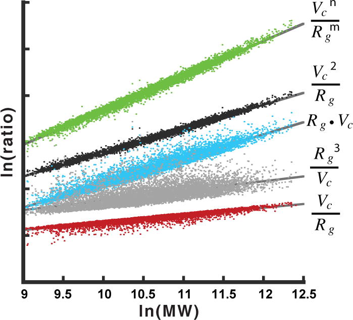
V_c and R_g were determined from theoretical atomic X-ray scattering profiles for 9,446 protein PDB²⁰ structures. For each profile, SAXS data were simulated to a maximum q = 0.5 Å⁻¹ (~13 Å). Various ratios of V_c and R_g against protein mass were examined in a log-log plot. The linear relationship observed for the ratio V_c² • R_g⁻¹ (black) suggests a power law relationship exists between the ratio and particle mass of the form ratio = c • (mass)^k. The ratio, V_c² • Rg⁻¹, is defined by units of ų with mass in Daltons. Additional ratios examined (green, cyan, gray and red) displayed asymmetric non-linear relationships. In green, the fit included m (0.9246 ± 0.0008) and n (1.892 ± 0.0005) in a non-linear surface optimization with an average mass error of 4.9 ± 4.3%. Fitting the linear power-law relationship (black) produces an average mass error of 4.0 ± 3.6%. Truncation of the data to q = 0.3 Å⁻¹ (~21 Å resolution) increases the mass error by 0.6% (Supplementary Fig. 2).

Figure 3. Power-law relationship betweenQrand particle mass (MW) allows direct mass determination.

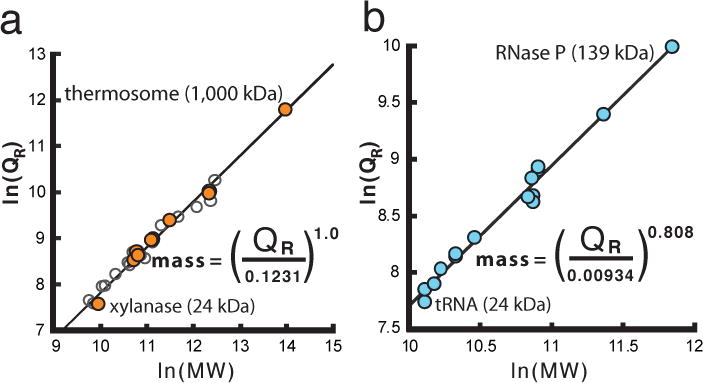
a, Qr calculated from previously reported experimental SAXS data for protein only samples (Supplementary Table 1). Gel-filtration purified samples (orange) were plotted with experimental data taken from BioIsis.net (open circles). c, Qr calculated from experimental SAXS data for RNA only samples (blue) (Supplementary Table 2). Final equations in a and b can be used for mass determination of protein or RNA only samples. Due to a lack of available SAXS data for protein-nucleic acid complexes, parameters for k and c remain undetermined.

V_c and R_g are both contrast and concentration independent, thus the determination of molecular mass using Qr can be made from SAXS data collected under diverse buffer conditions and concentrations, albeit free of interparticle interference. In fact, this linear relationship produced an average mass error < 4% for the 9,446 proteins in the in vacuo simulated dataset (Fig. 2).

Calculations of Qr from simulated and experimental (SI Tables 1 and 2) buffer-subtracted SAXS data of proteins, mixed protein-nucleic acid complexes or RNA alone (Fig. 3a, b) further verified the power-law relationship between Qr and mass. The mass errors for protein and RNA gel-filtration purified SAXS samples were 9.7 and 4.6%, respectively. Furthermore, for RNAs that were measured under folded and unfolded conditions, the average mass difference was 5.6%. The empirically determined mass power-law parameters (Fig. 3) are specific to macromolecular composition and analogous to empirical refractive index increments in light scattering studies²⁰. Moreover, Qr, as a mass estimator, assesses SAXS data quality for modeling. For heterogeneous samples, neither R_g nor V_c alone can reliably suggest a corrupted sample. Applying Qr to P4P6 and SAM-1 RNA samples with known contaminants¹⁰ (Table 1) shows that having 5 and 15% contaminants results in a 14 and 60% mass error, respectively, suggesting ab initio density models would not accurately represent the assumed homogenous solution state.

Cross-validating SAS model-data agreements

Atomistic modeling of SAS data relies on the reduced chi-square (chi²) error-weighted scoring function^{21, 22} that can be unreliable with moderately noisy datasets or over-estimated degrees-of-freedom (SI Fig. 4 and 5). This can lead to over-fitting and model misidentification. In crystallographic and NMR analyses, cross-validation statistical methods mitigate over-fitting and increase confidence in selected model(s)^{23, 24}. Here, we present an analogous robust statistical method based on the Nyquist-Shannon sampling and the noisy-channel coding theorems (SI Notes) for evaluating structural models against SAS data.

For a given maximum dimension (d_max), the sampling theorem⁹ determines that the number of unique, evenly distributed observations, n_s, required to represent a particle to a maximum scattering vector (q_max) is given by (d_max⋅q_max)⋅π ⁻¹. For example, SAS data to q_max of 0.3 Å⁻¹ determines for xylanase (d_max 44 Å) or 30S ribosomal particle (d_max 240 Å) the minimum number of observations are 4 and 23, respectively. This represents a ~20- to 125-fold over-sampling of a SAS curve composed of 500 observations. The Nyquist-Shannon limit (n_s) is the set of maximally independent observations from the band-limited SAS curve (SI Fig. 7). We reasoned that calculating chi² from a dataset reduced to n_s should more accurately assess the model-data agreement by restricting chi² evaluations to the set of independent random variables (SI Notes).

Due to over-sampling and the uncertainties in q, I(q) and d_max, determining the exact set of Nyquist-Shannon points will be difficult. Nevertheless, application of the noisy-channel coding theorem guarantees noise-free recovery of the SAS signal (SI Notes, Fig. 8 and 9); therefore, we propose the following sampling procedure for estimating chi² that partitions a SAS dataset into n_s equal bins for a given d_max. A randomly sampled data point is taken from each bin creating a n_s-length data vector that is used in chi². To minimize outlier influence, chi² is taken as the median over k sampling rounds (typically k = 1001) yielding a statistic we call X²_free. Analogous to R_free, X²_free uses a cross-validation scheme that excludes data from each bin during a round. This technique is akin to the robust least-trimmed squares method²⁵ and provides resistance to outliers, preventing over-fitting and the misidentification of models^{26, 27}.

Resisting over-fitting with X²_free

We tested X²_free on SAXS data for xylanase at pH 7.2 (Fig. 4a). Based on the fit to the crystallographic structure (PDB 1REF, chi² = 3.9), SAXS data implies an alternate conformation in solution. Using 1REF as a reference structure, 1,600 conformations were generated and used in a conventional all data chi² determination. ~7% of the models produced chi² < 1 suggesting data over-fitting with the best model (chi² = 1.0; Fig. 4a) showing a clear bias in the high q-region. Using X²_free, no model was identified with a X²_free < 1 and the best model (X²_free = 1.39) demonstrated improved fitting in the high q-region, showing X²_free distinguishes subtle conformational states. By minimizing on the median n-limited chi², X²_free more accurately determines the true model-data agreement and is not prone to over-fitting (SI Fig. 5).

Figure 4. Objective, quantitative evaluation of models using the least medianχ²(X²_free).

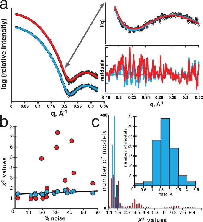
a, Selection of the best PDB model from a pool of 1,600 conformations generated using CONCOORD²⁹. The best selected model (model 44 of 1600) from CRYSOL (red) with a conventional χ² = 1 demonstrates a bias in the high q-region of the residuals whereas the best selected model (model 560 of 1600) using X²_free (cyan) displays an even distribution throughout the residuals with X²_free = 1.39. The bias within the high q region (0.18 Å⁻¹ < q < 0.24 Å⁻¹) implies a conformational difference between the data (red) and target model due to over-fitting. The resistance to over-fitting by X²_free enables the identification of different “best” models. b, Effects of noise on χ²-values from X²_free (cyan) and conventional χ² (red) calculations. Varying empirical noise levels were transposed onto a simulated SAXS profile of a randomly selected xylanase model generated by CONCOORD. A specified noise level represents the average noise in the last third of the q-range in a. Conventional χ² (red) is unstable and directly influenced by outliers producing erroneous χ²-values whereas X²_free is resistant and stable to noise (black line). Erroneous χ²-values will increase the false-negative rate for an experiment. c, Distribution of χ²-values determined from the set of models with an r.m.s.d < 1.5 at 19% noise. 30 randomly selected targets were fitted against 500 simulated SAXS curves at 19% noise from a pool of CONCOORD generated xylanase conformations. (Inset) Distribution of r.m.s.d for all models with a X²_free < 1.5. At higher noise, X²_free (cyan) produces narrower χ²-value distributions than conventional χ² (red) for near native conformations, thus reducing overall false negative rate.

To test how resistant X²_free is to noise, we simulated noisy xylanase SAXS datasets using empirical noise from reference datasets and evaluated how well conventional chi² and X²_free can identify the true model from a set of randomly perturbed structures. Under low noise (≤ 12%), both X²_free and conventional chi² behave similarly. At higher noise levels, conventional chi² becomes unstable, such that true models would be erroneously rejected. In contrast, X²_free values were stable over the tested noise levels and effective at identifying matches (Fig. 4b). More importantly, for near-native conformations of the target (root-mean-square difference, r.m.s.d < 1.5), conventional chi² values are widely distributed with nearly half greater than 2 (Fig. 4c). For X²_free, the distribution is narrower suggesting near native conformations are better identified with fewer false negatives.

Validating model-data resolution limits

Determining resolution limits of model-data agreements cannot be achieved by chi² alone and requires a metric we define as R_sas incorporating residuals between modeled and experimental values for both R_g and V_c given by:

$$R_{\text{SAS}}=\frac{{(R_g^{\text{exp}}-R_g^{\text{model}})}^2}{{\left(R_g^{\text{exp}}\right)}^2}+\frac{{(V_c^{\text{exp}}-V_c^{\text{model}})}^2}{{\left(V_c^{\text{exp}}\right)}^2}$$ (3)

R_sas is a difference distance metric determined from the set of Q-independent SAS invariants. Calculation of R_sas at varying resolutions provides an objective basis to determine appropriate resolution limits for data-model agreements. For dilute xylanase (SI Fig. 4a, 4b), data were collected to a maximum q = 0.5 Å⁻¹ (~13 Å resolution) and fit to PDB 1REF with a chi² of 1.3 suggesting an acceptable data-model agreement. However, inspection of R_sas and X²_free (20.3 and 1.8, respectively) reveal low agreement. Truncating the SAS data shows a significant decrease in R_sas with X²_free increasing initially then decreasing as the data-model agreement improves (SI Fig 4b). Convergence of R_sas towards zero with a X²_free ≤ 1.5 implies the limit of the data-model agreement to be q ≃ 0.2 Å⁻¹ or a resolution of 31 Å. The combination of R_sas and X²_free, for a given model, provides a quantitative and graphical approach for determining the acceptable resolution between the data and model (SI Fig. 4b and 5). As SAXS data is often used to filter a large set of conformationally distinct models, the models themselves may not be capable of describing the SAXS data to high resolution; therefore, application of R_sas and X²_free may provide the useful resolution of the data-model agreement. Nevertheless, as done recently for crystallography²⁷, a functional definition of resolution can come from the noisy-channel coding theorem. Here, the useful resolution of the data will be asserted by the highest Nyquist-Shannon point supported by the data.

Perspective

The SAS invariant V_c extends analysis to flexible biopolymers in solution. The volume-per-correlation length, like R_g, faithfully informs on the conformational state of the particle and can be calculated for models determined by other structural techniques including electron microscopy, X-ray crystallography, NMR and SANS. V_c provides a unique descriptor of the scattering experiment that is broadly applicable. We expect that V_c may further characterize voids in materials such as bone, polymeric beads or nano-materials. As the ratio of the square of V_c to R_g defines a mass parameter, Qr, SAS experiments can now inform on particle mass without requiring compactness and instrument calibration. Furthermore, X²_free is a robust statistical metric that we envision will enable cross-validated determination of flexible ensembles against observed SAXS data. We anticipate that V_c, Qr, X²_free, and R_sas will efficiently and objectively aid characterization of flexible macromolecules, check sample quality, determine mass and assembly states, detect concentration-dependent scattering, reduce model misidentification and over-fitting, and assess resolution for model to data agreement.

Methods

X²_free Calculation

For a given d_max, the SAXS/SANS data collected between q_min and q_max can be divided into n_s equal bins where n_s is determined by the Nyquist-Shannon sampling theorem⁹. Here, d_max is measured from the atomistic model; however, d_max can be directly inferred using an indirect Fourier transform method such as GNOM. In the case of 500 data points, and n_s = 10, each bin will contain 50 data points such that a single randomly selected datapoint will represent that Nyquist-Shannon point. Since a selected data point may be biased by interparticle interference or uncertainties in q or I(q), the selection of the representative datapoint from the Nyquist-Shannon bin must occur through several selection rounds (k). During each round, the set of randomly selected points comprises the test set for calculating chi² against the model. The accepted value is taken as the median over k rounds. The number of rounds, k, will vary with the average noise level of the SAXS/SANS dataset. The probability of selecting an erroneous datapoint from a bin scales directly with the noise. We have found for high quality data (< 10% noise), k can be as small as a few hundred whereas for high noise data, k should be 2000 to a maximum of 3000.

Sample preparation

Protein and RNA samples were derived from a variety of sources. For glucose isomerase and xylanase, protein samples were obtained as suspended crystals (Hampton Research). Each protein was further purified by gel-filtration chromatography immediately before SAXS data collection in buffer containing either (A) 20 mM HEPES pH 7.2, 5 mM MgCl₂, 100 mM KCl and 2 mM TCEP, (B) 40 mM MES pH 6.8, 8 mM MgCl₂, and 100 mM KCl, or (C) 40 mM NaCitrate pH 5.0, 75 mM KCl and 1% glycerol. Proteins were resuspended by a 50-fold dilution of the crystals in buffers A or B for glucose isomerase and buffers A, B or C for xylanase. Diluted crystals were incubated at 37 °C on a nutator for 1 hour, concentrated to 10 mg/ml and injected on a pre-equilibrated Superdex 200 PC 3.2 column (GE Healthcare) for glucose isomerase and Superdex 75 PC 3.2 column (GE Healthcare) for xylanase. Fractions corresponding to peak elution were taken for SAXS and quantitated by absorbance at 280 nm.

TAQ polymerase was recombinantly expressed and purified from Escherichia coli using cells transformed with pET vector conferring ampicillin resistance. Cells were grown at 37 °C, induced for 4 hours with IPTG at 0.8 OD₂₆₀ before harvesting. Cells were lysed as described³⁰. Lysate was clarified by low-speed spin in 50 mL falcon tubes and incubated at 65 °C for 20 minutes. Lysate was further clarified by high speed centrifugation at 20,000 × g for 40 minutes at 4 °C. Bound nucleic acids were removed by PEI treatment and ammonium sulfate precipitation. Protein was resuspended in buffer B and further purified to homogeneity using Superdex 200 HR 10/30 (GE Healthcare) for SAXS analysis.

Catalase (human erythrocyte) was purchased from a commercial source (EMD). 1 mg was resuspended in 100 uL of buffer A and further purified using a Superose 6 PC 3.2 column (GE Healthcare) equilibrated in buffer A. Fraction corresponding to peak elution was taken for SAXS analysis.

Thermosome from Sulfolobus solfataricus was purified from source and kindly provided by Steve Yannone (Lawrence Berkeley National lab). Thermosome samples were prepared by purification on a Superose 6 HR 10/30 column in buffer equilibrated with 40 mM pH 5.5, 75 mM KCl, 75 mM NaCl, 5 mM MgCl₂, and 2 mM TCEP. Fraction corresponding to peak elution was taken for SAXS analysis.

Data for Full-length and truncated TBL1 was kindly provided by Yoana Dimitrova and Walter Chazin (Vanderbilt University). Data for p65 was kindly provided by Andrea Berman and Tom Cech (University of Colorado at Boulder). Data for PYR1 samples were kindly provided by Kenichi Hitomi and Elizabeth Getzoff and purified as described¹¹. Samples were purified and analyzed onsite by gel-filration and MALS immediately before SAXS analysis.

Multi-angle light scattering (MALS)

Multi-angle light scattering (MALS) studies were performed inline with size-exclusion chromatography on protein and RNA samples to assess monodispersity and mass of the SAXS samples using an 18-angle DAWN HELEOS light scattering (LS) detector in which detector 12 was replaced with a DynaPro quasi-elastic light scattering detector (Wyatt Technology). Simultaneous concentration measurements were made with an Optilab rEX refractive index detector (Wyatt Technology) connected in tandem to the LS detector. For each buffer used, the MALS system was calibrated with BSA at 10 mg/mL to determine delay times and band broadening. For proteins, BSA, xylanase and glucose isomerase provided an additional calibration of the refractive index increment for protein samples. For RNA samples, the refractive index increment was determined from P4–P6 RNA samples^{10, 30}.

MALS analyses were performed on all the RNAs (except tRNA^phe) in this study and a set of proteins comprising glucose isomerase, xylanase, thermosome, catalase, TBL1, PYR1, and p65 (Table S1 and S2).

PDB query

The Protein Data bank (PDB) was used as a source for structural models for SAXS simulations. The comprehensive protein dataset was selected based on the following criteria: molecular mass range (10 to 1200 kDa), technique (X-ray crystallography), resolution limits (1.8 to 3.2 Å), exclude 90% similarity, protein only, and single models with 1 to 2 chains in the asymmetric unit. Further manual curation was performed for structures where the asymmetric unit produced two models physically separated in space without crystal contacts. For the RNA only datasets, the following criteria was used: RNA only, molecular mass range 10 to 250 kDa, exclude 95% similarity, technique (X-ray crystallography) and single model. Finally for mixed protein-nucleic acid complexes, the following criteria was used, molecular mass range 8 to 1000 kDa, technique (X-ray crystallography), protein and RNA, protein and DNA, 95% similarity and single model.

SAXS data collection

SAXS data were collected at beamline 12.3.1 of the Advanced Light Source at the Lawrence Berkeley National Laboratory². SAXS data were collected as a 2/3^rds dilution series using 20 uL samples and three different exposures. Exposures generally follow a short, medium and long time consisting of 0.1, 1 and 6 seconds or 0.5, 1 and 8 seconds and were merged as described¹⁰. Samples after gel-filtration purification eluted within the range of 1.5 and 3 mg/mL and for each sample, buffer was collected from the gel-filtration column after 1.2 column volumes for corresponding matching SAXS buffers.

For each sample, aggregation and interparticle interference was assessed using overlay plots of the concentration series in Gnuplot (http://www.gnuplot.org). Fits to the Guinier region (q⋅R_g < 1.3) were performed with software at beamline 12.3.1 (Robert Rambo, Lawrence Berkeley National Lab) and all data graphs were prepared with Kaleidagraph (http://www.synergy.com) and gnuplot. Figures with structural models were prepared with VMD and rendered with Povray (http://www.povray.org).

SAXS data analysis

For each SAXS dataset used in this study, linear fits to the Guinier region were performed with ruby scripts, rubyGSL (by Yoshiki Tsunesada) and the GNU Scientific Library (http://www.gnu.org/software/gsl/) for the determination of R_g and I(0). The Guinier parameters were subsequently used to calculate an extrapolated scattering dataset to zero angle at intervals determined from the average scattering vector increment, Δ_q.

Based on an extrapolated dataset, V_c was calculated by dividing the Guinier I(0) by the area of the transformed intensity taken as the product of q·I(q) and integrating using the trapezoid rule. For simulated atomic SAXS profiles, extrapolation was not necessary. Simulated atomic SAXS profiles were calculated with FOXS as it can calculate scattering profiles at specified scattering vector increments consistent with experimental measurements whereas CRYSOL (without an input SAXS dataset) can only calculate a maximum of 256 scattering intensities at a specified maximum scattering vector. Typical datasets collected at a maximum q of 0.32 Å⁻¹ at beamline 12.3.1 produce ~500 data points with the beamstop centered in the middle of the detector. Visual comparison of atomic SAXS profiles from FOXS with CRYSOL did not illustrate any systematic differences.

For experimental SAXS datasets that were fit to an input PDB model, CRYSOL was used with default input parameters. In these cases, CRYSOL reports chi and not chi-square for the model fits in the output log file.

Conformational Simulation

SAM-1 riboswitch molecular dynamics simulations were performed with CNS as described¹³. Briefly, the SAM crystal structure (PDB: 2GIS) was analyzed with FIRST and FRODA³¹ at several energy cut-offs to determine plausible rigid and flexible regions within the structure. These were used to ascribe constraints within the structure for molecular dynamic simulations with CNS using anneal.inp. The CNS input file was modified to remove the electrical potential from the energy function and calculations were performed as torsional angle dynamics only. For each simulation, 2000 steps were recorded in the trajectory file and each step was written to file as a PDB.

CONCOORD simulations with 1REF were performed with the following command line argument:

$$\text{disco -op disco -n 1}000\text{ -bump -damp 2 -viol 5 -t 1}00$$

to generate 1000 possible conformations close to the starting input structure. The resulting PDB files were fit to the experimental SAXS dataset with CRYSOL and the output intensity file for each PDB conformation was used to calculate V_c.

Simulating Noisy SAXS Datasets

SAS intensities over a single exposure will range over several decades and consequently, the noise levels will vary throughout the measured q-region. Therefore, we used intensity uncertainties from previously collected SAXS experiments as a source of realistic noise for the simulated SAXS datasets. The noise level of the empirical SAXS curve is reported as the average relative noise in the last third of the observed q-range (Fig. 4).

For a selected q, the simulated I(q) was randomly displaced based on a random draw using the Box-Muller transform of a standard Gaussian distribution parameterized by the empirical intensity, I(q)_obs, and uncertainty, error(q)_obs. The Box-Muller transform returns two possible values and a random binary selection was used to provide a final single value for the displacement of the simulated I(q), I(q)_displaced. The simulated error(q) was reported as I(q)_displaced * error(q)_obs/I(q)_obs.

References

- 1.Harrison SC. Comments on the NIGMS PSI. Structure. 2007;15:1344–1346. doi: 10.1016/j.str.2007.10.004. [DOI] [PubMed] [Google Scholar]
- 2.Hura GL, et al. Robust, high-throughput solution structural analyses by small angle X-ray scattering (SAXS) Nat Methods. 2009;6:606–612. doi: 10.1038/nmeth.1353. [DOI] [PMC free article] [PubMed] [Google Scholar]
- 3.Rambo RP, Tainer JA. Bridging the solution divide: comprehensive structural analyses of dynamic RNA, DNA, and protein assemblies by small-angle X-ray scattering. Curr Opin Struct Biol. 2010;20:128–137. doi: 10.1016/j.sbi.2009.12.015. [DOI] [PMC free article] [PubMed] [Google Scholar]
- 4.Sosnick TR, Woodson SA. New era of molecular structure and dynamics from solution scattering experiments. Biopolymers. 2011;95:503–504. doi: 10.1002/bip.21643. [DOI] [PubMed] [Google Scholar]
- 5.Glatter O, Kratky O. Small angle x-ray scattering. Academic Press; London ; New York: 1982. [Google Scholar]
- 6.Putnam CD, Hammel M, Hura GL, Tainer JA. X-ray solution scattering (SAXS) combined with crystallography and computation: defining accurate macromolecular structures, conformations and assemblies in solution. Q Rev Biophys. 2007;40:191–285. doi: 10.1017/S0033583507004635. [DOI] [PubMed] [Google Scholar]
- 7.Jacques DA, Trewhella J. Small-angle scattering for structural biology—expanding the frontier while avoiding the pitfalls. Protein Sci. 2010;19:642–657. doi: 10.1002/pro.351. [DOI] [PMC free article] [PubMed] [Google Scholar]
- 8.Bai Y, Das R, Millett IS, Herschlag D, Doniach S. Probing counterion modulated repulsion and attraction between nucleic acid duplexes in solution. Proc Natl Acad Sci U S A. 2005;102:1035–1040. doi: 10.1073/pnas.0404448102. [DOI] [PMC free article] [PubMed] [Google Scholar]
- 9.Moore P. Small-angle scattering. Information content and error analysis. Journal of Applied Crystallography. 1980;13:168–175. [Google Scholar]
- 10.Rambo RP, Tainer JA. Improving small-angle X-ray scattering data for structural analyses of the RNA world. RNA. 2010;16:638–646. doi: 10.1261/rna.1946310. [DOI] [PMC free article] [PubMed] [Google Scholar]
- 11.Nishimura N, et al. Structural mechanism of abscisic acid binding and signaling by dimeric PYR1. Science. 2009;326:1373–1379. doi: 10.1126/science.1181829. [DOI] [PMC free article] [PubMed] [Google Scholar]
- 12.Santiago J, et al. Modulation of drought resistance by the abscisic acid receptor PYL5 through inhibition of clade A PP2Cs. Plant J. 2009;60:575–588. doi: 10.1111/j.1365-313X.2009.03981.x. [DOI] [PubMed] [Google Scholar]
- 13.Stoddard CD, et al. Free State Conformational Sampling of the SAM-I Riboswitch Aptamer Domain. Structure. 2010;18:787–797. doi: 10.1016/j.str.2010.04.006. [DOI] [PMC free article] [PubMed] [Google Scholar]
- 14.Hammond JA, Rambo RP, Kieft JS. Multi-domain packing in the aminoacylatable 3′ end of a plant viral RNA. J Mol Biol. 2010;399:450–463. doi: 10.1016/j.jmb.2010.04.016. [DOI] [PMC free article] [PubMed] [Google Scholar]
- 15.Orthaber D, Bergmann A, Glatter O. SAXS experiments on absolute scale with Kratky systems using water as a secondary standard. Journal of Applied Crystallography. 2000;33:218–225. [Google Scholar]
- 16.Mylonas E, Svergun DI. Accuracy of molecular mass determination of proteins in solution by small-angle X-ray scattering. Journal of Applied Crystallography. 2007;40:s245–s249. [Google Scholar]
- 17.Fischer H, de Oliveira Neto M, Napolitano HB, Polikarpov I, Craievich AF. Determination of the molecular weight of proteins in solution from a single small-angle X-ray scattering measurement on a relative scale. Journal of Applied Crystallography. 2009;43:101–109. [Google Scholar]
- 18.Rambo RP, Tainer JA. Characterizing flexible and intrinsically unstructured biological macromolecules by SAS using the Porod-Debye law. Biopolymers. 2011;95:559–571. doi: 10.1002/bip.21638. [DOI] [PMC free article] [PubMed] [Google Scholar]
- 19.Berman HM, et al. The Protein Data Bank. Nucleic Acids Res. 2000;28:235–242. doi: 10.1093/nar/28.1.235. [DOI] [PMC free article] [PubMed] [Google Scholar]
- 20.Wyatt PJ. Light scattering and the absolute characterization of macromolecules. Anal Chim Acta. 1993;272:1–40. [Google Scholar]
- 21.Svergun D, Barberato C, Koch MHJ. CRYSOL – a Program to Evaluate X-ray Solution Scattering of Biological Macromolecules from Atomic Coordinates. Journal of Applied Crystallography. 1995;28:768–773. [Google Scholar]
- 22.Schneidman-Duhovny D, Hammel M, Sali A. FoXS: a web server for rapid computation and fitting of SAXS profiles. Nucleic Acids Res. 2010;38:W540–544. doi: 10.1093/nar/gkq461. [DOI] [PMC free article] [PubMed] [Google Scholar]
- 23.Brunger AT. Free R value: a novel statistical quantity for assessing the accuracy of crystal structures. Nature. 1992;355:472–475. doi: 10.1038/355472a0. [DOI] [PubMed] [Google Scholar]
- 24.Brunger AT, Clore GM, Gronenborn AM, Saffrich R, Nilges M. Assessing the quality of solution nuclear magnetic resonance structures by complete cross-validation. Science. 1993;261:328–331. doi: 10.1126/science.8332897. [DOI] [PubMed] [Google Scholar]
- 25.Rousseeuw PJ, Leroy AM. Robust regression and outlier detection. Wiley; New York: 1987. [Google Scholar]
- 26.Jie Y, Qi T, Amores J, Sebe N. Toward Robust Distance Metric Analysis for Similarity Estimation. Computer Vision and Pattern Recognition, 2006 IEEE Computer Society Conference on. 2006;1:316–322. [Google Scholar]
- 27.Karplus PA, Diederichs K. Linking crystallographic model and data quality. Science. 2012;336:1030–1033. doi: 10.1126/science.1218231. [DOI] [PMC free article] [PubMed] [Google Scholar]
- 28.Brunger AT, et al. Crystallography & NMR system: A new software suite for macromolecular structure determination. Acta Crystallogr D Biol Crystallogr. 1998;54:905–921. doi: 10.1107/s0907444998003254. [DOI] [PubMed] [Google Scholar]
- 29.de Groot BL, et al. Prediction of protein conformational freedom from distance constraints. Proteins. 1997;29:240–251. doi: 10.1002/(sici)1097-0134(199710)29:2<240::aid-prot11>3.0.co;2-o. [DOI] [PubMed] [Google Scholar]
- 30.Rambo RP, Doudna JA. Assembly of an active group II intron-maturase complex by protein dimerization. Biochemistry. 2004;43:6486–6497. doi: 10.1021/bi049912u. [DOI] [PubMed] [Google Scholar]
- 31.Fulle S, Gohlke H. Analyzing the flexibility of RNA structures by constraint counting. Biophys J. 2008;94:4202–4219. doi: 10.1529/biophysj.107.113415. [DOI] [PMC free article] [PubMed] [Google Scholar]
Associated Data
This section collects any data citations, data availability statements, or supplementary materials included in this article.