Neopolyploidy and diversification in Heuchera grossulariifolia

Abstract

Newly formed polyploid lineages must contend with several obstacles to avoid extinction, including minority cytotype exclusion, competition, and inbreeding depression. If polyploidization results in immediate divergence of phenotypic characters these hurdles may be reduced and establishment made more likely. In addition, if polyploidization alters the phenotypic and genotypic associations between traits, i.e. the P and G matrices, polyploids may be able to explore novel evolutionary paths, facilitating their divergence and successful establishment. Here we report results from a study of the perennial plant Heuchera grossulariifolia in which the phenotypic divergence and changes in phenotypic and genotypic covariance matrices caused by neopolyploidization have been estimated. Our results reveal that polyploidization causes immediate divergence for traits relevant to establishment and results in significant changes in the structure of the phenotypic covariance matrix. In contrast, our results do not provide evidence that polyploidization results in immediate and substantial shifts in the genetic covariance matrix.

Introduction

Polyploidy, having more than two sets of chromosomes, is widespread among a diverse array of taxa, especially in plants, but also occurring infrequently among animals (Otto and Whitton 2000; Soltis 2005). In order for a newly formed polyploid lineage (hereafter neopolyploid) to avoid extinction it must overcome several formidable hurdles. Arguably, the largest of these is minority cytotype exclusion (Levin 1975). Since a neopolyploid invariably arises within a larger diploid population, the majority of its reproduction will be with diploid individuals. Because these intercytotype matings typically produce inviable offspring, the result is frequency dependent selection against the minority cytotype and its inevitable extinction (Felber 1991). In addition, competition with the diploid progenitor, reduced fecundity, and inbreeding depression due to small population sizes are all arrayed against neopolyploid establishment (Otto and Whitton 2000; Ramsey and Schemske 2002; Otto 2007).

Phenotypic divergence in the neopolyploid lineage may reduce these hurdles and facilitate establishment. For instance, divergence in flowering phenology may provide some reduction in minority cytotype disadvantage by facilitating assortative mating (Husband and Sabara 2004). In addition, phenotypic divergence in other traits relevant to ecological niche use may yield reduced competition with diploid progenitors (Otto and Whitton 2000; Buggs and Pannell 2007; Parisod et al. 2010). Several studies have compared the phenotypes of diploids and polyploids. However, these studies often include species that have undergone a polyploidization event at an unknown time in the past, and therefore compare the diploid ancestor with an evolved polyploid lineage (Burton and Husband 2000; Nuismer and Thompson 2001; Buggs and Pannell 2007; Halverson et al. 2008). The difficulty here is that changes in phenotype may be due to polyploidy or to changes in gene frequency caused by selection or drift after the polyploidization event (Levin 1983). Though a significant proportion of the research on polyploidy is of this type, a possibly more fruitful line of research is to create autopolyploids synthetically and study the resulting phenotypic changes (Husband et al. 2008). Although studies using synthetic autopolyploids appear in the crop science literature, few studies employ genetically variable non-domesticated species and track family structure (Husband et al. 2008).

Establishment and persistence of polyploid lineages may also be facilitated by changes in phenotypic covariance structure. Specifically, changes in the phenotypic covariance matrix (P matrix) may allow selection to push polyploids in novel directions within phenotypic space not accessible to ancestral diploids and thus allow their rapid diversification (Schluter 1996; Steppan 1997). Though clearly relevant, P is rarely estimated in polyploid studies (but see Nuismer and Cunningham 2005).

Polyploid establishment may also be aided by changes in the genetic covariance matrix. Specifically, if polyploidization opens up new lines of genetic variation (Osborn et al. 2003) which are inaccessible to diploids, evolution may result in the rapid divergence of polyploid lineages (Soltis and Soltis 2000). Importantly, because the evolutionary response to natural selection is constrained by the genetic covariance matrix (Lande 1979), changes in G associated with polyploidy may allow polyploids to diversify rapidly even if diploid and polyploids experience identical patterns of phenotypic selection. Although empirical evidence suggests that G changes relatively slowly within species (Steppan 1997; Begin and Roff 2003) we know nothing about the impact of polyploidization per se on G, though recent studies in allopolyploids have documented rapid changes in epigenetic effects, gene regulation and expression (Liu and Wendel 2003; Comai 2005; Chen and Ni 2006; Gaeta et al. 2007; Buggs et al. 2009; Flagel and Wendel 2009).

Theoretical predictions regarding the affect of polyploidy on G are limited. Gallias (2003) predicts that if the phenotypic range for the trait being examined is the same for diploids and autotetraploids, the additive variance will be less in autotetraploids than diploids. If however, the phenotypic range is different between the ploidies, then autotetraploids may exhibit either more or less additive variance. Gallias does not make any predictions regarding the covariance entries of G. We therefore developed a n-loci diallelic model to examine whether a change in ploidy level affects G (Appendix 1). From this model we predict that polyploidy will alter the G matrix only in as much as it alters patterns of gene regulation and pleiotropy. Thus, empirical studies in autopolyploids are necessary before general conclusions can be formed.

Here we use synthetic autotetraploid Heuchera grossulariifolia to elucidate the phenotypic and genetic changes that accompany autopolyploidization. We examine two distinct populations and study several phenotypic traits which previous work has shown to be under selection and important in intraspecific and interspecific interactions (Nuismer and Cunningham 2005; Nuismer and Ridenhour 2008; Thompson and Merg 2008). Our goal is to address the following questions: 1) Are neopolyploids phenotypically differentiated from diploids, and are these effects consistent across polyploidy origins? 2) Does the P matrix of neopolyploids differ, and if so, are differences consistent across polyploidy origins? 3) Does the G matrix of neopolyploids differ, and if so, are differences consistent across polyploidy origins?

Methods

Heuchera grossulariifolia is a perennial Saxifrage commonly found in Washington, Idaho, and Montana where it grows in greatest abundance along the major river drainages of the region. Within this region, both diploid and autotetraploid H. grossulariifolia exist and populations of pure diploids, pure autotetraploids, and mixed ploidy have been identified and studied extensively (Wolf et al. 1990; Thompson et al. 1997; Segraves et al. 1999; Nuismer and Cunningham 2005; Nuismer and Ridenhour 2008; Thompson and Merg 2008). This study focused on two exclusively diploid Idaho populations: one located along the South Fork Salmon River (SFS), and the other along the North Fork Clearwater River (NFC) (Figure 1).

Figure 1. Map of Northern Idaho highlighting study populations.

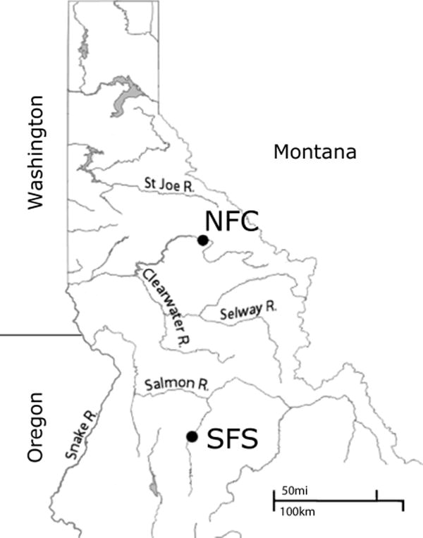
The two study populations, North Fork Clearwater (NFC) and South Fork Salmon (SFS) shown as large filled circles.

Seeds from multiple plants from each population were collected during the summer of 2005. Seeds from each plant were stored in separate glassine bags until germination during the winter of 2005–2006. In December of 2005, approximately 150 seeds from each of ten plants from the NFC and SFS populations were planted in 7.6 cm square pots (30 seeds per pot). Due to an equipment failure, SFS seedlings suffered high levels of mortality, necessitating the replanting of a new set of the SFS population seeds in March 2006. Five weeks after planting, approximately 100 haphazardly selected seedlings per maternal plant were treated with colchicine solution (980ml DH₂0, 10.53g colchicine, 20ml DMSO, 2ml Tween80) to induce polyploidy. Specifically, ten seedlings at a time were placed in a folded paper towel and placed into a 250 ml bottle with 10 ml colchicine solution for 48 hours in a rotating device to repeatedly bathe the seedlings. In order to create an equivalent diploid population against which to compare our neopolyploids, seedlings also went into bottles with 10ml H₂0 in the rotating device for 48 hours at the same time as the colchicine-treated seedlings. After removal from the rotating device, seedlings were planted individually in 72 place trays, with the water-treated seedlings planted among the colchicine treated seedlings in randomly selected spots. In total, we planted 983 seedlings treated with colchicine (NFC: 433, SFS: 450), and 172 seedlings treated only with water (NFC: 82, SFS: 90). Plants were then grown in a growth chamber with 16 hours of artificial light per day and watered as needed.

Approximately 16 weeks after planting, two leaves per plant were sampled to determine ploidy by flow cytometry following protocols in Arumuganathan and Earle (1991) with the addition of PVP-40 in the chopping buffer to reduce phenolic impurities. A total of 96 plants, including 21 from the NFC population and 75 plants from the SFS population were putatively converted to tetraploids. All plants were transplanted to 10.2 cm square pots and moved into a greenhouse at 20 weeks after planting. Inducing polyploidy through colchicine can create chimeric plants that are part diploid and part tetraploid and so we verified the ploidy of putative tetraploid plants again at approximately 40 weeks after planting. The final number of tetraploids remaining after this second round of flow cytometry was 56; 19 were from the NFC population and 37 plants from the SFS population.

Because the colchicine treatment caused higher mortality (63.1% mortality for colchicine treated plants versus 14.9% for H₂O treated) and appeared to reduce growth rates, the neopolyploid and diploid comparison plants were overwintered in the greenhouse and crossed in the spring of 2007 to create an F1 generation for each ploidy and population. Specifically, for the NFC population, five tetraploid plants and five diploid plants were crossed within ploidy in a full diallel design (Lynch and Walsh 1998), producing 20 tetraploid and 20 diploid families. We were able to use only five plants for this population because only five of the neopolyploids flowered. For the SFS population, 18 tetraploids flowered and so 18 tetraploid plants and 18 diploid plants were crossed within ploidy using a partial diallel design (Lynch and Walsh 1998) with each plant being crossed four times for a total of 72 tetraploid and 72 diploid families. Crosses were performed by manually moving pollen using a pin under a dissecting microscope. The pin was sterilized by alcohol and flame between crosses. Since H. grossulariifolia is self-incompatible (Wolf et al. 1990; Thompson and Merg 2008), flowers were not emasculated. We verified that unintentional pollination did not occur by monitoring flowers that were not manually pollinated. Only manually pollinated flowers produced seeds. From each successful cross (all NFC crosses, 65 SFS diploid, 69 SFS tetraploid) seeds were collected from pollinated flowers in the summer of 2007 and 30 seeds were planted in the fall of 2007 in 7.6 cm square pots. After germination, 10 seedlings from each pot were haphazardly selected and transplanted into individual three-inch square pots and raised in a greenhouse at 24° C and a 16-hour day provided by a combination of natural and artificial light. Plants were spatially arranged in the greenhouse randomly, and were shuffled haphazardly approximately every 10 days to reduce environmental effects. When the F1 tetraploid plants were large enough, ploidy was verified through flow cytometry.

Trait measurement

Approximately every 4–5 weeks the number of leaves on each plant was counted to serve as a measure of growth rate. These leaf counts were completed a total of five times. During flowering, the number of open flowers per plant was recorded each day for all plants that flowered (SFS – 167 2x, 97 4x; NFC – 104 2x, 23 4x). Also during flowering, four open flowers per plant were photographed on a ruler, and the width of each flower measured using the imaging software ImageJ (Rasband 1997–2009). Since previous studies using H. grossulariifolia found that floral traits were highly correlated (Segraves and Thompson 1999), we chose to only measure flower corolla width (hereafter flower width), excluding other measurements such as flower length, pedicel length, etc. After all flowers on a scape had opened, the scape height was measured from the base of the plant. From this data, the following traits were analyzed: growth rate (leaves/day), average flower width, average scape height, number of scapes, average flowering day, maximum floral display (greatest number of flowers open at a time), and flowering days (number of days with flowers open). Average flowering day was calculated as in Nuismer and Cunningham (2005). Sample sizes for each trait, ploidy, and population are shown in Table 1.

Table 1.

Sample sizes for each population and generation

				Number of plants for which the trait was measured
population	generation	ploidy	total number of plants	growth rate	average flower date	flower width	maximum floral display	flowering days	scape height	number of scapes
NFC	F1	2	200	200	104	102	104	104	103	104
		4	198	198	23	23	23	23	22	23
	P	2	5	0	0	5	5	5	5	5
		4	5	0	0	5	5	5	5	5
	Natural	2	5	0	0	4	0	0	2	0
SFS	F1	2	548	548	166	159	166	166	130	170
		4	494	494	97	95	97	97	80	98
	P	2	18	0	0	13	0	0	18	0
		4	18	0	0	15	0	0	16	0
	Natural	2	9	0	0	4	0	0	5	0

Analyses of mean phenotypes

Statistical tests were conducted using the R statistical package (R Development Core Team 2009). Each trait was tested within population and ploidy for normality using the Shapiro-Wilk test. The null hypothesis of normality was rejected for all traits except average flower width (average p-value = 0.472), and average scape height (average p-value = 0.505). We first used a MANOVA to test for significant effects of population and ploidy. Traits that were not normally distributed were first transformed using a Box-Cox transform (Sokal and Rohlf 1995). Next, we tested for differences in means of individual traits across ploidies and populations using Wilcoxon Rank-Sum non-parametric tests if the untransformed data was non-normal, and Welch two sample t-tests if the untransformed data was normal.

Analyses of phenotypic covariance matrices

Phenotypic covariance matrices (P matrices) were calculated in R using Pearson’s method. Only plants that flowered were included in the P matrix calculations (NFC 2x: 104, NFC 4x: 23, SFS 2x: 167, SFS 4x: 97). We used a bootstrap test to determine: 1) if the variances and covariances were significantly different than zero within each ploidy and population, and; 2) to test whether the variances and covariances differed significantly across ploidies. Specifically, we first partitioned the data by population and ploidy creating four subsets (NFC 2x, NFC 4x, SFS 2x, SFS 4x), then for each of these subsets we assembled 10,000 bootstrap replicates of the appropriate size (above) by randomly sampling individuals from the partitioned data with replacement. Next, we calculated and stored the P matrix for each of these 10,000 bootstrap replicates. These 10,000 P matrices were used as the null distributions for the entries in the P matrices. In each case we compared the null distributions against zero, for variance components this was a one-tailed test, and for covariance components a two-tailed test. To generate distributions of the differences in the entries in P across ploidies, we simply subtracted the null distribution for diploids from that of tetraploids to yield two distributions of differences in P matrices, one for each population. As before, we compared the distributions of differences to zero, but in this case all tests were two-tailed. We also examined the effects of population and ploidy on the P matrices using the MANOVA jacknife approach outlined by Roff (Roff 2002; Roff and Mousseau 2005). In addition, we compared the structure of the P matrices using the Flury hierarchy outlined by Phillips and Arnold (1999) using the CPC software.

Analyses of genetic covariance matrices

We used the MCMCglmm method in the R package MCMCglmm (Hadfield 2010) to fit generalized linear mixed models to the phenotypic data and estimate the G matrices. The MCMCglmm package utilizes the known pedigree for all the plants to estimate the variance structures using Markov Chain Monte Carlo (MCMC) methods. Gallias (2003) shows that with half-sibs, the autotetraploid covariance is V_a/4 + V_d/36, where V_a is the additive variance and V_d is the dominance variance. We assume that the dominance variance is small relative to the additive variance and thus its contribution to the covariance is negligible. Each MCMC chain was run for 550,000 iterations, with a 50,000 iteration burn-in. Due to the limited number of flowering plants, we restricted our G matrix to the four traits of primary interest: flower width, scape height, average flowering date, and growth rate. Since the MCMCglmm package uses pedigree information to estimate G, we included all the F1 generation plants and the relevant P generation and natural plants for a total of 786 diploid (210 NFC, 576 SFS), and 715 tetraploid (203 NFC, 512 SFS) individuals in the analysis (See Table 1 for trait sample sizes). We initially attempted to use uniform (improper) priors, however the MCMC chain did not converge. Therefore, we used a proper prior, i.e. a prior whose probability density function integrates to one. We chose to base the prior on the P matrix, as it is generally a good estimate of G (Steppan et al. 2002). More specifically, we used an inverse Wishart distribution centered on P as the prior (Hadfield 2010). We found that the prior was generally informative, that is using different priors affected the estimated G, and therefore we used two different methods to generate priors. First, we calculated P for data pooled over population and ploidy. This method is biased towards finding no difference in G matrices, and thus provides a conservative test for differences in G. In the second method, we calculated the P matrix for each combination of population and ploidy separately, resulting in four P matrices. We then used these four P matrices as the prior for their respective population and ploidy and estimated the G matrix for each again. This method is biased towards finding differences in G, due to the different priors, and thus provides a conservative test of equality of G matrices.

An advantage of the MCMC method is that it can provide credible intervals for the elements, eigenvalues, and eigenvectors of G. In order to test for differences in the G matrices, we calculated the likelihood that a given parameter value could have occurred in both ploidy’s posterior distribution. Specifically, we determined the portions of the distributions that overlapped at the 95% level, and multiplied these probabilities. This test assumes that the two posterior distributions are independent. In the case of the combined priors method, this is obviously not the case, and the posterior distributions may be non-independent in the separate priors method due to relatedness of individuals. However, since both methods are like to produce positive correlation between distributions, this test is actually conservative.

We calculated the posterior distribution of eigenvalues for all G matrices in order to test the dimensionality of G, which is a measure of the number of genetically independent traits represented by a set of related phenotypic traits (Hine and Blows 2006). In addition, we calculated the posterior distribution of eigenvectors to aid in comparison of the G matrices. When estimating the G matrix of polyploids, the genetic variance attributed to additive affects may be inflated due to an extra dominance variance component not present in diploids (Gallais 2003) which we are unable to estimate. However, the contribution of this dominance variance component is likely to be small (Gallais 2003). Due to the relatively sparse NFC tetraploid data, the estimation of G in this case may be largely driven by the prior, but we have decided to include the NFC tetraploid data in the analysis for the sake of completeness.

Results

Mean phenotypes

The MANOVA revealed a significant effect of ploidy and population for multiple traits (Table 2). Wilcoxon Rank-Sum tests and t-tests for differences in means conducted within population and ploidy showed that in both populations tetraploid plants grew slower, had fewer scapes, flowered fewer days, and had larger flowers (Table 3). In the SFS population, tetraploids flowered later than diploids, and had a smaller maximum floral display. Scape height was not significantly different when comparing ploidies within populations.

Table 2.

MANOVA of trait by trait comparisons

		Df	Sum Sq	Mean Sq	F value	Pr(> F)
Growth rate	ploidy	1	0.028941	0.028941	52.23	< 0.0001	***
	pop	1	0.239399	0.239399	432.044	< 0.0001	***
(Box-Cox transformed, λ = 1.15)	ploidy:pop	1	0.016339	0.016339	29.487	< 0.0001	***
	Residuals	326	0.180639	0.000554
Average flower date	ploidy	1	1.02 × 10−11	1.02 × 10−11	0.1399	0.7086
	pop	1	1.42 × 10−8	1.42 × 10−8	195.2406	< 0.0001	***
(Box-Cox transformed, λ = − 1.74)	ploidy:pop	1	4.84 × 10−11	4.84 × 10−11	0.6635	0.4159
	Residuals	326	2.38 × 10−8	7.29 × 10−11
Flower width	ploidy	1	36.43	36.43	176.3564	< 0.0001	***
	pop	1	53.472	53.472	258.8548	< 0.0001	***
	ploidy:pop	1	0.609	0.609	2.9503	0.08681	.
	Residuals	326	67.342	0.207
Scape height	ploidy	1	82.7	82.7	1.3696	0.242733
	pop	1	458.9	458.9	7.5974	0.006174	**
	ploidy:pop	1	76.5	76.5	1.2673	0.261105
	Residuals	326	19689.4	60.4
Flowering	ploidy	1	22.793	22.793	75.7528	< 0.0001	***
	pop	1	23.184	23.184	77.0516	< 0.0001	***
(Cube root transformed)	ploidy:pop	1	1.595	1.595	5.3019	0.02193	*
	Residuals	326	98.088	0.301
Maximum floral display	ploidy	1	369.1	369.1	13.3813	0.000296	***
	population	1	69.9	69.9	2.5348	0.112328
(Box-Cox transformed, λ = 0.89)	ploidy:pop	1	4.1	4.1	0.1484	0.700281
	Residuals	326	8992.9	27.6
Number of Scapes	ploidy	1	21.084	21.0841	50.9473	< 0.0001	***
	pop	1	6.605	6.6046	15.9594	< 0.0001	***
	ploidy:pop	1	2.498	2.4984	6.0372	0.01453	*
	Residuals	326	134.912	0.4138
		DF	Pillai	approx F	num DF	den DF	Pr(> F)
Combined Effects	ploidy	1	0.59574	67.368	7	320	< 0.0001	***
	pop	1	0.75841	143.508	7	320	< 0.0001	***
	ploidy:pop	1	0.12208	6.357	7	320	< 0.0001	***
	Residuals	326

Table 3.

Tests for differences in trait means

				W = Wilcoxon Rank-Sum Tests, t = Welch Two Sample t-test
Trait	Pop	Ploidy	Mean	NFC 4x	SFS 2x	SFS 4x
growth rate	NFC	2	1.157E − 01	W = 31870 p < 0.0001	W = 7994 p < 0.0001	W = 37213 p < 0.0001
	NFC	4	8.753E − 02		W = 3451 p < 0.0001	W = 15041 p < 0.0001
	SFS	2	1.939E − 01			W = 250243 p < 0.0001
	SFS	4	1.255E − 01
average flower date	NFC	2	2.286E + 02	W = 1061 p = 0.400	W = 15676 p < 0.0001	W = 8757 p < 0.0001
	NFC	4	2.297E + 02		W = 3624 p < 0.0001	W = 2081 p < 0.0001
	SFS	2	1.887E + 02			W = 5838 p < 0.001
	SFS	4	1.971E + 02
flower width	NFC	2	4.337E + 00	t = −5.61 p < 0.0001	t = 15.1 p < 0.0001	t = −1.26 p = 0.211
	NFC	4	5.089E + 00		t = 13.0 p < 0.0001	t = 5.070 p < 0.0001
	SFS	2	3.436E + 00			t = −18.3 p < 0.0001
	SFS	4	4.422E + 00
maximum floral display	NFC	2	1.738E + 01	W = 1492 p = 0.00639	W = 10198 p = 0.0157	W = 6917.5 p < 0.0001
	NFC	4	1.443E + 01		W = 1901.5 p = 0.94	W = 1310.5 p = 0.194
	SFS	2	1.592E + 01			W = 9361 p = 0.0348
	SFS	4	1.287E + 01
flowering days	NFC	2	4.413E + 01	W = 1879 p < 0.0001	W = 13458 p = p < 0.0001	W = 8905 p < 0.0001
	NFC	4	2.304E + 01		W = 1779.5 p = 0.57	W = 1399.5 p = 0.0585
	SFS	2	2.401E + 01			W = 10977 p < 0.0001
	SFS	4	1.616E + 01
scape height	NFC	2	1.917E + 01	t = 0.844 p = 0.405	t = −2.07 p = 0.0393	t = −2.69 p = 0.00803
	NFC	4	1.797E + 01		t = −2.19 p = 0.0351	t = −2.71 p = 0.00939
	SFS	2	2.118E + 01			t = −0.934 p = 0.351
	SFS	4	2.231E + 01
number of scapes	NFC	2	3.231E + 00	W = 1921.5 p < 0.0001	W = 12251.5 p < 0.0001	W = 8077.5 p < 0.0001
	NFC	4	1.565E + 00		W = 1434.5 p = 0.0266	W = 1074.5 p = 0.696
	SFS	2	2.187E + 00			W = 10341 p = 0.000648
	SFS	4	1.633E + 00

Phenotypic covariance matrices

Several covariances were found to be significantly different than zero (Table 4). The bootstrap test also unsurprisingly revealed that the variance components (the diagonal entries in P) were all significantly different than zero. In addition, for all population and ploidy combinations we found a significant positive covariance between number of scapes and maximum floral display and between number of scapes and length of flowering period. Scape height positively covaried with maximum floral display for all groups except the NFC tetraploids. Flower width positively covaried with number of scapes for all but the SFS tetraploids. For the NFC groups, flower width also positively covaried with both maximum floral display and number of scapes. Flower width negatively covaried with average flowering day in the diploid groups, but not the tetraploid groups. Growth rate only significantly covaried with average flowering date in one group, SFS tetraploids, and it was a negative covariance. In summary, all variance entries in all P matrices were significantly different than zero, and on average half of the 21 covariances were also significantly different than zero.

Table 4.

P matrices

NFC 2X	growth rate	avg flower date	flower width	max floral display	flowering days	scape height	number of scapes
growth rate	.000664***	0.0355	−0.00147	−0.0120	−0.115*	0.00839	−0.00803*
avg flower date		970.7***	−6.28***	−51.4*	−31.2	−3.30	−11.5*
flower width			0.269***	0.806*	4.96***	0.234	0.328***
max floral display				48.1***	63.6***	14.9**	6.50***
flowering days					537.6***	23.9	28.6***
scape height						43.5***	−0.438
number of scapes							3.03***

NFC 4X	growth rate	avg flower date	flower width	max floral display	flowering days	scape height	number of scapes
growth rate	0.000196***	−0.0197	−0.00329**	−0.0122	0.0314	0.0115	0.00171
avg flower date		482.9***	−3.46	−39.2	−69.3	−67.8*	−4.71
flower width			0.352***	0.985*	3.29*	0.772	0.288*
max floral display				17.9***	26.6*	6.56	1.97**
flowering days					199.E***	32.7	8.84***
scape height						35.8***	1.58
number of scapes							0.712***

SFS 2X	growth rate	avg flower date	flower width	max floral display	flowering days	scape height	number of scapes
growth rate	0.00145***	−0.0348	0.000243	−0.00762	0.0000191	−0.0320	0.00225
avg flower date		329.7***	−1.58***	1.11	−19.3	−37.6***	2.44
flower width			0.148***	0.256	1.78***	0.287	0.0839*
max floral display				74.8***	65.7***	35.6***	7.84***
flowering days					205.2***	36.5***	14.7***
scape height						67.6***	1.80*
number of scapes							1.91***

SFS 4X	growth rate	avg flower date	flower width	max floral display	flowering days	scape height	number of scapes
growth rate	0.000653***	−0.156**	0.00114	0.0280*	0.0360	0.0541*	0.00241
avg flower date		350.4***	−1.60**	−10.0	−23.2	−45.6**	−2.40*
flower width			0.187***	0.173	0.531	0.941**	−0.0691
max floral display				31.9***	23.3***	24.8***	2.00***
flowering days					73.8***	12.1	4.71***
scape height						75.6***	−1.36*
number of scapes							0.775***

NFC 4X–2X	growth rate	avg flower date	flower width	max floral display	flowering days	scape height	number of scapes
growth rate	−0.000467***	−0.0553	−0.00182	−0.000256	0.0147	0.00307	0.00974
avg flower date		−487.8	2.82	12.2	−38.2	−64.5	6.77
flower width			0.0839	0.179	−1.66	0.538	−0.0390
max floral display				−30.2***	−37.0	−8.32	−4.53***
flowering days					−338.3***	8.79	−19.8***
scape height						−7.67	2.02
number of scapes							−2.32***

SFS 4X–2X	growth rate	avg flower date	flower width	max floral display	flowering days	scape height	number of scapes
growth rate	−0.000800***	−0.121	0.000901	0.0356	0.0360	0.0861*	0.000154
avg flower date		20.7	−0.0208	−0.111	−3.87	−8.00	−4.84*
flower width			0.0389	−0.0830	−1.24*	0.655	−0.153**
max floral display				−42.8***	−42.4**	−10.8	−5.83***
flowering days					−131.5***	−24.4*	−10.0***
scape height						7.98	−3.15**
number of scapes							−1.14***

The bootstrap test also revealed that some of the differences between the covariances in the tetraploid and diploid P matrices were of greater magnitude than expected by chance. In both populations, diploids had larger positive number of scapes by maximum floral display covariances, and larger positive number of scapes by flowering days covariances. For the SFS population, tetraploids had a larger growth rate by scape height covariance, and number of scapes negatively covaried with all traits except growth rate. In addition, the bootstrap test showed that tetraploids in both populations had significantly smaller variances for growth rate, maximum floral display, flowering days, and number of scapes for both the NFC and SFS populations. The MANOVA jacknife analysis of the P matrices showed a significant effect of ploidy, population, and the interaction between ploidy and population (Table 5). The Flury Hierarchy analysis revealed that for both NFC and SFS populations, using the “jump-up” approach, the diploid and tetraploid matrices shared some but not all principal components (Table 6). Specifically, the SFS population diploids had three of seven principal components in common with the SFS tetraploids, and the NFC population diploids shared four of seven principal components with tetraploids.

Table 5.

MANOVA Jacknife analysis of P matrices

	DF	Pillai	approx F	num DF	den DF	Pr(> F)
ploidy	1	0.99988	184554	28	644	< 0.00001 ***
population	1	0.99912	26040	28	644	< 0.00001 ***
ploidy:population	1	0.99902	23393	28	644	< 0.00001 ***
Residuals	671

Table 6.

Flury Hierarchy for P matrices

	NFC			SFS
Model	Chi Squared	DF	p-value	Chi Squared	DF	p-value
Equality	75.886	28	0	114.86	28	0
Proportional	56.797	27	0.0007	89.183	27	0
CPC	36.392	21	0.0198	46.122	21	0.0012
CPC(5)	34.325	20	0.024	46.122	20	0.0008
CPC(4)	30.123	18	0.0363	39.273	18	0.0026
CPC(3)	24.161	15	0.0624	37.792	15	0.001
CPC(2)	18.078	11	0.0798	18.938	11	0.0622
CPC(1)	8.086	6	0.2319	10.325	6	0.1116
Unrelated

Genetic covariance matrices

The estimates for the G matrices using both the pooled prior method and the separate prior method, were in general indistinguishable, and only two significant differences out of 40 comparisons were observed between ploidies. The variance in average flowering date in the NFC populations was different across ploidies ( $\text{prob}({\sigma }_{2x}^2={\sigma }_{4x}^2)=0.0205$ and 0.0019 for the separate priors and combined priors methods respectively) The variance components (diagonal entries) of both diploid and tetraploid G matrices were found to be significantly different than zero for both populations based on 95% credible intervals calculated using the posterior (Figure 2). One covariance component was significantly different than zero: the NFC diploids had a significantly negative average flower date by flower width covariance. All other covariances in the G matrices were not distinguishable from zero using the MCMC method, and in general not different across population or ploidy.

Figure 2. G-Matrices.

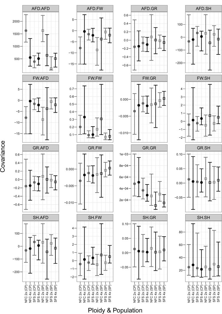
The G matrices for the both methods of generating priors are shown together. Traits are abbreviated as follows: average flowering date (AFD), flower width (FW), growth rate (GR), and scape height (SH). We used the posterior distributions to calculate 95% credible intervals for each trait covariance. This plot shows the median of the posterior as dots (combined prior) or squares (separate prior), and the credible interval as error bars. Only the variance in average flowering date was found to be different between ploidies, and only in the NFC population.

Inspection of the posterior distributions revealed that all eigenvalues for both populations and both ploidies were significantly different than zero, indicating that the dimensionality of G was the same as the number of traits included in the analysis, i.e. four (Figure 3). The eigenvalues and eigenvectors were unaffected by the prior. In general, the eigenvectors were very similar across ploidies and populations; each being approximately a unit vector in the direction of one of the trait axes, suggesting a lack of genetic correlations (Figure 3). The eigenvalues were however somewhat divergent. The first eigenvalue was the most different between ploidies and populations, and was significantly larger in the NFC diploids than either ploidy from the SFS population though indistinguishable from the NFC tetraploids. The second, third and fourth eigenvalues were very similar across both populations and ploidies.

Figure 3. Eigenvalues & Vectors.

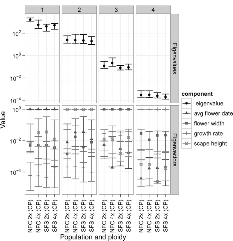
Using the posterior distributions, we calculated 95% credible intervals for each eigenvalue and eigenvector for each population and ploidy. This plot shows the mode of the posterior as dots, and the credible interval as error bars. Due to the orthogonal nature of eigenvectors, we took the absolute value of the individual eigenvector components before plotting.

Discussion

Our results demonstrate that polyploidization can cause immediate phenotypic differentiation and result in significant changes in the structure of the phenotypic covariance matrix. Specifically, trait by trait comparisons across ploidies revealed significant differentiation for several ecologically relevant traits such as flowering phenology and flower size. Additional bootstrap, MANOVA Jackknife, and Flury Hierarchy analyses demonstrated that the P matrices also differed across ploidies. In contrast, although we found significant genetic variation in all traits, virtually no significant differences in the G matrix were identified across ploidy.

We found patterns of phenotypic differentiation consistent with predictions based on increased polyploid cell size (Otto 2007). The tetraploid plants grew slower, flowered somewhat later, and had larger flowers, as has been found in other studies (Otto and Whitton 2000). These patterns of phenotypic differentiation were consistent across population of origin. Our results also demonstrated several significant differences in the P matrix across ploidy. Specifically, in both populations, tetraploids displayed significantly less phenotypic variation than the diploids for four of the seven traits in the analysis, and no difference in variation for the other three traits. The generality of this result is unknown due to very few published comparisons of overall variation in morphologic traits across ploidies, and in studies that do at least publish trait ranges (Borrill and Lindner 1971; Husband and Schemske 2000) there is no clear consensus. The Flury Hierarchy analysis also revealed that the P matrices were indeed different across ploidies in both populations, with the most likely model being that the P matrices share only some of their principal components across cytotypes. It is therefore not surprising that the MANOVA jackknife analysis also revealed a significant affect of ploidy.

In contrast to the P matrix, our analyses of the G matrices did not reveal important impacts of polyploidization. Though it should be noted that in this study (like all studies where P and G are estimated) there is more power to detect differences in P than G. Specifically, although our analyses revealed significant genetic variation for all traits and populations (Figure 3) we were unable to identify any significant differences in genetic variation across ploidies by comparing entries within the G matrices. This was true for both methods of generating priors. Since using different priors to estimate the G matrices is biased towards finding the G matrices to be different, our finding that they are indistinguishable may be conservative. Somewhat surprisingly, our analysis also revealed that most genetic covariances were statistically indistinguishable from zero. This may indicate that either the traits examined in this study are truly genetically independent and not statistically associated, or that our sample sizes were not large enough to detect the statistical associations, or some combination thereof. Since the posterior modes of the covariances were very small in magnitude, and the posterior distributions nearly symmetrical about zero, it is most likely that the true genetic covariances are nearly zero. However, we are unable to rule out the possibility that our failure to detect differences in the G matrices is due to a lack of power. Additionally, if the dominance variance is not small relative to the additive variance as we have assumed, our estimates of the tetraploid G matrices may be inflated.

Given that we found differences between ploidies in the P matrices but not the G matrices, there are a limited number of explanations under the standard model of phenotypic variation, V_P = V_G + V_E + V_{G × E}. First, tetraploids could vary in different ways in response to the environment, (changes in V_E). Indeed, recent studies have documented changes in phenotype in newly formed polyploids due to dosage and epigenetic effects (Shaked et al. 2001; Liu and Wendel 2003; Comai 2005; Chen and Ni 2006; Gaeta et al. 2007). However, the majority of these studies are in allopolyploids, and epigenetic effects in autopolyploids are largely undocumented (Comai 2005). Second, tetraploids could vary in genotype by environment variance (V_{G × E}). Because all the plants in this study were grown in a common garden, we were unable to test this hypothesis, but at least one previous study using allopolyploids did document altered genotype by environment interactions (Schranz and Osborn 2004). Finally, because the genetic variance (V_G) can be separated into additive variance (the G matrix), dominance variance, and epistatic variance, changes in V_P could be due to changes in the dominance or epistatic components of V_G. Again, little is known about how autopolyploidy may alter these variance components. Currently, insufficient evidence exists to speculate on which of these alternatives is most likely.

Because we have generated synthetic autotetraploids from a species which has naturally occurring and well-studied diploids and autotetraploids, we are able to compare and contrast differences we have observed in our synthetic polyploids with those observed in the wild. An interesting contrast between our results and those observed in natural populations occurs with respect to phenology. Specifically, within two well-studied natural populations of sympatric diploid and tetraploid plants growing along the Main Fork Salmon River (MFS) and the Lower Selway River (LS), the tetraploid plants flower significantly earlier than the diploids (Nuismer and Cunningham 2005; Thompson and Merg 2008), whereas our synthetic SFS neotetraploids flower later than their diploid progenitors. Due to the reduced fitness of intercytotype matings, selection should favor disparate flowering times, so as to increase the amount of assortative mating that occurs within cytotypes (Nuismer and Cunningham 2005). However, the observation that the neotetraploids initially flower later than the diploids suggests that evolving the pattern of phenological divergence observed at these sites would require crossing a significant adaptive valley. Thus, a more likely explanation for observed patterns of phenological divergence may be that diploids and tetraploids diverged in allopatry and current patterns of sympatry are the result of post-divergence dispersal. This explanation is consistent with molecular studies suggesting that some tetraploids at the MFS site did not originate from the sympatric diploids (Segraves et al. 1999).

There is evidence in the literature that the phenotypic effect of a polyploidization may depend strongly on population of origin (Segraves and Thompson 1999). However, our study offers little evidence to corroborate this observation. The expected phenotypic consequences of polyploidy, including slower growth and larger flower size are consistent across populations, as is later flowering, though average flowering date was only significantly different between cytotypes in the SFS population. Since Segraves and Thompson studied long established polyploid populations, the likely explanation for the apparent discrepancy between our results and theirs is simply that while the immediate effects of polyploidy may be similar, the path that evolution takes after the polyploidization event varies considerably and may be heavily influenced by spatially variable patterns of selection (Thompson 1994).

Recent research has focused on the immediate genetic consequences of polyploidy, with studies finding evidence of epigenetic effects, gene silencing, and rapid changes in phenotype (Shaked et al. 2001; Gaeta et al. 2007; Buggs et al. 2009; Flagel and Wendel 2009). However, because the majority of this research is in allopolyploid species, it is difficult to separate the effects of polyploidy per se from the effects of a hybrid genome (Parisod et al. 2010). Lacking broad empirical predictions for autopolyploids, we must turn to theory in order to hypothesize how polyploidy affects patterns of genetic variance, and thus the rate and direction of evolution.

Several authors have attempted to predict the effects of polyploidy on the course of evolution using theory. For one locus selection models where the phenotypes of autotetraploids have the same range as diploids, autotetraploids will always have a smaller response to selection than a comparable diploid, suggesting that autotetraploids evolve slower than diploids (Haldane 1927; Hill 1970). However, Otto and Whitton (2000) convincingly argued that the overall rate of adaptive evolution depends not just on the response to selection, but also the frequency with which beneficial mutations arise. Because tetraploids carry more alleles, they have a greater chance of carrying new beneficial alleles. Furthermore, an additional source of potentially beneficial alleles for tetraploids comes from their greater capacity to mask deleterious alleles, which may become beneficial when the environment changes. Finally, Otto and Whitton (2000) concluded that the comparative rates of adaptive evolution depend on the mode of reproduction, the population size, and dominance coefficients of new beneficial alleles. Using a quantitative genetics framework, Ehlke and Hill (1988) showed that differences between the parent-offspring covariances and the rate of adaptive evolution between diploids and autotetraploids depends on the presence of nonadditive genetic effects. Our analysis (Appendix 1) similarly showed that any differences in G between ploidies are due to pleiotropic effects. Thus, models that restrict polyploids to the phenotypic range of diploids predict that tetraploids will have a reduced response to selection. In contrast, without such restrictions on phenotypic range, models predict that tetraploids may exhibit increased or decreased genetic variance, and thus potentially a more rapid response to selection. Our data are consistent with autotetraploids having equivalent genetic variance to diploids, and therefore a similar response to selection. However, further empirical studies will be necessary to illuminate broad patterns.

In summary, our results demonstrate that autopolyploidy can result in immediate phenotypic differentiation of individual traits and also cause potentially important shifts in the structure of the phenotypic covariance matrix. Combined, this immediate phenotypic differentiation and the potential for polyploids to experience divergent selection along novel lines of phenotypic variation may allow polyploids to diversify sufficiently rapidly for them to escape the hurdles imposed by MCE.

References

- Arumuganathan K, Earle ED. Estimation of nuclear DNA content of plants by flow cytometry. Plant Molecular BIology Reporter. 1991;9:229–233. [Google Scholar]
- Begin M, Roff DA. The constancy of the g matrix through species divergence and the effects of quantitative genetic constraints on phenotypic evolution: A case study in crickets. Evolution. 2003;57:1107–1120. doi: 10.1111/j.0014-3820.2003.tb00320.x. [DOI] [PubMed] [Google Scholar]
- Borrill M, Lindner R. Diploid-tetraploid sympatry in dactylis (gramineae) New Phytologist. 1971;70:1111–1124. [Google Scholar]
- Buggs RJA, Doust AN, Tate JA, Koh J, Soltis K, Feltus FA, Paterson AH, Soltis PS, Soltis DE. Gene loss and silencing in tragopogon miscellus (asteraceae): Comparison of natural and synthetic allotetraploids. Heredity. 2009;103:73–81. doi: 10.1038/hdy.2009.24. [DOI] [PubMed] [Google Scholar]
- Buggs RJA, Pannell JR. Ecological differentiation and diploid superiority across a moving ploidy contact zone. Evolution. 2007;61:125–140. doi: 10.1111/j.1558-5646.2007.00010.x. [DOI] [PubMed] [Google Scholar]
- Burton TL, Husband BC. Fitness differences among diploids, tetraploids, and their triploid progeny in chamerion angustifolium: Mechanisms of inviability and implications for polyploid evolution. Evolution. 2000;54:1182–1191. doi: 10.1111/j.0014-3820.2000.tb00553.x. [DOI] [PubMed] [Google Scholar]
- Chen ZJ, Ni ZF. Mechanisms of genomic rearrangements and gene expression changes in plant polyploids. Bioessays. 2006;28:240–252. doi: 10.1002/bies.20374. [DOI] [PMC free article] [PubMed] [Google Scholar]
- Comai L. The advantages and disadvantages of being polyploid. Nat Rev Genet. 2005;6:836–846. doi: 10.1038/nrg1711. [DOI] [PubMed] [Google Scholar]
- Ehlke NJ, Hill RR. Quantitative gentics of allotetraploid and autotetraploid populations. Genome. 1988;30:63–69. [Google Scholar]
- Felber F. Establishment of a tetraploid cytotype in a diploid population: Effect of relative fitness of the cytotypes. Journal of Evolutionary Biology. 1991;4:195–207. [Google Scholar]
- Flagel LE, Wendel JF. Gene duplication and evolutionary novelty in plants. New Phytologist. 2009;183:557–564. doi: 10.1111/j.1469-8137.2009.02923.x. [DOI] [PubMed] [Google Scholar]
- Gaeta RT, Pires JC, Iniguez-Luy F, Leon E, Osborn TC. Genomic changes in resynthesized brassica napus and their effect on gene expression and phenotype. Plant Cell. 2007;19:3403–3417. doi: 10.1105/tpc.107.054346. [DOI] [PMC free article] [PubMed] [Google Scholar]
- Gallais A. Quantitiative genetics and breeding methods in autopolyploid plants. Institut National de la Recherche Agronomique; Paris: 2003. [Google Scholar]
- Hadfield J. Mcmc methods for mulit-response generalised linear mixed models: The mcmcglmm r package. Journal of Statistical Software. 2010;33:1–22. [Google Scholar]
- Haldane JBS. A mathematical theory of natural and artificial selection. Part iii. Proceedings of the Cambridge Philosophical Society. 1927;23:363–372. [Google Scholar]
- Haldane JBS. Theoretical genetics of autopolyploids. Journal of Genetics. 1930;22:359–372. [Google Scholar]
- Halverson K, Heard S, Nason J, Stireman J. Differential attack on diploid, tetraploid, and hexaploid solidago altissima l. By five insect gallmakers. Oecologia. 2008;154:755–761. doi: 10.1007/s00442-007-0863-3. [DOI] [PubMed] [Google Scholar]
- Hill RR. Selection in autotetraploids. TAG Theoretical and Applied Genetics. 1970;41:181–186. doi: 10.1007/BF00277621. [DOI] [PubMed] [Google Scholar]
- Hine E, Blows MW. Determining the effective dimensionality of the genetic variance-covariance matrix. Genetics. 2006;173:1135–1144. doi: 10.1534/genetics.105.054627. [DOI] [PMC free article] [PubMed] [Google Scholar]
- Husband BC, Ozimec B, Martin SL, Pollock L. Mating consequences of polyploid evolution in flowering plants: Current trends and insights from synthetic polyploids. International Journal of Plant Sciences. 2008;169:195–206. [Google Scholar]
- Husband BC, Sabara HA. Reproductive isolation between autotetraploids and their diploid progenitors in fireweed, chamerion angustifolium (onagraceae) New Phytologist. 2004;161:703–713. doi: 10.1046/j.1469-8137.2004.00998.x. [DOI] [PubMed] [Google Scholar]
- Husband BC, Schemske DW. Ecological mechanisms of reproductive isolation between diploid and tetraploid chamerion angustifolium. Journal of Ecology. 2000;88:689–701. [Google Scholar]
- Lande R. Quantitative genetic analysis of multivariate evolution, applied to brain: Body size allometry. Evolution. 1979;33:402–416. doi: 10.1111/j.1558-5646.1979.tb04694.x. [DOI] [PubMed] [Google Scholar]
- Levin DA. Minority cytotype exclusion in local plant populations. Taxon. 1975;24:35–43. [Google Scholar]
- Levin DA. Polyploidy and novelty in flowering plants. American Naturalist. 1983;122:1–25. [Google Scholar]
- Liu B, Wendel JF. Epigenetic phenomena and the evolution of plant allopolyploids. Molecular Phylogenetics and Evolution. 2003;29:365–379. doi: 10.1016/s1055-7903(03)00213-6. [DOI] [PubMed] [Google Scholar]
- Lynch M, Walsh B. Genetics and analysis of quantitative traits. Sinauer Associates, Inc.; Sunderland, MA: 1998. [Google Scholar]
- Nuismer SL, Cunningham BM. Selection for phenotypic divergence between diploid and autotetraploid heuchera grossulariifolia. Evolution. 2005;59:1928–1935. [PubMed] [Google Scholar]
- Nuismer SL, Ridenhour BJ. The contribution of parasitism to selection on floral traits in heuchera grossulariifolia. Journal of Evolutionary Biology. 2008;21:958–965. doi: 10.1111/j.1420-9101.2008.01551.x. [DOI] [PubMed] [Google Scholar]
- Nuismer SL, Thompson JN. Plant polyploidy and non-uniform effects on insect herbivores. Proceedings of the Royal Society B: Biological Sciences. 2001;268:1937–1940. doi: 10.1098/rspb.2001.1760. [DOI] [PMC free article] [PubMed] [Google Scholar]
- Osborn TC, Pires CJ, Birchler JA, Auger DL, Jeffery Chen Z, Lee HS, Comai L, Madlung A, Doerge RW, Colot V, Martienssen RA. Understanding mechanisms of novel gene expression in polyploids. Trends in Genetics. 2003;19:141–147. doi: 10.1016/s0168-9525(03)00015-5. [DOI] [PubMed] [Google Scholar]
- Otto SP. The evolutionary consequences of polyploidy. Cell. 2007;131:452–462. doi: 10.1016/j.cell.2007.10.022. [DOI] [PubMed] [Google Scholar]
- Otto S, Whitton PJ. Polyploid incidence and evolution. Annu Rev Genet. 2000;34:401–437. doi: 10.1146/annurev.genet.34.1.401. [DOI] [PubMed] [Google Scholar]
- Parisod C, Holderegger R, Brochmann C. Evolutionary consequences of autopolyploidy. New Phytologist. 2010;186:5–17. doi: 10.1111/j.1469-8137.2009.03142.x. [DOI] [PubMed] [Google Scholar]
- Phillips PC, Arnold SJ. Hierarchical comparison of genetic variance-covariance matrices. I. Using the flury hierarchy. Evolution. 1999;53:1506–1515. doi: 10.1111/j.1558-5646.1999.tb05414.x. [DOI] [PubMed] [Google Scholar]
- R Core Development Team. R: A language and environment for statistical computing. R Foundation for Statistical Computing; Vienna: 2009. [Google Scholar]
- Ramsey J, Schemske DW. Neopolyploidy in flowering plants. Annu Rev Ecol Syst. 2002;33:589–639. [Google Scholar]
- Rasband WS. Imagej. U. S. National Institutes of Health; Bethesda, Maryland: 1997–2009. [Google Scholar]
- Roff D. Comparing gmatrices: A manova approach. Evolution. 2002;56:1286–1291. [PubMed] [Google Scholar]
- Roff DA, Mousseau T. The evolution of the phenotypic covariance matrix: Evidence for selection and drift in melanoplus. Journal of Evolutionary Biology. 2005;18:1104–1114. doi: 10.1111/j.1420-9101.2005.00862.x. [DOI] [PubMed] [Google Scholar]
- Schluter D. Adaptive radiation along genetic lines of least resistance. Evolution. 1996;50:1766–1774. doi: 10.1111/j.1558-5646.1996.tb03563.x. [DOI] [PubMed] [Google Scholar]
- Schranz ME, Osborn TC. De novo variation in life-history traits and responses to growth conditions of resynthesized polyploid brassica napus (brassicaceae) American Journal of Botany. 2004;91:174–183. doi: 10.3732/ajb.91.2.174. [DOI] [PubMed] [Google Scholar]
- Segraves KA, Thompson JN. Plant polyploidy and pollination: Floral traits and insect visits to diploid and tetraploid heuchera grossulariifolia. Evolution. 1999;53:1114–1127. doi: 10.1111/j.1558-5646.1999.tb04526.x. [DOI] [PubMed] [Google Scholar]
- Segraves KA, Thompson JN, Soltis DE, Soltis PS. Multiple origins of polyploidy and the geographic structure of heuchera grossulariifolia. Molecular Ecology. 1999;8:253. [Google Scholar]
- Shaked H, Kashkush K, Ozkan H, Feldman M, Levy AA. Sequence elimination and cytosine methylation are rapid and reproducible responses of the genome to wide hybridization and allopolyploidy in wheat. Plant Cell. 2001;13:1749–1759. doi: 10.1105/TPC.010083. [DOI] [PMC free article] [PubMed] [Google Scholar]
- Sokal RR, Rohlf FJ. Biometry. W.H. Freeman and Company; New York: 1995. [Google Scholar]
- Soltis PS. Ancient and recent polyploidy in angiosperms. New Phytologist. 2005;166:5–8. doi: 10.1111/j.1469-8137.2005.01379.x. [DOI] [PubMed] [Google Scholar]
- Soltis PS, Soltis DE. The role of genetic and genomic attributes in the success of polyploids. Proceedings of the National Academy of Sciences of the United States of America. 2000;97:7051. doi: 10.1073/pnas.97.13.7051. [DOI] [PMC free article] [PubMed] [Google Scholar]
- Steppan SJ. Phylogenetic analysis of phenotypic covariance structure. 2. Reconstructing matrix evolution. Evolution. 1997;51:587–594. doi: 10.1111/j.1558-5646.1997.tb02445.x. [DOI] [PubMed] [Google Scholar]
- Steppan SJ, Phillips PC, Houle D. Comparative quantitative genetics: Evolution of the g matrix. Trends in Ecology & Evolution. 2002;17:320–327. [Google Scholar]
- Thompson JN. The coevolutionary process. The University of Chicago Press; Chicago: 1994. [Google Scholar]
- Thompson JN, Cunningham BM, Segraves KA, Althoff DM, Wagner D. Plant polyploidy and insect/plant interactions. American Naturalist. 1997;150:730–743. doi: 10.1086/286091. [DOI] [PubMed] [Google Scholar]
- Thompson JN, Merg KF. Evolution of polyploidy and the diversification of plant-pollinator interactions. Ecology. 2008;89:2197–2206. doi: 10.1890/07-1432.1. [DOI] [PubMed] [Google Scholar]
- Wolf PG, Soltis DE, Soltis PS. Chloroplast-DNA and allozymic variation in diploid and autotetraploid heuchera grossulariifolia (saxifragaceae) American Journal of Botany. 1990;77:232–244. doi: 10.1002/j.1537-2197.1990.tb13549.x. [DOI] [PubMed] [Google Scholar]
Associated Data
This section collects any data citations, data availability statements, or supplementary materials included in this article.