Optimally-Discriminative Voxel-Based Morphometry significantly increases the ability to detect group differences in Schizophrenia, Mild Cognitive Impairment, and Alzheimer’s Disease

Abstract

Optimally-Discriminative Voxel-Based Analysis (ODVBA) (Zhang and Davatzikos, 2011) is a recently-developed and validated framework of voxel-based group analysis, which transcends limitations of traditional Gaussian smoothing in forms of analysis such as the General Linear Model (GLM). ODVBA estimates the optimal non-stationary and anisotropic filtering of the data prior to statistical analyses to maximize the ability to detect group differences. In this paper, we extensively evaluate ODVBA to three sets of previously published data from studies in schizophrenia, mild cognitive impairment, and Alzheimer’s disease, and evaluate the regions of structural difference identified by ODVBA versus standard Gaussian smoothing and other related methods. The experimental results suggest that ODVBA is considerably more sensitive in detecting group differences, presumably because of its ability to adapt the regional filtering to the underlying extent and shape of a group difference, thereby maximizing the ability to detect such difference. Although there is no gold standard in these clinical studies, ODVBA demonstrated highest significance in group differences within the identified voxels. In terms of spatial extent of detected area, agreement of anatomical boundary, and classification, it performed better than other tested voxel-based methods and competitively with the cluster enhancing methods.

1. Introduction

Voxel-Based Morphometry (VBM) (Ashburner et al., 2000, Good et al., 2001, Davatzikos et al., 2001a), which analyzes the whole brain in an automated manner, has been developed to characterize brain changes on structural Magnetic Resonance Imaging (MRI), without defining labor-intensive and potentially-biased regions of interest (ROI). To date, VBM has been widely applied in investigating different types of brain disorders, including Schizophrenia, Mild Cognitive Impairment (MCI), and Alzheimer’s Disease (AD). However, in conventional VBM methods which implement the General Linear Model (GLM) (Friston et al., 1995), integrating imaging signals from a region using Gaussian pre-smoothing proves challenging due to difficulty in selecting the appropriate kernel size (Jones et al., 2004, Zhang et al., 2008). If the kernel is too small for the task, statistical power is lost and large numbers of false negatives are bound to confound the analysis; if the kernel is too large, the extensive smoothing will reduce both sensitivity and spatial resolution, typically blurring unrelated structural regions and leading to false positive conclusions about the origin of the structural abnormalities.

Most importantly, Gaussian smoothing will always lack the spatial adaptivity necessary to optimally match image filtering with an underlying (unknown a priori) region of interest. Some spatially adaptive methods have been developed to address this drawback. Davatzikos et al. (Davatzikos et al., 2001b) developed a spatially adaptive filter whose shape changes with the assistance of a pre-defined atlas (also known as ROIs). This method would be effective if true group abnormalities coincide with these pre-defined anatomical boundaries, but this is not always the case. More generally in image processing, full data-driven spatially adaptive methods which do not require ROI’s have been pursued in various contexts. Perona and Malik (Perona and Malik, 1990) developed the Anisotropic Diffusion scheme which removes noise using gradient information while preserving object boundaries. This method was subsequently extended (Gerig et al., 1992) into MRI applications. Polzehl and Spokoiny (Polzehl and Spokoiny, 2000, 2006) proposed a local density estimation-based method for adaptive weights smoothing, named Propagation-Separation (PS), which preserves spatial extent and shapes of the activated regions in images having large homogeneous areas and sharp discontinuities. This method has subsequently been applied to fMRI activation detection (Tabelow et al., 2006). A wavelet-based denoising method was proposed by Pizurica et al. (Pizurica et al., 2003) to adaptively preserve useful image features against the degree of noise reduction by using a wavelet domain indicator of local spatial activity. However, all the above methods work on each single subject separately; that is, they do not take into account the population information, i.e., discriminative information, in a two-group comparison analysis. Hence, the selected filter is adaptive to each subject’s morphological or functional characteristics, but may not be optimal for the purpose of performing group comparisons.

Optimally-Discriminative Voxel-Based Analysis (ODVBA) (Zhang and Davatzikos, 2011) is a recently-developed framework of group analysis utilizing a new spatially adaptive scheme in order to determine group differences with maximal sensitivity. A regional discriminative analysis, with non-negativity constraints on the respective weight coefficients, is conducted in a spatial neighborhood around each voxel to determine the optimal coefficients that best highlight the difference between two groups in that neighborhood. The components of the resultant discriminatory direction can be viewed as weights of a local spatial filter, which is optimally designed to highlight group differences. The weights determined for a given voxel from all the regional analyses it belongs to are combined into a map representing statistically significant voxel-wise group differences, using permutation tests. Adaptive smoothing is inherent in ODVBA, and is similar in concept to the nonstationarity adjustment in smoothness (Hayasaka and Nichols, 2003, Hayasaka et al, 2004, Salimi-Khorshidi et al, 2009) utilized in cluster-level statistical inference studies. ODVBA has been evaluated (Zhang and Davatzikos, 2011) by using both simulated and real data and has been found to precisely identify the shape and location of group differences with high sensitivity and specificity.

In this paper, we apply ODVBA to three previously published studies in which the traditional Gaussian smoothing plus GLM was used. In addition, we compare ODVBA to not only GLM but also two other spatially adaptive smoothing methods: PS (Polzehl and Spokoiny, 2000, 2006) and wavelet denosing (WL) (Pizurica et al., 2003), and two versions of the newly-proposed cluster enhancing method, Threshold-Free Cluster Enhancement (TFCE): the original GLM-based TFCE (G-TFCE) (Smith and Nichols, 2009), and an ODVBA-based TFCE (O-TFCE). The three published studies used for this group comparison include 1) a sample of well-characterized patients with schizophrenia and matched controls (Davatzikos et al., 2005). 2) Early-stage MCI patients and the normal controls (Davatzikos et al., 2008), and 3) MCI patients who convert to AD and MCI patients who remain stable(Misra et al., 2009).

2 Methods

2.1 Participants and Imaging protocol

The details on participants’ information and MRI acquisition can be found in (Davatzikos et al., 2005, Davatzikos et al., 2008, Misra et al., 2009). Here, we only provide the basic information of subjects.

• Dataset1: Sixty-nine patients (46 men and 23 women) (Davatzikos et al., 2005) with schizophrenia and seventy-nine controls (41 men 38 women) were involved in the study.

• Dataset2: Thirty older adults (Davatzikos et al., 2008) including 15 subjects with MCI and 15 normal controls were examined in the current study.

• Dataset3: One hundred subjects with MCI were randomly selected from the data used in (Misra et al., 2009). 50 of these subjects had undergone conversion to AD. The remaining 50 are non-converters.

2.2 Image processing

A standard image pre-processing protocol described in (Goldszal et al., 1998) was used in all three parent studies. The result was a RAVENS map, reflecting regional volumetrics (Goldszal et al., 1998; Davatzikos et al., 2001; Shen and Davatzikos, 2002), akin to what was typically used in the “modulated” VBM analysis (Davatzkos et al., 2001a, Good et al., 2001, Ashburner et al., 2003). RAVENS maps quantify the regional distribution of gray matter (GM), white matter (WM), and cerebrospinal fluid (CSF), since one RAVENS map is formed for each tissue type. In this paper, we investigate group differences of GM RAVENS maps.

2.3 Statistical analysis using ODVBA

Group comparisons were performed via voxel-based statistical analysis of RAVENS maps by using ODVBA (Zhang and Davatzikos, 2011). The main premise of ODVBA is that it uses a machine learning paradigm to effectively apply a form of matched filtering, to optimally detect a group difference. Since the shape of the target region of group difference is not known, regional discriminative analyses are used to identify voxels displaying the most significant differences. In addition to potentially improving sensitivity of detection of a structural or functional signal, this approach was shown in both the simulated data and the real world data (Zhang and Davatzikos 2011) to better delineate the region of abnormality, in contrast with conventional smoothing approaches that blur through boundaries and dilute the signal from regions of interest with signal from regions that do not display a group difference.

ODVBA works in three stages:

1. Regional nonnegative discriminative projection: regional discriminative analysis, restricted by appropriate nonnegativity constraints on the coefficients which various voxels have in the discriminating vector, is applied to a spatial neighborhood around each voxel. Specifically, the goal of the regional analysis is not simply to find the coefficients which can distinguish the two groups, but also requires those coefficients relate to the underlying group difference, instead of merely providing some features that happen to separate two groups well. The analysis can result in obtaining parts-based representation of local volumes (neighborhood), as only the elements which make large contributions for discrimination will be highlighted. The left part of Figure 1 illustrates the idea. In neighborhood I, only area within underlying structural changes is highlighted with high values of weights. In neighborhood II, no voxels are assigned high weights since no targeting regions are involved in that neighborhood.

   In particular, for each given voxel x in the volume X (the neighborhood defined by ||x − x_i|| < ζ), ODVBA gets a k dimensional subvolume vector: θ⃗ = [x, x₁, ···, x_k−1]T, where x₁, ···, x_k−1 are the k − 1 neighbors of x, and then it constructs a learning set Θ = [θ⃗₁, ···, θ⃗_N]^T from N subjects of two different groups. ODVBA expects to find a nonnegative vector w to describe the contributions of elements in θ⃗ for classification. Hence, the objective function formulated with nonnegative quadratic programming is defined as follows:

   $$J(\text{w})=\underset{\overrightarrow{w}}{min}{\overrightarrow{w}}^{T}A\overrightarrow{w}-\mu {\overrightarrow{e}}^T\overrightarrow{w},s.t.{(\overrightarrow{w})}_i\ge 0$$ (1)
   where, A = γS_W − S_B +((|λ_min| + τ)I); $S_W={\sum }_{i=1}^2{\sum }_{\overrightarrow{\theta }\in C_i}\left(\overrightarrow{\theta }-{\overrightarrow{m}}_i\right){\left(\overrightarrow{\theta }-{\overrightarrow{m}}_i\right)}^T$; C_i means the i^th group; m⃗_i = 1/N_i Σ_{θ⃗ ∈Ci} θ⃗; N_i denotes the number of samples in C_i; γ is the tuning parameter; S_B = (m⃗₁ − m⃗₂)(m⃗₁ − m⃗₂ )^T; |λ_min| is the absolute of the smallest eigenvalue of γS_W − S_B ; 0 < τ ≪ 1 acts as the regularization parameter; I is the identity matrix; e⃗ is the vector with all ones; μ is the balance parameter. w⃗ is estimated by multiplicative updates (Zhang and Davatzikos, 2011) which iteratively minimize the objective function:

   $${(\overrightarrow{w})}_i\leftarrow \left(\frac{{\left(\mu {\overrightarrow{e}}^T\right)}_i+\sqrt{{{\left(\mu {\overrightarrow{e}}^T\right)}_i}^2+16{\left(A^{+}\overrightarrow{w}\right)}_i{\left(A^{-}\overrightarrow{w}\right)}_i}}{4{\left(A^{+}\overrightarrow{w}\right)}_i}\right){(\overrightarrow{w})}_i,$$ (2)

   where i =1, ···, k; A⁺ and A⁻ are two nonnegative matrices, defined as follows: A⁺_ij = A_ij, if A_ij > 0; otherwise 0. A⁻_ij = |A_ij|, if A_ij < 0; otherwise 0.

2. Determining each voxel’s statistic: Since each voxel belongs to a large number of neighborhoods, each centered on one of its neighboring voxels, the group difference at each voxel is determined by summing up contributions from all neighborhoods to which it participates. As shown in the middle part of Figure 1, the voxel x_a and voxel x_b have their own participating neighborhoods respectively. Because the coefficients obtained from the first stage are nonnegative, the possible cancelations between negative and positive loadings are avoided.

   Specifically, the statistical value of x is defined by summing up contributions from all neighborhoods to which it participates:

   $$S_x=\sum _{\mathbb{N}\in \mathrm{\Delta }}{\delta }_{\mathbb{N}}{\left({\overrightarrow{w}}_{\mathbb{N}}\right)}_i,i\in \{1,\dots ,k\},$$ (3)

   where, w⃗_ℕ denotes the coefficients corresponding to voxels in neighborhood ℕ, Δ ={ℕ|x ∈ ℕ}, (w⃗_ℕ)_i denotes that x is the i^th element in ℕ, and δ_ℕ denotes the discrimination degree (Zhang and Davatzikos 2011).

3. Permutation tests: Permutation tests (Holmes et al., 1996, Nichols et al., 2002) are used to obtain the statistical significance (p values) of the resulting ODVBA maps, assuming that the null hypothesis is that there is no difference between the two groups. We randomly assign group labels to each subject, and then recalculate the statistic as described in Equation 3 for each voxel for N_p times. Let S₀ denote the statistic value obtained under the initial class labels, and S_i, i =1, ···, N_p, denote the ones obtained by relabeling. The p value for the given voxel (illustrated in the right part of Figure 1) is the proportion of the permutation distribution ( S₀, ···, S_NP) greater than or equal to S₀.

   The parameters mentioned above are set as same as those used on the real data in the paper (Zhang and Davatzikos, 2011): ζ =15, μ =1, γ =10⁻⁵, τ =10⁻⁵. However we increased the number of permutations to N_p =5000 for all three studies in this paper. As described in (Zhang and Davatzikos, 2011), an important character of ODVBA is that it has stable performance with varying smoothing kernel size. Here, we evaluate this point by studying the number of detected significant voxels versus different kernel size (the parameter ζ). The significant voxels were defined as those with the unadjusted p value below a specified threshold. The results shown in Figure 2 further verified the stability of ODVBA, especially in contrast to GLM in which Gaussian smoothing is employed. More discussions on evaluation of other methods in Figure 2 can be found in Section 2.4.

Figure 1.

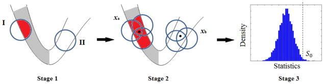
Illustration of the flowchart of ODVBA. ODVBA works in three stages including 1) Regional nonnegative discriminative projection, 2) Determining each voxel’s statistic, and 3) Permutation tests. The gray color in Stage 1 and Stage2 indicates the area with underlying structural changes and the red color indicates the highlighted area via regional discriminative analysis in ODVBA.

Figure 2.

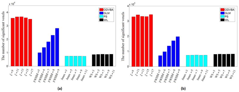
The number of significant voxels versues smoothing kernel sizes. (a) The results are obtained from group comparison between the schizophrenia patients and the normal controls in Dataset 1 where the voxels are counted if the unadjusted p value<0.001; (b) The results are obtained from group comparison between the MCI-to-AD converters and the non-converters in Dataset 3 where the voxels are counted if the unadjusted p value<0.005. The results from Dataset 2 are not included since GLM, PS, and WL did not have detections for most of kernel sizes, with a reasonable low p value threshold.

2.4 Statistical analysis using the comparative methods

Other than ODVBA, we have also implemented five alternative methods for comparison purpose. They are described as follows.

1. GLM: As reported in the three previously-published studies, the conventional Voxel based Morphometry method -- Gaussian smoothing with 8mm full width at half maximum (FWHM) kernel plus GLM, (Ashburner et al., 2000, Davatzikos et al., 2001a) was re-implemented in this paper. The performances of GLM with different FWHM values are also demonstrated in Figure 2. Obviously, they are sensitive to the kernel sizes.

2. PS: The Propagation-Separation (PS) approach (Polzehl and Spokoiny, 2000, 2006) targets to adaptive weights smoothing based on local nonparametric estimation. This is achieved in an iterative process by extending regions of local homogeneity until the obtained structural information agrees with the previous iteration step. We use the freely available software: http://cran.r-project.org/web/packages/aws/ which is implemented in the R environment. In this software, one important parameter is ladjust which can adjust adaptivity of the method and another important one is hmax which specifies the spatial extent of the smoothness. We performed the grid search for ladjust and hmax according to the methods’ performance on group analysis. We finally use ladjust=1 and hmax=5 because 1) PS achieved stable performance around those values and 2) these values are suggested by the user manual of the software package. We demonstrated the numbers of significant voxel detected by PS with varying smoothing kernel sizes, i.e., hmax in Figure 2. The results provided evidence on the adaptivity of PS since the method demonstrated less sensitive to the size of kernel, compared with Gaussian filter used byGLM.

3. WL: Wavelet (WL) denoising (Pizurica et al., 2003) achieve the spatial adaptivity by using a local spatial activity indicator that is computed from a squared window. We use its publicly available software: http://telin.ugent.be/~sanja/Sanja_files/Software/MRIprogram.zip which is designed by the paper author for MRI applications. The important parameters include the window size (WS) and the multiplication factor (MF) which specifies the signal of interest. We use WS=5 and MF=2, which are the default values in the software package. As well as ODVBA, GLM, and PS, in Figure 2 we reported the performance of WL with varying spatial extents of smooth kernel, i.e., the parameter of WS in the software. The results also reveal the stability of WL with different kernel sizes.

4. G-TFCE: Threshold-Free Cluster Enhancement (TFCE) is a newly-proposed method to enhance cluster-like structures in the map of t values in group analysis, without having to define an initial cluster-forming threshold. In the original method, Gaussian smoothing was conducted to reduce the noise, prior to GLM which produces the group contrasts for the TFCE analysis. We name it as G-TFCE. G-TFCE was implemented using the randomise tool in FMRIB Software Library (http://fsl.fmrib.ox.ac.uk/fsl/fslwiki/). As suggested in (Smith and Nichols, 2009), a small amount of Gaussian smoothing with 4mm FWHM kernel, was conducted in G-TFCE.

5. O-TFCE: Our spatially adaptive smoothing method, ODVBA, was employed to replace Gaussian smoothing, and the TFCE scores are calculated based on the statistic image of ODVBA. We thereby name it O-TFCE.

2.5 Correction and interpretation

In this paper, the p-values obtained by all involved methods are then corrected by the FDR procedure (Nichols et al., 2003, Genovese et al., 2002), which is commonly used in neuroimaging applications to adjust for statistical error emanating from multiple comparisons. The corrected significance maps are partitioned and analyzed according to the automated anatomical labeling (AAL) (Tzourio-Mazoyer et. al., 2002) from Wake Forest University (WFU) Pickatlas package (Maldjian et. al., 2003, 2004). On each anatomical region, we calculated the cluster size, the t statistic (based on means of RAVENS values on the detected area per region), and the Talairach coordinate of the cluster’s center. Finally, we used the significant voxels showing the group differences as the input features for cross-validation classification.

3 Results

In this section, we first introduce the results of ODVBA on the three datasets, and then compare ODVBA’s results to that of the comparative methods.

3.1. Findings of ODVBA

• Dataset1: A widespread pattern of significant GM loss (FDR corrected p<0.01, spatial extent threshold >50) was detected in the comparison between 69 schizophrenia patients and 79 normal controls. They are mainly in 1) frontal area bilaterally including the orbitofrontal cortex, the middle frontal gyrus, the supplementary motor area, the superior frontal gyrus-medial part, the precentral gyrus, the inferior frontal gyrus, and the superior frontal gyrus; 2) temporal area bilaterally including the middle, inferior, and superior temporal gyrus, and the fusiform gyrus; 3) parietal area bilaterally, e.g., the postcentral gyrus, the precuneus, and the inferior parietal gyrus; 4) limbic system bilaterally, e.g., the median cingulate, the anterior cingulate, and the hippocampus, and 5) sub-lobar, e.g., bilateral insular cortex. The full list of regions and the associate statistical information are presented in Table 1, and the representative slices in the sagittal view are shown Figure 3. According to the results shown in Table 1, the left middle temporal gyrus, the right orbitofrontal cortex, and the right middle temporal gyrus demonstrate the three largest regions of atrophy based on their significant voxel numbers.

• Dataset2: MCI subjects presented significant GM atrophy (FDR corrected p<0.05, spatial extent threshold >50) compared to the normal controls mainly in 1) parietal lobe bilaterally including the precuneus, the superior parietal gyrus, the postcentral gyrus, and the inferior parietal gyrus; 2) frontal lobe including the bilateral middle frontal gyrus, the left inferior frontal gyrus, and the left superior frontal gyrus; 3) limbic lobe, e.g., the left hippocampus, the left parahippocampal gyrus, and the left amygdala; 4) temporal lobe including the left middle, inferior, and superior temporal gyrus, and the left fusiform gyrus; 5) left insular cortex. For detail, see Table 2 and Figure 4. The left middle frontal gyrus, the left precuneus, and the right precuneus demonstrate the largest regions of atrophy based on their significant voxel numbers.

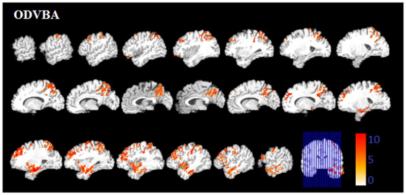
• Dataset3: The comparison between baseline data of MCI-to-AD converters and non-converters revealed significant low (FDR corrected p<0.05, spatial extent threshold >50) GM value of converters in (Table 3 and Figure 5) 1) temporal lobe bilaterally including the superior, middle and inferior temporal gyrus, the temporal pole, and the fusiform gyrus; 2) limbic lobe bilaterally including the parahippocampal gyrus, the hippocampus, and the amygdala; 3) frontal area, e.g., the bilateral orbitofrontal cortex, the bilateral straight gyrus, the right rolandic operculum, and the right precentral gyrus; 4) parietal lobe including the bilateral precuneus, the bilateral angular, the right postcentreal gyrus, and the right supramarginal gyrus; and 5) some sub-lobar regions bilaterally including the insular cortex, the putamen, and the heschl gyrus. The top three largest regions are the right middle temporal gyrus, the left middle temporal gyrus, and the right superior temporal gyrus.

Table 1.

Statistical results of ODVBA on the group comparison between Schizophrenia patients and normal controls.

Lobe	Region	Side	Talairach coordinates			Number of Voxels	t values
			x	y	z
Frontal Lobe	Orbitofrontal Cortex	R	41.58	32.52	−10.04	1712	6.87
	Middle Frontal Gyrus	L	−35.64	32.66	31.53	1220	8.39
	Superior Frontal Gyrus	R	21.78	19.92	48.75	1189	8.68
	Superior Frontal Gyrus	L	−17.82	27.3	41.01	1105	9.21
	Orbitofrontal Cortex	L	−33.66	30.41	−13.3	1039	6.45
	Middle Frontal Gyrus	R	33.66	9.96	43.72	1016	8.86
	Superior Frontal Gyrus, medial	L	−5.94	51.48	19.53	928	7.29
	Supplementary Motor Area	L	−5.94	6.54	53.1	835	8.31
	Supplementary motor area	R	7.92	6.63	54.94	794	6.93
	Inferior Frontal Gyrus	L	−45.54	27.86	13.34	756	6.03
	Precentral Gyrus	L	−31.68	−9.05	52.04	688	7.92
	Precentral Gyrus	R	41.58	−7.48	44.59	681	7.85
	Superior Frontal Gyrus, medial	R	7.92	33.3	44.39	596	7.28
	Inferior Frontal Gyrus	R	49.5	35.24	5.61	479	6.14
	Paracentral Lobule	L	−5.94	−22.06	63.74	305	7.69
	Supramarginal Gyrus	R	45.54	−29.07	40.14	241	4.37
	Straight Gyrus	L	−3.96	32.1	−18.43	234	5.92
	Straight Gyrus	R	5.94	28.14	−19.91	201	5.9
	Rolandic Operculum	R	55.44	−7.2	11.41	139	7
	Rolandic Operculum	L	−43.56	−24.54	14.12	92	6.71
Limbic Lobe	Median Cingulate	R	3.96	7.65	36.46	531	7.17
	Median Cingulate	L	−1.98	−0.01	38.69	378	7.37
	Hippocampus	R	33.66	−19.96	−10.78	266	4.77
	Anterior Cingulate	L	−5.94	44.75	1.45	254	6.51
	Parahippocampal Gyrus	R	29.7	−22.24	−17.39	228	5.51
	Anterior Cingulate	R	5.94	41.52	14.5	207	6.64
	Calcarine Fissure	L	−11.88	−63.39	14.23	181	5.61
	Hippocampus	L	−33.66	−21.9	−10.68	112	4.59
	Calcarine Fissure	R	19.8	−55.82	10.16	94	5.7
Occipital Lobe	Lingual Gyrus	L	21.78	−60.4	−3.71	322	6.46
	Inferior Occipital Gyrus	R	45.54	−74.13	−6.38	220	5.02
	Inferior Occipital Gyrus	L	−49.5	−66.46	−8.45	216	5.8
	Lingual Gyrus	L	−7.92	−62	3.1	154	6.59
	Cuneus	L	−11.88	−60.8	26.99	140	5.56
	Superior Occipital Gyrus	L	−19.8	−64.5	30.86	102	4.32
	Middle Occipital Gyrus	L	−45.54	−71.77	1.91	100	6.19
Parietal Lobe	Precuneus	L	−7.92	−62.19	38.12	709	8.19
	Postcentral Gyrus	R	51.48	−15.6	37.63	695	8.6
	Postcentral Gyrus	L	−47.52	−17.35	41.4	531	8.84
	Inferior Patietal Gyrus	L	−33.66	−40.6	42.56	445	5.99
	Inferior Patietal Gyrus	R	37.62	−42.36	46.33	380	8.38
	Precuneus	R	7.92	−50.29	43.05	330	7.62
	Supramarginal Gyrus	L	−47.52	−31.74	25.54	151	7.77
	Angular Gyrus	R	33.66	−50.38	41.21	83	5.01
Temporal Lobe	Middle Temporal Gyrus	L	−57.42	−34.96	0.07	1834	7.7
	Middle Temporal Gyrus	R	59.4	−33.19	−3.39	1419	9
	Inferior Temporal Gyrus	L	−51.48	−39.68	−16.52	1070	6.51
	Inferior Temporal Gyrus	R	53.46	−39.59	−14.84	1031	6.52
	Superior Temporal Gyrus	L	−51.48	−30.35	14.41	759	7.42
	Fusiform Gyrus	R	33.66	−43.38	−12.97	772	6.52
	Superior Temporal Gyrus	R	57.42	−19.28	2.8	692	6.44
	Fusiform Gyrus	L	−29.7	−28.21	−20.46	605	7.14
	Temporal Pole	R	49.5	18.7	−14.39	269	5.99
Sub-lobar	Insular Cortex	R	33.66	18.96	−9.36	198	6.22
	Insular Cortex	L	−31.68	21.31	−1.07	150	7.28

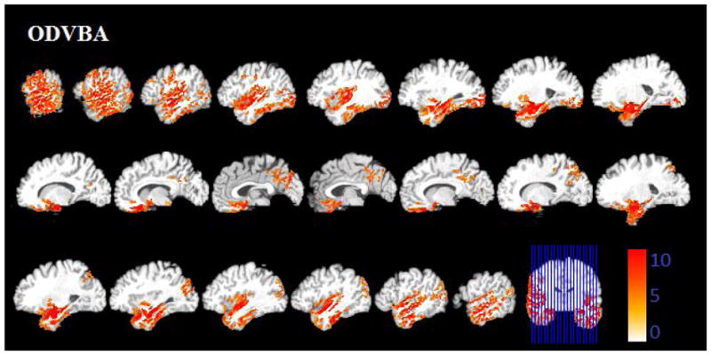
Figure 3.

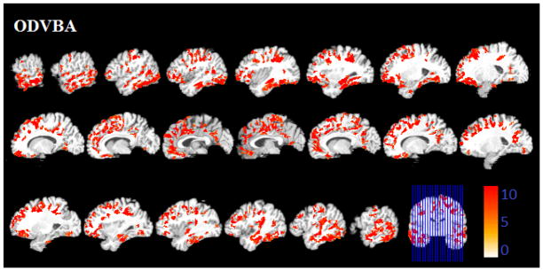
Significant areas of relative decreased gray matter detected by ODVBA in the schizophrenia patients. Images are in radiology convention. Multiple voxel comparisons were corrected using the FDR threshold of p<0.01 and a spatial extent threshold of 50 voxels was applied. Color bar indicates −log (p) value.

Table 2.

Statistical results of ODVBA on the group comparison between MCI patients and normal controls.

Lobe	Region	Side	Talairach coordinates			Number of Voxels	t values
			x	y	z
Frontal Lobe	Middle Frontal Gyrus	L	−35.64	32.74	33.37	953	6.99
	Inferior Frontal Gyrus	L	−47.52	27.86	13.34	627	5.23
	Superior Frontal Gyrus	L	−19.8	46.21	30.85	583	6.66
	Precentral Gyrus	L	−31.68	−8.41	64.9	198	4.23
	Middle Frontal Gyrus	R	35.64	40.41	31.14	169	6.05
Limbic Lobe	Hippocampus	L	−25.74	−16.25	−14.33	251	3.83
	Parahippocampal Gyrus	L	−23.76	−27.79	−12.06	159	3.33
	Amygdala	L	−25.74	−2.77	−16.68	87	3.78
	Median Cingulate	L	−1.98	−38.66	42.47	63	6.15
	Posterior Cingulate	L	−3.96	−47.15	28.15	51	4.99
Parietal Lobe	Precuneus	L	−5.94	−56.01	45.18	729	8.59
	Precuneus	R	5.94	−51.67	54.17	656	5.37
	Supeior Patietal Gyrus	L	−25.74	−53.34	59.78	598	5.35
	Supeior Patietal Gyrus	R	23.76	−55.37	58.04	500	6.88
	Postcentral Gyrus	L	−37.62	−28.7	47.49	390	7.69
	Postcentral Gyrus	R	35.64	−32.48	49.52	290	4.54
	Inferior Patietal Gyrus	L	−37.62	−48.07	48.46	251	4.22
	Inferior Patietal Gyrus	R	39.6	−44.2	48.27	131	5.36
	Angular Gyrus	R	39.6	−57.77	48.95	61	4.74
Temporal Lobe	Middle Temporal Gyrus	L	−57.42	−16.09	−10.97	481	4.5
	Inferior Temporal Gyrus	L	−51.48	−22.4	−20.74	388	5.73
	Superior Temporal Gyrus	L	−45.54	−6.23	−8.09	207	5.52
	Fusiform Gyrus	L	−35.64	−24.25	−18.97	145	3.24
	Temporal Pole	L	−49.5	7.16	−12.13	55	3.94
Sub-lobar	Insular Cortex	L	−39.6	5.56	−5.32	227	3.78

Figure 4.

Significant areas of relative decreased gray matter detected by ODVBA in the MCI patients. Images are in radiology convention. Multiple voxel comparisons were corrected using the FDR threshold of p<0.05 and a spatial extent threshold of 50 voxels was applied. Color bar indicates −log (p) value.

Table 3.

Statistical results of ODVBA on the group comparison between the MCI-to-AD converters and the Non-converters.

Lobe	Region	Side	Talairach coordinates			Number of Voxels	t values
			x	y	z
Frontal Lobe	Orbitofrontal Cortex	L	−13.86	30.08	−20.01	536	4.92
	Rolandic Operculum	R	55.44	−5.35	9.48	520	5.58
	Orbitofrontal Cortex	R	43.56	22.74	−11.23	520	6.01
	Precentral Gyrus	R	53.46	1.83	36.75	369	7.06
	Straight Gyrus	L	−3.96	26.2	−19.81	334	5.83
	Straight Gyrus	R	5.94	28.14	−19.91	307	5.48
	Inferior Frontal Gyrus	R	59.4	13.93	6.67	247	6.31
	Rolandic Operculum	L	−41.58	−18.64	15.67	142	6.72
	Olfactory Cortex	R	13.86	10.87	−15.68	113	5.93
	Olfactory Cortex	L	−1.98	14.83	−14.19	102	3.69
	Precentral Gyrus	L	−37.62	0.36	46.03	65	5.12
Limbic Lobe	Parahippocampal Gyrus	R	25.74	−12.63	−19.55	695	4.45
	Hippocampus	L	−25.74	−18.11	−12.55	645	5.98
	Hippocampus	R	29.7	−18.11	−12.55	618	5.43
	Parahippocampal Gyrus	L	−19.8	−6.99	−23.2	500	4.62
	Amygdala	R	27.72	−0.75	−15.1	237	3.74
	Amygdala	L	−23.76	−2.69	−15	198	4.65
	Median Cingulate	L	−1.98	−38.85	38.79	98	6.00
Occipital Lobe	Middle Occipital Gyrus	L	−33.66	−76.49	24.09	765	7.24
	Inferior Occipital Gyrus	R	39.6	−81.79	−4.31	437	6.51
	Middle Occipital Gyrus	R	37.62	−84.88	11.61	259	7.08
	Lingual Gyrus	R	19.8	−83.73	−4.22	180	6.01
	Cuneus	L	−9.9	−70.21	32.99	145	5.15
	Superior Occipital Gyrus	L	−23.76	−82.02	29.89	141	7.43
	Calcarine Fissure	L	−1.98	−81.01	11.42	138	6.63
	Cuneus	R	9.9	−72.15	33.09	129	7.21
	Inferior Occipital Gyrus	L	−33.66	−81.79	−4.31	79	6.23
Parietal Lobe	Postcentral Gyrus	R	57.42	−10.15	29.98	878	6.27
	Precuneus	L	−5.94	−57.94	45.27	684	7.09
	Supramarginal Gyrus	R	63.36	−23.81	28.82	596	5.72
	Supeior Patietal Gyrus	L	−21.78	−65.42	51.17	364	7.16
	Precuneus	R	3.96	−58.22	39.76	299	6.99
	Angular Gyrus	R	51.48	−58.69	30.57	200	6.99
	Angular Gyrus	L	−43.56	−67.91	40.24	126	5.88
	Inferior Parietal Gyrus	L	−29.7	−69.67	44.02	94	4.31
Temporal Lobe	Middle Temporal Gyrus	R	59.4	−29.39	−5.25	2125	6.50
	Middle Temporal Gyrus	L	−57.42	−27.46	−5.35	2094	6.90
	Superior Temporal Gyrus	R	59.4	−19.19	4.64	2048	6.93
	Inferior Temporal Gyrus	R	53.46	−30.07	−18.68	1557	5.68
	Inferior Temporal Gyrus	L	−49.5	−24.34	−20.64	1399	5.83
	Temporal Pole	R	45.54	10.86	−15.68	1097	5.04
	Fusiform Gyrus	R	35.64	−26.28	−20.55	1044	5.83
	Superior Temporal Gyrus	L	−49.5	−13.56	0.68	922	7.55
	Fusiform Gyrus	L	−29.7	−16.76	−24.39	734	5.11
	Temporal Pole	L	−37.62	8.76	−18.94	725	5.77
Sub-lobar	Insular Cortex	R	43.56	1.85	−1.77	592	5.37
	Insular Cortex	L	−39.6	1.76	−3.45	441	6.48
	Putamen	R	29.7	3.62	−5.22	159	3.81
	Heschl Gyrus	L	−43.56	−17.07	8.22	143	6.14
	Heschl Gyrus	R	49.5	−13.19	8.03	140	5.41
	Putamen	L	−25.74	−0.25	−5.03	118	3.03

Figure 5.

Significant areas of relative decreased gray matter detected by ODVBA in the MCI-to AD converters. Images are in radiology convention. Multiple voxel comparisons were corrected using the FDR threshold of p<0.05 and a spatial extent threshold of 50 voxels was applied. Color bar indicates −log (p) value.

3.2. Comparative results

We focus on the comparisons between results of the involved methods as follows:

1. Spatial extent of the group difference: The spatial maps of GLM, PS, WL, G-TFCE and O-TFCE are shown together in Figures 6, 7, and 8 for three datasets respectively (The results are demonstrated using the same slices with those of ODVBA in Figures 3, 4, and 5. However in Figures 6, 7, and 8, the images are smaller because of space limitation). The numbers of detected significant voxels in each anatomical region obtained from these methods are listed in part of Tables 4, 5, and 6. Note that, for the group analysis between the MCI patients and the normal controls in the Dataset2, GLM, PS, and WL did not produce significant results after FDR correction. We display the total number of significant voxels in a vector for all above methods as well as ODVBA as horizontal bars for three different datasets in Figure 9. According to the results demonstrated from the above tables and figures, it is concluded that ODVBA is generally more sensitive than GLM since it detects more and larger areas of differences. PS and WL produced smaller significant areas than either GLM or ODVBA. The two cluster enhancing methods, i.e., G-TFCE and O-TFCE, produced larger significant areas than the voxel-based statistical methods, and O-TFCE shows stronger statistical power than G-TFCE.

   We highlight the regions which are detected by ODVBA but not by GLM as follows. For the schizophrenia data of Dataset1, ODVBA detected more regions, e.g., the left precentral gyrus, the left paracentral lobule, the left hippocampus, the left superior occipital gyrus, the left middle occipital gyrus, the left supramarginal gyrus, and the right angular gyrus, than GLM. For the group comparison between MCI-to-AD converters and non-converters in Dataset3, ODVBA detected the right precentral gyrus, the right inferior frontal gyrus, the left olfactory cortex, the right lingual gyrus, the left cuneus, the left superior occipital gyrus, the left inferior occipital gyrus, the left superior parietal gyrus, the left angular gyrus, the left inferior parietal gyrus, and the bilateral putamen, none of which were reported by GLM.

2. Significance of the group difference: Based on the detected voxels, we first calculated the means of the GM RAVENS values per region for all subjects in each dataset, since these means reflect the tissue density of the selected area. We subsequently computed the t values, reflecting the significance of group differences based on these means. We list the t values of GLM, PS, WL, G-TFCE and O-TFCE in part of Tables 4–6, as well as ODVBA whose values have been demonstrated in Tables 1–3. We also demonstrate the average t values of anatomical regions in a vector as horizontal bars for all the methods in Figure 10. According to the results collected as above, ODVBA offers the highest t values for the detected area (in each anatomical region), revealing it may have better capability to control false positive errors than other methods, whereas GLM produces the lowest t values. t values of G-TFCE are generally lower than O-TFCE, further suggesting that Gaussian smoothing is inferior to our proposed spatially adaptive method.

3. Spatial agreement between detected regions and underlying tissue boundaries: For comparison of the tested methods by visual inspection, in Figure 11 we focus on a small section of the detected regions near the hippocampus. We see that GLM blurs volumetric measurements from the hippocampus with such measurements from the fusiform gyrus. However, ODVBA delineates a more precise area of significant atrophy, which agrees with GM boundaries, as it should in this experiment that evaluated GM RAVENS maps. Although PS and WL are capable of detecting tissue boundaries, this detection is weak, demonstrating low statistical power. We can also see the G-TFCE (with small Gaussian smoothing) and O-TFCE do not blur volumetric measurements as in GLM, while demonstrating enhanced statistical power.

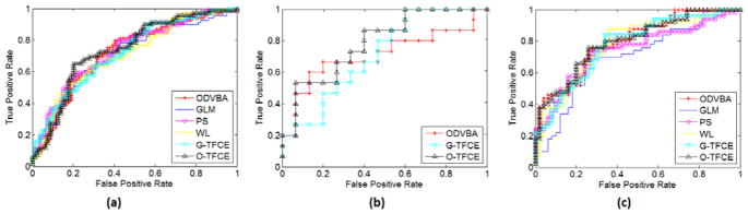
   Furthermore, since we know the underlying anatomy of tissues, we use the metrics of True Positive Rate (TPR) and False Positive Rate (FPR) for evaluation. Here, TPR is the number of significant voxels inside the GM segmentation divided by the total number of voxels in GM. FPR is calculated as the number of significant voxels outside the GM segmentation divided by the total number of voxels in the whole brain volume other than GM. A series of TPR/FPR are produced to build the receiver operating characteristics (ROC) curve, as demonstrated in Figure 12, by varying the significance levels. It is clear that GLM offers a globally worse result than other methods since for any FPR, the corresponding TPR is lower. It is worth noting that PS and WL showed the superior performances on specificity over the other methods in Figure 12(a) in virtue of their spatially adaptive smoothing.

4. Classification accuracy based on detected regions: The significant regions obtained by the six different methods are used as the feature input to classify subjects of the three datasets. Specifically, we first utilized the linear feature transformation method, Principal Component Analysis (PCA) (Jolliffe, 2005), to remove the abundant information in the original features (whose corresponding PCA eigenvalues are zeros), and then employed linear Support Vector Machine (SVM) (Chang and Lin, 2011)as the classifier. The classification was achieved within a Five-fold cross-validation framework. That is, the whole dataset is randomly partitioned into 5 subsets. Of the 5 subsets, a single subset is retained as “testing data” to report the performance, while the remaining 4 subsets are used as “training data” to create the model. In particular, in each fold, ODVBA and the comparative methods are implemented to locate the significant group differences only according to the training data. That means the testing data are not involved in creating the statistical model. Moreover, we conducted the nested cross-validation within the training data for parameter selection, e.g., parameter C in linear SVM. Table 7 lists the average accuracies over cross-validation of six methods. ODVBA achieved a slightly better performance than the other voxel-based methods. However, ODVBA did not perform better than the cluster enhancement methods, G-TFCE and O-TFCE. It is worth noting that the accuracy rates of O-TFCE are higher than G -TFCE, thereby highlighting the synergistic value of ODVBA and TFCE. We also conducted the paired-differences t test (Dietterich 1998) based on the five-fold cross-validated accuracy rates. For Dataset1 and Dataset3, we set GLM as the baseline method, that is, we performed the significance test between the GLM and each of the other methods. For Dataset2, we set ODVBA as the baseline method, because only the results of ODVBA, G-TFCE and O-TFCE are available. The results (shown in Table 7) of the significant test basically agree with the average accuracies, indicating a moderate difference between ODVBA and GLM and a stronger improvement in O-TFCE. To further compare the robustness of the six methods, the ROC curves of all methods are demonstrated in Figure 13. The associated area under an ROC curve (AUC) measures are calculated and listed in part of Table 7. ODVBA and O-TFCE generally had higher values than the other methods with respect to their AUC measures.

Figure 6.

Significant areas of relative decreased gray matter detected by GLM, PS, WL, G-TFCE, and O-TFCE in the schizophrenia patients. Images are in radiology convention. Multiple voxel comparisons were corrected using the FDR threshold of p<0.01 and a spatial extent threshold of 50 voxels was applied. Color bar indicates −log (p) value.

Figure 7.

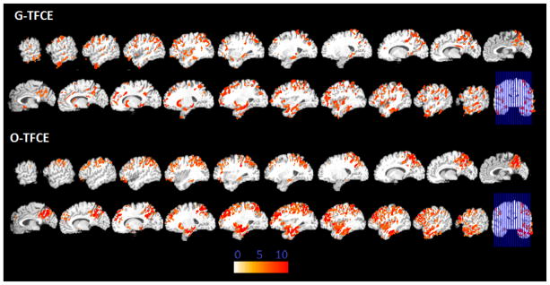
Significant areas of relative decreased gray matter detected by G-TFCE and O-TFCE in the MCI patients. Images are in radiology convention. Multiple voxel comparisons were corrected using the FDR threshold of p<0.05 and a spatial extent threshold of 50 voxels was applied. Color bar indicates −log (p) value. GLM, PS, and WL have no significant findings after FDR correction.

Figure 8.

Significant areas of relative decreased gray matter detected by GLM, PS, WL, G-TFCE, and O-TFCE in the MCI-to-AD converters. Images are in radiology convention. Multiple voxel comparisons were corrected using the FDR threshold of p<0.05 and a spatial extent threshold of 50 voxels was applied. Color bar indicates −log (p) value.

Table 4.

Statistical results of GLM, PS, WL, G-TFCE, and O-TFCER on the group comparison between Schizophrenia patients and normal controls.

Lobe	Region	Side	Number of Voxels					t values
			GLM	PS	WL	G-TFCE	O-TFCE	GLM	PS	WL	G-TFCE	O-TFCE
Frontal Lobe	Orbitofrontal Cortex	R	1538	456	271	1497	1971	6.22	5.94	6.15	5.48	5.79
	Middle Frontal Gyrus	L	203	109	138	1174	1915	6.63	7.6	7.43	6.23	6.51
	Superior Frontal Gyrus	R	385	99	162	1113	1730	6.93	7.73	7.87	6.65	6.84
	Superior Frontal Gyrus	L	86	62	/	761	1594	5.68	5.75	/	6.29	6.77
	Orbitofrontal Cortex	L	1109	227	223	1212	1332	5.11	5.76	6.01	5.82	6.44
	Middle Frontal Gyrus	R	227	94	151	1051	1515	7.07	7.91	8.2	6.62	7.24
	Superior Frontal Gyrus, medial	L	430	112	132	1107	1608	5.15	6.83	6.76	5.68	5.96
	Supplementary Motor Area	L	113	58	60	480	1235	5.18	5.61	5.64	6.45	6.49
	Supplementary motor area	R	182	/	/	461	995	4.17	/	/	5.93	5.88
	Inferior Frontal Gyrus	L	222	61	78	531	635	3.79	5.72	5.81	5.45	5.68
	Precentral Gyrus	L	0	/	/	483	1057	0	/	/	6.26	6.22
	Precentral Gyrus	R	171	51	59	532	914	5.66	4.11	5.21	5.93	6.43
	Superior Frontal Gyrus, medial	R	258	184	206	841	1163	6.25	7.48	7.31	6.02	6.32
	Inferior Frontal Gyrus	R	133	/	/	277	385	4.32	/	/	5.15	5.64
	Paracentral Lobule	L	/	/	/	391	484	0	/	/	5.86	6.43
	Supramarginal Gyrus	R	175	64	67	155	476	3.13	6.76	6.89	6.91	6.91
	Straight Gyrus	L	275	100	109	375	414	5.13	5.38	5.38	4.44	4.49
	Straight Gyrus	R	147	120	138	307	340	4.31	5.33	5.25	4.63	4.78
	Rolandic Operculum	R	294	94	107	623	424	4.74	6.53	6.44	5.04	6.44
	Rolandic Operculum	L	236	80	100	299	185	4.91	6.49	6.36	5.08	5.94
Limbic Lobe	Median Cingulate	R	330	169	250	926	914	6.18	6.47	6.34	5.57	6.25
	Median Cingulate	L	174	95	108	700	815	6.24	5.89	5.92	5.36	5.81
	Hippocampus	R	212	140	142	327	297	4.63	4.96	5.01	5.02	5
	Anterior Cingulate	L	252	54	61	478	450	4.73	5.38	5.32	4.65	5.06
	Parahippocampal Gyrus	R	253	163	159	453	400	4.27	6.03	5.78	4.86	5.15
	Anterior Cingulate	R	114	57	75	228	239	4.97	5.74	5.71	5.07	5.02
	Calcarine Fissure	L	240	66	88	441	278	4.73	6.18	6.05	4.94	5.16
	Hippocampus	L	/	60	61	299	157	0	5.55	5.39	4.43	3.83
	Calcarine Fissure	R	101	73	76	241	159	4.72	5.7	5.7	4.89	5.34
Occipital Lobe	Lingual Gyrus	L	256	118	130	499	415	4.88	7.19	7.3	5.64	6.34
	Inferior Occipital Gyrus	R	165	54	69	250	255	4.55	5.37	4.8	4.51	4.55
	Inferior Occipital Gyrus	L	82	58	56	225	314	3.69	5.27	5.4	5.67	6.04
	Lingual Gyrus	L	141	109	133	430	344	5.06	6.29	6.08	5.04	5.65
	Cuneus	L	98	50	61	297	167	4.24	5.17	6.33	5.24	4.67
	Superior Occipital Gyrus	L	/	/	/	145	121	0	/	/	5.59	4.6
	Middle Occipital Gyrus	L	/	/	/	205	389	0	/	/	5.46	6.79
Parietal Lobe	Precuneus	L	258	74	81	816	967	5.79	6.4	6.04	5.94	6.52
	Postcentral Gyrus	R	373	107	131	719	897	6.2	7.16	6.93	6.67	7.15
	Postcentral Gyrus	L	118	169	250	926	914	6.39	6.47	6.34	5.57	6.25
	Inferior Patietal Gyrus	L	281	123	128	450	591	4.53	7.34	7.11	6.28	6.85
	Inferior Patietal Gyrus	R	324	83	99	297	319	7.48	7.16	7.03	6.3	6.75
	Precuneus	R	129	74	117	801	560	5.64	5.9	5.94	5.4	6.55
	Supramarginal Gyrus	L	/	/	/	161	275	0	/	/	5.3	5.29
	Angular Gyrus	R	/	/	/	63	83	0	/	/	4.2	4.71
Temporal Lobe	Middle Temporal Gyrus	L	1226	345	422	1785	2406	6.57	8.18	7.68	6.56	6.67
	Middle Temporal Gyrus	R	957	435	554	1486	1781	7.7	8.07	7.7	6.71	7.02
	Inferior Temporal Gyrus	L	794	246	287	1030	1282	6.07	7.24	6.87	6	6.12
	Inferior Temporal Gyrus	R	593	242	320	1208	1623	5.94	6.56	6.64	5.55	5.63
	Superior Temporal Gyrus	L	779	210	233	949	961	6.2	7.06	6.97	5.83	6.24
	Fusiform Gyrus	R	450	157	203	862	1052	5.97	6.65	6.29	5.3	5.28
	Superior Temporal Gyrus	R	470	256	288	818	1062	3.64	8.16	7.95	6.32	6.67
	Fusiform Gyrus	L	318	220	249	886	1178	5.82	7.09	6.67	6.25	6.56
	Temporal Pole	R	88	/	/	349	518	3.48	/	/	4.99	5.19
Sub-lobar	Insular Cortex	R	331	185	203	640	396	5.08	6.5	6.23	5.12	5.95
	Insular Cortex	L	353	245	304	756	231	5.7	6.56	6.01	5.35	6.44

Table 5.

Statistical results of GLM, PS, WL, G-TFCE, and O-TFCER on the group comparison between MCI patients and normal controls.

Lobe	Region	Side	Number of Voxels			t values
			G-TFCE	O-TFCE	G-TFCE	O-TFCE
Frontal Lobe	Middle Frontal Gyrus	L	1187	2274	5.33	6.06
	Inferior Frontal Gyrus	L	507	910	4.56	5.13
	Superior Frontal Gyrus	L	870	1303	5.26	5.45
	Precentral Gyrus	L	503	1152	4.72	5.36
	Middle Frontal Gyrus	R	662	962	4.59	6.07
Limbic Lobe	Hippocampus	L	341	456	4.46	4.53
	Parahippocampal Gyrus	L	234	397	4.68	4.16
	Amygdala	L	122	180	3.3	3.41
	Median Cingulate	L	233	275	4.4	4.67
	Posterior Cingulate	L	56	81	4.41	4.33
Parietal Lobe	Precuneus	L	522	1534	3.99	4.47
	Precuneus	R	813	1543	4.78	4.98
	Supeior Patietal Gyrus	L	499	1160	4.42	6.49
	Supeior Patietal Gyrus	R	686	1382	4.21	4.59
	Postcentral Gyrus	L	645	1113	5.56	5.52
	Postcentral Gyrus	R	824	1238	4.81	5.65
	Inferior Patietal Gyrus	L	341	456	4.46	4.53
	Inferior Patietal Gyrus	R	220	508	3.61	3.77
	Angular Gyrus	R	412	510	4.01	4.63
Temporal Lobe	Middle Temporal Gyrus	L	966	1502	4.26	4.63
	Inferior Temporal Gyrus	L	784	1000	4.94	5.26
	Superior Temporal Gyrus	L	575	789	3.85	4.32
	Fusiform Gyrus	L	400	493	4.61	5.01
	Temporal Pole	L	109	295	3.6	3.58
Sub-lobar	Insular Cortex	L	392	561	3.83	4.28

Table 6.

Statistical results of GLM, PS, WL, G-TFCE, and O-TFCER on the group comparison between the MCI-to-AD converters and the Non-converters.

Lobe	Region	Side	Number of Voxels					t values
			GLM	PS	WL G-TFCE		O-TFCE	GLM	PS	WL	G-TFCE	O-TFCE
Frontal Lobe	Orbitofrontal Cortex	L	173	243	248	895	927	3.31	5.29	5.51	4.83	5.54
	Rolandic Operculum	R	236	54	63	600	828	4.26	5.57	5.76	4.57	5.25
	Orbitofrontal Cortex	R	194	112	89	545	730	5.36	5.57	5.67	4.23	4.41
	Precentral Gyrus	R	/	59	75	532	575	/	5.61	5.55	4.57	5.8
	Straight Gyrus	L	136	/	/	282	407	5.43	/	/	3.95	4.05
	Straight Gyrus	R	202	125	155	289	330	3.77	5.25	5.18	4.89	5.38
	Inferior Frontal Gyrus	R	/	183	213	419	494	/	5.81	5.75	4.29	5.63
	Rolandic Operculum	L	84	50	49	195	174	3.46	6.05	5.95	4.78	5.88
	Olfactory Cortex	R	61	79	70	134	170	5.8	5.07	5.19	4.6	4.62
	Olfactory Cortex	L	/	/	/	129	197	/	/	/	4.05	4.12
	Precentral Gyrus	L	82	/	/	449	197	4.11	/	/	5.43	4.12
Limbic Lobe	Parahippocampal Gyrus	R	262	184	198	585	828	4.63	5.53	5.67	4.58	4.48
	Hippocampus	L	512	422	388	638	654	5.56	5.74	5.64	5.12	5.32
	Hippocampus	R	429	279	294	542	659	5.11	5.79	5.79	4.78	4.76
	Parahippocampal Gyrus	L	135	114	106	430	592	4.55	5.1	5.17	4.7	4.21
	Amygdala	R	175	144	143	222	233	3.8	4.19	4.13	4.47	4.59
	Amygdala	L	158	162	161	243	254	4.56	4.86	5.1	4.56	4.49
	Median Cingulate	L	113	56	58	482	137	4.52	5.64	6.07	4.56	6.15
Occipital Lobe	Middle Occipital Gyrus	L	363	82	105	717	694	5.16	6.38	6.24	5.42	6.08
	Inferior Occipital Gyrus	R	97	/	/	315	448	4.47	/	/	4.01	4.97
	Middle Occipital Gyrus	R	89	/	/	542	483	4.99	/	/	4.66	6.22
	Lingual Gyrus	R	/	/	/	461	127	/	/	/	4.8	5.58
	Cuneus	L	/	/	/	279	136	/	/	/	4.32	5.88
	Superior Occipital Gyrus	L	/	50	80	142	153	/	4.72	5.92	4.27	6.52
	Calcarine Fissure	L	246	53	93	852	115	4.44	4.97	4.76	4.21	5.94
	Cuneus	R	58	59	61	225	135	5.63	5.62	5.49	4.38	6.12
	Inferior Occipital Gyrus	L	/	/	/	134	77	/	/	/	4.23	5.39
Parietal Lobe	Postcentral Gyrus	R	378	107	121	802	881	5.52	5.48	5.75	4.89	5.13
	Precuneus	L	188	50	53	864	806	3.45	6.18	6.01	4.79	6.49
	Supramarginal Gyrus	R	160	/	/	376	582	4.09	/	/	4.31	5.43
	Supeior Patietal Gyrus	L	/	/	/	350	357	/	/	/	5.06	6.24
	Precuneus	R	165	82	103	689	498	4.78	6.07	6.03	4.63	6.91
	Angular Gyrus	R	92	57	58	459	246	4.78	5.95	5.88	4.09	6.04
	Angular Gyrus	L	/	/	/	214	124	/	/	/	4.15	6.12
	Inferior Parietal Gyrus	L	/	/	/	302	80	/	/	/	5.16	5.32
Temporal Lobe	Middle Temporal Gyrus	R	541	226	274	1686	2244	5.23	6.47	6.09	4.82	5.44
	Middle Temporal Gyrus	L	984	296	318	2025	2439	5.89	6.26	6.33	5.07	6.07
	Superior Temporal Gyrus	R	1126	316	335	1822	2344	5.04	6.32	5.67	5.05	5.73
	Inferior Temporal Gyrus	R	237	81	106	1243	1755	4.73	4.94	4.92	4.53	5.08
	Inferior Temporal Gyrus	L	243	118	108	954	1606	5.14	5.64	5.26	4.9	5.42
	Temporal Pole	R	153	321	407	1214	1468	4.42	5.76	6.11	4.68	5
	Fusiform Gyrus	R	88	/	/	827	1168	4.26	/	/	4.37	4.94
	Superior Temporal Gyrus	L	709	346	355	972	1061	5.51	7.57	7.5	5.81	6.48
	Fusiform Gyrus	L	144	151	162	854	932	5.22	6.52	6.28	4.94	5.1
	Temporal Pole	L	208	461	460	871	901	4.53	6.85	6.13	5.63	5.66
Sub-lobar	Insular Cortex	R	243	188	191	595	718	5.24	5.12	5.04	4.87	4.85
	Insular Cortex	L	142	147	139	594	593	6.11	6.52	6.34	4.48	4.85
	Putamen	R	/	/	/	144	234	/	/	/	2.85	2.83
	Heschl Gyrus	L	122	72	69	158	156	5.46	5.82	5.71	4.86	5.13
	Heschl Gyrus	R	128	/	/	164	172	3.98	/	/	4.64	4.65
	Putamen	L	/	/	/	214	161	/	/	/	2.95	3

Figure 9.

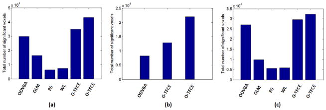
The total number of significant voxels of different methods in three datasets. (a) Group comparison between the schizophrenia patients and the normal controls in Dataset1; (b) Group comparison between the MCI patients and the normal controls in Dataset2; (c) Group comparison between the MCI-to-AD converters and the non-converters in Dataset3.

Figure 10.

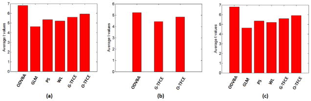
The average t values of anatomical regions of different methods in three datasets. (a) Group comparison between the schizophrenia patients and the normal controls in Dataset1; (b) Group comparison between the MCI patients and the normal controls in Dataset2; (c) Group comparison between the MCI-to-AD converters and the non-converters in Dataset3.

Figure 11.

Results in the local area near the hippocampus. Two representative sections are selected from two analyses: (A) Group comparison between the schizophrenia patients and the normal controls in Dataset1; (B) Group comparison between the MCI-to-AD converters and the non-converters in Dataset3.

Figure 12.

ROC curves of different methods reflecting spatial agreement between detected regions and underlying GM segmentation. The results are obtained from two analyses: (a) Group comparison between the schizophrenia patients and the normal controls in Dataset1; (b) Group comparison between the MCI-to-AD converters and the non-converters in Dataset3.

Table 7.

The accuracy rates and the AUCs of five-folds cross validation on three datasets. The values in the brackets are p values obtained from the paired-differences t test based on the five-fold cross-validated accuracy rates. For Dataset 1 and Dataset 3, GLM is set as baseline. For Dataset 2, ODVBA is set as baseline.

		GLM	PS	WL	ODVBA	G-TFCE	O-TFCE
Dataset1	Accuracy	65.24% (baseline)	66.75% (0.3262)	66.35% (0.3852)	67.06% (0.3725)	69.44% (0.1422)	71.19% (0.0467)
	AUC	0.7013	0.7298	0.7090	0.7212	0.7221	0.7386
Dataset2	Accuracy	/	/	/	66.67% (baseline)	66.67% (0.5000)	70% (0.1870)
	AUC	/	/	/	0.7111	0.7111	0.7867
Dataset3	Accuracy	70% ( baseline)	71% (0.3107)	68% (0.6256)	72% (0.1870)	71% (0.3107)	72% (0.1870)
	AUC	0.6972	0.7496	0.7816	0.7960	0.7752	0.7956

Figure 13.

ROC curves of different methods reflecting classification performances based on detected regions. The results are obtained from three analyses: (a) Group comparison between the schizophrenia patients and the normal controls in Dataset1; (b) Group comparison between the MCI patients and the normal controls in Dataset2; (c) Group comparison between the MCI-to-AD converters and the non-converters in Dataset3.

4 Discussions and Conclusions

Optimally-Discriminative Voxel-Based Analysis (ODVBA), as a new voxel-based morphometry method with a novel spatially adaptive smoothing scheme, is applied to three previously-published studies assessing Schizophrenia, Normal-to-MCI conversion, and MCI-to-AD conversion. The conventional VBM method (Gaussian smoothing plus GLM), two existing spatially adaptive smoothing methods: propagation-separation (PS) and wavelet denosing (WL), and two versions of the Threshold-Free Cluster Enhancement (TFCE) method: G-TFCE and O-TFCE, are also performed for the comparison. ODVBA has been previously validated using extensive simulated atrophy experiments, for which ground truth was available. Therefore, the goal of this paper was to apply ODVBA to three previously-published studies and compare its ability to detect group differences as compared to other methods. There is no ground truth in these three studies; therefore, we focused on measuring 1) the spatial extent of brain regions detected as significantly different between groups, 2) the significance of the group difference, 3) the spatial agreement between detected regions and underlying tissue boundaries, which relates to the blurring effect typically caused by Gaussian smoothing, and 4) classification accuracy based on detected regions.

With ODVBA, we measured widespread regions of significantly lower GM volumes in schizophrenia patients. More than one third of these regions are located in the frontal lobe including the middle frontal gyrus, the orbitofrontal cortex, the superior frontal gyrus, the supplementary motor area, among others. That indicated that the frontal lobe has strong involvement in schizophrenia, and is consistent with the earlier studies (Andreasen et al., 1986, Gur et al., 2000, Davatzikos et al., 2005, Andreasen et al., 2011, Arangoet al., 2012 ). The second largest cluster was located in the temporal lobe, especially the medial area, which is the most frequent region in Honea’s review work (Honea et al., 2005). The main new finding in our study is the significant volume reduction in the bilateral supplementary motor area which however is not reported in our early study (Davatzikos et al., 2005) and recent meta-analysis (Honea et al., 2005, Glahn et al., 2008, Ellison-Wright et al., 2010, Bora et al., 2011). Abnormalities in the supplementary motor area is known (Schroder et al., 1995, Frith et al., 2000, Putzhammer and Klein, 2006) to cause motor disturbances which are common, disabling symptoms in schizophrenic patients. Therefore, the reduction in the size of the bilateral supplementary motor area as demonstrated by ODVBA may imply a link between this region and the debilitating motor disturbances common in schizophrenic patients.

The differences between cognitively normal elderly who remain stable and cognitive normal elderly who convert to MCI are naturally more subtle. The conventional VBM method, using GLM, was unable to find significant differences. However, these regions were detected by ODVBA and had high t values. The regions are in accordance with the early work (Davatzikos et al., 2008), which constructs the spatial map by using the SVM accuracy scores (Lao et al., 2004). However besides the regions in the temporal lobe and the frontal lobe, our new findings are involved with the parietal lobe bilaterally including the precuneus and the superior parietal gyrus which are known to be involved in semantic and visuospatial deficits (Caine and Hodges 2001, Eustache et al, 2004) in mild cognitive impairment and early Alzheimer’s disease. These findings in parietal area agree with some studies with different MCI datasets (Frisoni et al., 2002, Pennanen et al., 2005, Matsuda 2007, Bai et al., 2008, Pihlajamäki et al., 2009, Tondelli et al., 2012).

Our results of ODVBA provided strong evidence that MCI-to-AD converters had already reached levels of widespread and significant brain atrophy at baseline. They confirm our earlier findings (Misra et al., 2009) of gray matter volume reduction in the temporal lobe and the limbic lobe, the orbitofrontal cortex, the precuneous and the insular cortex. Morever, compared with the earlier work, our results also present some new findings, most of which are in agreement with the literature. They include the middle occipital gyrus (Hamalainen et al., 2007), the lingual gyrus (Kinkingnehun et al., 2008), the cuneus (Kinkingnehun et al., 2008), the supramarginal gyrus (Risacher et al., 2010, Schroeter et al., 2009, Bozzali et al., 2006), the angular gyrus (Risacher et al., 2010, Hamalainen et al., 2007, Schroeter et al., 2009, Bozzali et al., 2006), the putamen (Douaud et al., 2011), the heschl’s gyrus, the rolandic operculum, the precentral gyrus, the straight gyrus (Schroeter et al., 2009), the olfactory cortex, and etc. In the literature, these regions are known to be altered in pathology studies of AD. Changes in these regions can be linked with clinical symptoms common in AD patients. For example, changes in the occipital gyrus, lingual gyrus and cuneus can cause visual field defects (Hof and Morrison, 1990, Armstrong, 1996); atrophies in the supramarginal and angular gyrus can be reflected by language impairments (Harasty et al, 1999, Ullman et al, 1997); and as a part of the auditory system, the loss of heschl’s gyrus may lead to certain auditory deficits (Goll et al, 2011).

For comparison, ODVBA demonstrated highest significance in group differences within the identified voxels. In terms of spatial agreement of boundary, ODVBA and the two cluster enhancing methods: O-TFCE and G-TFCE performed the best, while GLM performed the worst, since it tends to blur the true structure of the group difference and do not necessarily conform to the shape of the underlying pathology. With regard to the spatial extent of the detected significant area, ODVBA produced the highest sensitivity of the voxel-based methods. G-TFCE and O-TFCE, as the cluster enhancing methods, demonstrated enhanced statistical power, with O-TFCE outperforming G-TFCE, thereby indicating the synergistic value between ODVBA and TFCE. In addition, in experiments based on classification, ODVBA demonstrated a slight advantage over the other voxel-based methods, and O-TFCE displayed an enhanced performance. In conclusion, ODVBA showed overall higher performance, at least for the criteria tested. In terms of agreement of anatomical boundary, spatial extent of detected area, and classification, it performed competitively with both cluster enhancing methods. It is worth noting that for all tested criteria, O-TFCE performed better than the original G-TFCE, thereby indicating the synergistic value between ODVBA and TFCE.

Two typical spatially adaptive smoothing methods: propagation-separation (PS) and wavelet denosing (WL) have been performed for comparison purpose. The experimental results demonstrated the stability of the two methods with varying smoothing kernel sizes, and excellent specificity in terms of agreement of tissue boundary especially shown in Figure 12(a). However, it’s also shown that PS and WL have limited sensitivity to detect the group difference. The reason is that the two methods smooth each single subject separately and do not enhance the discriminative information derived from population. Recently, there is some related work having great potential to tackle this problem. For example, MARM as well as its variant (Li et al 2011, Li et al 2012), has been proposed to extend the original PS method to the case of multiple subjects by incorporating the voxel-wise general statistical modeling for regression analysis. We will investigate their possible applications on two-group comparison analysis in our future work.

References

- Andreasen N, Nasrallah HA, Dunn V, Olson SC, Grove WM, Ehrhardt JC, Coffman JA, Crossett JH. Structural abnormalities in the frontal system in schizophrenia. A magnetic resonance imaging study. Arch Gen Psychiatry. 1986;43:136–144. doi: 10.1001/archpsyc.1986.01800020042006. [DOI] [PubMed] [Google Scholar]
- Andreasen NC, Nopoulos P, Magnotta V, Pierson R, Ziebell S, Ho BC. Progressive brain change in schizophrenia: a Prospective longitudinal study of first-episode schizophrenia. Biol Psychiatry. 2011;70:672–679. doi: 10.1016/j.biopsych.2011.05.017. [DOI] [PMC free article] [PubMed] [Google Scholar]
- Arango C, Rapado-Castro M, Reig S, Castro-Fornieles J, González-Pinto A, Otero S, Baeza I, Moreno C, Graell M, Janssen J, Parellada M, Moreno D, Bargalló N, Desco M. Progressive brain changes in children and adolescents with firstepisode psychosis. Arch Gen Psychiatry. 2012;69 (1):16–26. doi: 10.1001/archgenpsychiatry.2011.150. [DOI] [PubMed] [Google Scholar]
- Armstrong RA. Visual field defects in Alzheimer’s disease patients may reflect differential pathology in the primary visual cortex. Optometry and vision science. 1996;73(11):677–682. doi: 10.1097/00006324-199611000-00001. [DOI] [PubMed] [Google Scholar]
- Ashburner J, Friston KJ. Voxel-based morphometry—the methods. NeuroImage. 2000;11:805–821. doi: 10.1006/nimg.2000.0582. [DOI] [PubMed] [Google Scholar]
- Ashburner J, Csernansky JG, Davatzikos C, Fox NC, Frisoni GB, Thompson PM. Computer-assisted imaging to assess brain structure in healthy and diseased brains. Lancet Neurol. 2003;2 (2):79–88. doi: 10.1016/s1474-4422(03)00304-1. [DOI] [PubMed] [Google Scholar]
- Bai F, Zhang Z, Yu H, Shi Y, Yuan Y, Zhu W, Zhang X, Qian Y. Default-mode network activity distinguishes amnestic type mild cognitive impairment from healthy aging: a combined structural and resting-state functional MRI study. Neurosci Lett. 2008;438:111–115. doi: 10.1016/j.neulet.2008.04.021. [DOI] [PubMed] [Google Scholar]
- Bora E, Fornito A, Radua J, Walterfang M, Seal M, Wood SJ, Yucel M, Velakoulis D, Pantelis C. Neuroanatomical abnormalities in schizophrenia: a multimodal voxelwise meta-analysis and meta-regression analysis. Schizophr Res. 2011;127:46–57. doi: 10.1016/j.schres.2010.12.020. [DOI] [PubMed] [Google Scholar]
- Bozzali M, Filippi M, Magnani G, Cercignani M, Franceschi M, Schiatti E, Castiglioni S, Mossini R, Falautano M, Scotti G, Comi G, Falini A. The contribution of voxel-based morphometry in staging patients with mild cognitive impairment. Neurology. 2006;67:453–460. doi: 10.1212/01.wnl.0000228243.56665.c2. [DOI] [PubMed] [Google Scholar]
- Caine D, Hodges JR. Heterogeneity of semantic and visuospatial deficits in early Alzheimer’s disease. Neuropsychology. 2001;15(2):155–164. [PubMed] [Google Scholar]
- Chang CC, Lin CJ. LIBSVM: a library for support vector machines. ACM Transactions on Intelligent Systems and Technology. 2011;2(3):27. [Google Scholar]
- Davatzikos C, Fan Y, Wu X, Shen D, Resnick SM. Detection of prodromal Alzheimer’s disease via pattern classification of magnetic resonance imaging. Neurobiol Aging. 2008;29:514–523. doi: 10.1016/j.neurobiolaging.2006.11.010. [DOI] [PMC free article] [PubMed] [Google Scholar]
- Davatzikos C, Shen D, Gur RC, Wu X, Liu D, Fan Y, Hughett P, Turetsky BI, Gur RE. Whole-brain morphometric study of schizophrenia revealing a spatially complex set of focal abnormalities. Arch Gen Psychiatry. 2005;62:1218–1227. doi: 10.1001/archpsyc.62.11.1218. [DOI] [PubMed] [Google Scholar]
- Davatzikos C, Genc A, Xu D, Resnick SM. Voxel-based morphometry using the RAVENS maps: methods and validation using simulated longitudinal atrophy. NeuroImage. 2001a;14:1361–1369. doi: 10.1006/nimg.2001.0937. [DOI] [PubMed] [Google Scholar]
- Davatzikos C, Li HH, Herskovits E, Resnick SM. Accuracy and sensitivity of detection of activation foci in the brain via statistical parametric mapping: a study using a PET simulator. NeuroImage. 2001b;13:176–184. doi: 10.1006/nimg.2000.0655. [DOI] [PubMed] [Google Scholar]
- Dietterich TG. Approximate statistical tests for comparing supervised classification learning classifiers. Neural Computation. 1998;10:1895–1923. doi: 10.1162/089976698300017197. [DOI] [PubMed] [Google Scholar]
- Douaud G, Menke1 R, Gass A, Monsch A, Sollberger M, Rao A, Whitcher B, Matthews P, Smith S. Structural differences can be found between MCI converters and non-converters more than 2 years prior to conversion to AD, Proc. ISMRM. 2011;19:687. [Google Scholar]
- Ellison-Wright I, Bullmore E. Anatomy of bipolar disorder and schizophrenia: a meta-analysis. Schizophr Res. 2010;117:1–12. doi: 10.1016/j.schres.2009.12.022. [DOI] [PubMed] [Google Scholar]
- Eustache F, Piolino P, Giffard B, Viader F, Sayette VDL, Baron JC, Desgranges B. ‘In the course of time’: a PET study of the cerebral substrates of autobiographical amnesia in Alzheimer’s disease. Brain. 2004;127(7):1549–1560. doi: 10.1093/brain/awh166. [DOI] [PubMed] [Google Scholar]
- Frisoni GB, Testa C, Zorzan A, Sabattoli F, Beltramello A, Soininen H, Laakso MP. Detection of grey matter loss in mild Alzheimer’s disease with voxel based morphometry. J Neurol Neurosurg Psychiatry. 2002;73:657–664. doi: 10.1136/jnnp.73.6.657. [DOI] [PMC free article] [PubMed] [Google Scholar]
- Friston K, Holmes A, Worsley K, Poline J, Frith CD, Frackowiak RSJ. Statistical parametric maps in functional imaging: a general linear approach. Hum Brain Mapp. 1994;2:189–210. [Google Scholar]
- Frith CD, Blakemore SJ, Wolpert DM. Explaining the symptoms of schizophrenia: abnormalities in the awareness of action. Brain Research Reviews. 2000;31(2–3):357–363. doi: 10.1016/s0165-0173(99)00052-1. [DOI] [PubMed] [Google Scholar]
- Genovese CR, Lazar NA, Nichols T. Thresholding of statistical maps in functional neuroimaging using the false discovery rate. Neuroimage. 2002;15(4):870–878. doi: 10.1006/nimg.2001.1037. [DOI] [PubMed] [Google Scholar]
- Gerig G, Kubler O, Kikinis R, Jolesz F. Nonlinear anisotropic fionlinea of MRI data. IEEE Trans Med Imaging. 1992;2:221–232. doi: 10.1109/42.141646. [DOI] [PubMed] [Google Scholar]
- Glahn DC, Laird AR, Ellison-Wright I, Thelen SM, Robinson JL, Lancaster JL, Bullmore E, Fox PT. Meta-analysis of gray matter anomalies in schizophrenia: application of anatomic likelihood estimation and network analysis. Biol Psychiatry. 2008;64 (9):774–781. doi: 10.1016/j.biopsych.2008.03.031. [DOI] [PMC free article] [PubMed] [Google Scholar]
- Goldszal AF, Davatzikos C, Pham DL, Yan MX, Bryan RN, Resnick SM. An image-processing system for qualitative and quantitative volumetric analysis of brain images. J Comput Assist Tomogr. 1998;22 (5):827–837. doi: 10.1097/00004728-199809000-00030. [DOI] [PubMed] [Google Scholar]
- Goll JC, Kim LG, Hailstone JC, Lehmann M, Buckley A, Crutch SJ, Warren JD. Auditory object cognition in dementia. Neuropsychologia. 2011;49(9):2755–2765. doi: 10.1016/j.neuropsychologia.2011.06.004. [DOI] [PMC free article] [PubMed] [Google Scholar]
- Good CD, Johnsrude IS, Ashburner J, Henson RN, Friston KJ, Frackowiak RS. A voxel-based morphometric study of ageing in 465 normal adult human brains. NeuroImage. 2001;14:21–36. doi: 10.1006/nimg.2001.0786. [DOI] [PubMed] [Google Scholar]
- Gur RE, Cowell PE, et al. Reduced dorsal and orbital prefrontal gray matter volumes in schizophrenia. Arch Gen Psychiatry. 2000;57 (8):761–768. doi: 10.1001/archpsyc.57.8.761. [DOI] [PubMed] [Google Scholar]
- Hamalainen A, Tervo S, Grau-Olivares M, Niskanen E, Pennanen C, Huuskonen J, Kivipelto M, Hanninen T, Tapiola M, Vanhanen M, Hallikainen M, Helkala EL, Nissinen A, Vanninen R, Soininen H. Voxel-based morphometry to detect brain atrophy in progressive mild cognitive impairment. NeuroImage. 2007;37:1122–1131. doi: 10.1016/j.neuroimage.2007.06.016. [DOI] [PubMed] [Google Scholar]
- Harasty JA, Halliday GM, Kril JJ. Specific temporoparietal gyral atrophy reflects the pattern of language dissolution in Alzheimer’s disease. Brain. 1999;122(4):675–686. doi: 10.1093/brain/122.4.675. [DOI] [PubMed] [Google Scholar]
- Hayasaka S, Phan KL, Liberzon I, Worsley KJ, Nichols TE. Nonstationary cluster-size inference with random field and permutation methods. Neuroimage. 2004;22(2):676–687. doi: 10.1016/j.neuroimage.2004.01.041. [DOI] [PubMed] [Google Scholar]
- Hayasaka S, Nichols TE. Validating cluster size inference: random field and permutation methods. Neuroimage. 2003;20(4):2343–2356. doi: 10.1016/j.neuroimage.2003.08.003. [DOI] [PubMed] [Google Scholar]
- Hof PR, Morrison JH. Quantitative analysis of a vulnerable subset of pyramidal neurons in Alzheimer’s disease: II. Primary and secondary visual cortex. The Journal of comparative neurology. 1990;301(1):55–64. doi: 10.1002/cne.903010106. [DOI] [PubMed] [Google Scholar]
- Holmes AP, Blair RC, Watson JD, Ford I. Nonparametric analysis of statistic images from functional mapping experiments. J Cereb Blood Flow Metab. 1996;16:7–22. doi: 10.1097/00004647-199601000-00002. [DOI] [PubMed] [Google Scholar]
- Honea R, Crow TJ, Passingham D, Mackay CE. Regional deficits in brain volume in schizophrenia: a meta-analysis of voxel-based morphometry studies. Am J Psychiatry. 2005;162 (12):2233–2245. doi: 10.1176/appi.ajp.162.12.2233. [DOI] [PubMed] [Google Scholar]
- Jolliffe I. Principal component analysis. John Wiley & Sons, Ltd; 2005. [Google Scholar]
- Jones DK, Symms MR, Cercignani M, Howard RJ. The effect of filter size on VBM analysesof DT -MRI data. NeuroImage. 2005;26:546–554. doi: 10.1016/j.neuroimage.2005.02.013. [DOI] [PubMed] [Google Scholar]
- Kinkingnehun S, Sarazin M, Lehericy S, Guichart-Gomez E, Hergueta T, Dubois B. VBM anticipates the rate of progression of Alzheimer disease: a 3-year longitudinal study. Neurology. 2008;70:2201–2211. doi: 10.1212/01.wnl.0000303960.01039.43. [DOI] [PubMed] [Google Scholar]
- Lao Z, Shen D, Xue Z, Karacali B, Resnick SM, Davatzikos C. Morphological classification of brains via high-dimensional shape transformations and machine learning methods. NeuroImage. 2004;21:46–57. doi: 10.1016/j.neuroimage.2003.09.027. [DOI] [PubMed] [Google Scholar]
- Li Y, Zhu H, Shen D, Lin W, Gilmore JH, Ibrahim JG. Multiscale adaptive regression models for neuroimaging data. Journal of the Royal Statistical Society: Series B. 2011;73:559–578. doi: 10.1111/j.1467-9868.2010.00767.x. [DOI] [PMC free article] [PubMed] [Google Scholar]
- Li Y, Gilmore JH, Wang J, Styner M, Lin W, Zhu H. TwinMARM: Two-stage Multiscale Adaptive Regression Methods for twin neuroimaging data. IEEE Trans Med Imaging. 2012;31:1100–1112. doi: 10.1109/TMI.2012.2185830. [DOI] [PMC free article] [PubMed] [Google Scholar]
- Maldjian JA, Laurienti PJ, Burdette JB. Precentral gyrus discrepancy in electronic versions of the Talairach atlas. NeuroImage. 2004;21:450–455. doi: 10.1016/j.neuroimage.2003.09.032. [DOI] [PubMed] [Google Scholar]
- Maldjian JA, Laurienti PJ, Burdette JB, Kraft RA. An automated method for neuroanatomic and cytoarchitectonic atlas-based interrogation of fMRI data sets. NeuroImage. 2003;19:1233–1239. doi: 10.1016/s1053-8119(03)00169-1. [DOI] [PubMed] [Google Scholar]
- Matsuda H. The role of neuroimaging in mild cognitive impairment. Neuropathology. 2007;27:570–577. doi: 10.1111/j.1440-1789.2007.00794.x. [DOI] [PubMed] [Google Scholar]
- Misra C, Fan Y, Davatzikos C. Baseline and longitudinal patterns of brain atrophy in MCI patients, and their use in prediction of short-term conversion to AD: results from ADNI. NeuroImage. 2009;44(4):1415–1422. doi: 10.1016/j.neuroimage.2008.10.031. [DOI] [PMC free article] [PubMed] [Google Scholar]
- Nichols TE, Hayasaka S. Controlling the familywise error rate in functional neuroimaging: a comparative review. Stat Methods Med Res. 2003;12 (5):419–446. doi: 10.1191/0962280203sm341ra. [DOI] [PubMed] [Google Scholar]
- Nichols TE, Holmes AP. Nonparametric permutation tests for functional neuroimaging: a primer with examples. Hum Brain Mapp. 2002;15:1–25. doi: 10.1002/hbm.1058. [DOI] [PMC free article] [PubMed] [Google Scholar]
- Pennanen C, Testa C, Laakso MP, Hallikainen M, Helkala EL, Hanninen T, Kivipelto M, Kononen M, Nissinen A, Tervo S, Vanhanen M, Vanninen R, Frisoni GB, Soininen H. A voxel based morphometry study on mild cognitive impairment. J Neurol Neurosurg Psychiatry. 2005;76:11–14. doi: 10.1136/jnnp.2004.035600. [DOI] [PMC free article] [PubMed] [Google Scholar]
- Perona P, Malik J. Scale-space and edge detection using anisotropic diffusion. IEEE Trans Pattern Anal Mach Intell. 1990;12 (7):629–63. [Google Scholar]
- Pihlajamäki M, Jauhiainen AM, Soininen H. Structural and functional MRI in mild cognitive impairment, Curr. Alzheimer Res. 2009;6:179–185. doi: 10.2174/156720509787602898. [DOI] [PubMed] [Google Scholar]
- Pizurica A, Philips W, Lemahieu I, Acheroy M. A versatile wavelet domain noise ltration technique for medical imaging. IEEE Trans Med Imaging. 2003;22:323–331. doi: 10.1109/TMI.2003.809588. [DOI] [PubMed] [Google Scholar]
- Polzehl J, Spokoiny V. Adaptive weights smoothing with applications to image restoration. J R Statist Soc B. 2000;62:335–354. [Google Scholar]
- Polzehl J, Spokoiny V. Local likelihood modeling by adaptive weights smoothing. Probab Theor Relat Fields. 2006;135:335–362. [Google Scholar]
- Putzhammer A, Klein HE. Quantitative analysis of motor disturbances in schizophrenic patients. Dialogues in clinical neuroscience. 2006;8(1):123–130. doi: 10.31887/DCNS.2006.8.1/aputzhammer. [DOI] [PMC free article] [PubMed] [Google Scholar]
- Risacher SL, Shen L, West JD, Kim S, McDonald BC, Beckett La, Harvey DJ, Jack CR, Weiner MW, Saykin AJ. Longitudinal MRI atrophy biomarkers: relationship to conversion in the ADNI cohort. Neurobiol Aging. 2010;31:1401–1418. doi: 10.1016/j.neurobiolaging.2010.04.029. [DOI] [PMC free article] [PubMed] [Google Scholar]
- Salimi-Khorshidi G, Smith SM, Nichols TE. Adjusting the neuroimaging statistical inferences for nonstationarity. Med Image Comput Comput Assist Interv. 2009;12(1):992–999. doi: 10.1007/978-3-642-04268-3_122. [DOI] [PubMed] [Google Scholar]
- Schroeter ML, Stein T, Maslowski N, Neumann J. Neural correlates of Alzheimer’s disease and mild cognitive impairment: A systematic and quantitative meta-analysis involving 1351 patients. NeuroImage. 2009;47:1196–1206. doi: 10.1016/j.neuroimage.2009.05.037. [DOI] [PMC free article] [PubMed] [Google Scholar]
- Schroder J, Wenz F, Schad LR, Baudendistel K, Knopp MV. Sensorimotor cortex and supplementary motor area changes in schizophrenia. A study with functional magnetic resonance imaging. The British Journal of Psychiatry. 1995;167(2):197–201. doi: 10.1192/bjp.167.2.197. [DOI] [PubMed] [Google Scholar]
- Shen D, Davatzikos C. HAMMER: hierarchical attribute matching mechanism for elastic registration. IEEE Trans Med Imag. 2002;21:1421–1439. doi: 10.1109/TMI.2002.803111. [DOI] [PubMed] [Google Scholar]
- Smith SM, Nichols TE. Threshold-free cluster enhancement: Addressing problems of smoothing, threshold dependence and localisation in cluster inference. NeuroImage. 2009;44(1):83–98. doi: 10.1016/j.neuroimage.2008.03.061. [DOI] [PubMed] [Google Scholar]
- Tabelow K, Polzehl J, Voss HU, Spokoiny V. Analyzing fMRI experiments with structural adaptive smoothing procedures. NeuroImage. 2006;33:55–62. doi: 10.1016/j.neuroimage.2006.06.029. [DOI] [PubMed] [Google Scholar]
- Tondelli M, Wilcock GK, Nichelli PD, Jager CA, Jenkinson M, Zamboni G. Structural MRI changes detectable up to ten years before clinical Alzheimer’s disease, Neurobio. Aging. 2012;33:825.e25–825.e36. doi: 10.1016/j.neurobiolaging.2011.05.018. [DOI] [PubMed] [Google Scholar]
- Tzourio-Mazoyer N, Landeau B, Papathanassiou D, Crivello F, Etard O, Delcroix N, Mazoyer B, Joliot M. Automated anatomical labeling of activations in GLM using a macroscopic anatomical arcellation of the MNI MRI single-subject brain. NeuroImage. 2002;15:273–289. doi: 10.1006/nimg.2001.0978. [DOI] [PubMed] [Google Scholar]
- Ullman MT, Corkin S, Coppola M, Hickok G, Growdon JH, Koroshetz WJ, Pinker S. A neural dissociation within language: Evidence that the mental dictionary is part of declarative memory, and that grammatical rules are processed by the procedural system. Journal of cognitive neuroscience. 1997;9(2):266–276. doi: 10.1162/jocn.1997.9.2.266. [DOI] [PubMed] [Google Scholar]
- Zhang T, Davatzikos C. ODVBA: Optimally-Discriminative Voxel Based Analysis. IEEE Trans Med Imaging. 2011;30 (8):1441–1454. doi: 10.1109/TMI.2011.2114362. [DOI] [PMC free article] [PubMed] [Google Scholar]
- Zhang Y, Zou P, Mulhern RK, Butler RW, Laningham FH, Ogg RJ. Brain structural abnormalities in survivors of pediatric posterior fossa brain tumors: A voxel-based morphometry study using free-form deformation. NeuroImage. 2008;42(1):218–229. doi: 10.1016/j.neuroimage.2008.04.181. [DOI] [PMC free article] [PubMed] [Google Scholar]