Large-Volume Reconstruction of Brain Tissue from High-Resolution Serial Section Images Acquired by SEM-Based Scanning Transmission Electron Microscopy

Abstract

With recent improvements in instrumentation and computational tools, serial section electron microscopy has become increasingly straightforward. A new method for imaging ultrathin serial sections is developed based on a field emission scanning electron microscope fitted with a transmitted electron detector. This method is capable of automatically acquiring high-resolution serial images with a large field size and very little optical and physical distortions. In this chapter, we describe the procedures leading to the generation and analyses of a large-volume stack of high-resolution images (64 μm × 64 μm × 10 μm, or larger, at 2 nm pixel size), including how to obtain large-area serial sections of uniform thickness from well-preserved brain tissue that is rapidly perfusion-fixed with mixed aldehydes, processed with a microwave-enhanced method, and embedded into epoxy resin.

1. Introduction

Ever since the presence of synaptic junctions was demonstrated by transmission electron microscopy (TEM) in the 1950s (1, 2), serial thin sections of <100 nm thickness were used to visualize them in the three-dimensional context of the surrounding dendrites, axons, and astroglial process, namely, the “neuropil” (3–6). Recently, serial section EM has gained renewed interest in neuroscience as a high-resolution 3D tool (7) . It has been used for 3D reconstruction of functionally identified local circuitry (8, 9), as well as for attempts to map all synaptic connections in the brain (termed “connectomics”) (10–12). Our laboratory and others use serial section EM to understand how the structure of synapses is modified by experience (or in models of learning and memory), which can ultimately alter the connection profile for a neuron (13–15). In this case, a pixel size of ≤2 nm is required for reliable identification and analyses of subcellular structures (e.g., polyribosomes, microtubules, and smooth endoplasmic reticulum) that may play crucial roles in structural plasticity of synapses.

In order to implement the appropriate serial section EM system to address a particular set of scientific questions, one must consider the features that ultimately determine the system's limitations. These include (but are not limited to): platform (e.g., scanning vs. transmission EM), imaging mode (e.g., detection of transmitted vs. back-scattered electrons), serial sectioning method (e.g., diamond knife vs. focused ion beam), specimen presentation (e.g., block face vs. ultrathin sections), and imaging field size. Two serial section EM systems are based on scanning electron microscopy (SEM) with the detection of back-scattered electrons from the block face that is serially removed either by focused ion beam (FIB-SEM) (16–19) or diamond knife inside the SEM chamber (SBFSEM) (20). These approaches can generate thinner sections (~25 nm for SBFSEM and ~5 nm for FIB-SEM) than the sections obtained for traditional serial EM (~45 nm). Thus, the voxels obtained through FIB-SEM imaging can be more isotropic (several nanometers per side). The FIB-SEM is limited by the size of the field that can be milled and imaged, usually less than 100 μm × 100 μm. The destructive nature of SBFSEM and FIB-SEM precludes post-embedding immunolabeling, reexamination of areas of interest at a higher magnification, or use of EM tomography, which can generate virtual sections of less than 3 nm thickness. In other serial section EM approaches, the images are acquired from ultrathin sections. They can be collected automatically on electron-opaque plastic tapes (automatic tape-collecting lathe ultramicrotome, or ATLUM) (21) or manually on glass microscope slides (array tomography) (22) that can be archived for repeated SEM and light microscopy imaging. Array tomography provides a relatively straightforward platform for immunolabeling and correlative fluorescence and electron microscopy. Serial sections collected on traditional TEM grids can be imaged with a TEM custom-fitted with an array of CCD cameras (TEMCA), which rapidly acquires images with larger field size (8). However, TEMCA is cumbersome and expensive, and the resulting images can still suffer from the specimen drifting, optical distortion, and beam damage that are inherent in TEM imaging.

We have recently developed a new method for imaging serial sections using scanning transmission electron microscopy (STEM) based on a field emission (FE) SEM fitted with a multi-mode transmitted electron detector (23). This system allows for semiautomated acquisition of large-field images (single field size of 64 μm × 64 μm square, or more with mosaic) at a high resolution (1 or 2 nm pixel size) from multiple grids spanning an entire series of ≥200 serial sections loaded on a single specimen holder (with multiple holders, the total section number is only limited by how many can be sectioned). Images taken on this system have less optical distortion and specimen drift, and the resolution is comparable to those taken on a conventional TEM with a bottom-mount CCD camera (pixel dimension = 4,080 × 4,080) at a magnification of about 5,000×. Archived serial sections on conventional TEM grids can be imaged on this SEM system without modification. In addition, less operator involvement is required, and the instrument can be obtained for about half the cost of a conventional TEM with a large-format CCD camera. Recent improvements in computational tools are also making it easier to handle large-field serial images for alignment and analysis, as well as to generate realistic three-dimensional reconstructions of segmented objects (24–32).

In order to take advantage of these advanced tools for studying structural plasticity, however, one must start with well-preserved brain tissue, which can be achieved by rapid perfusion-fixation with mixed aldehydes while the animal is under artificial ventilation to minimize hypoxic damages (33). Once well-fixed tissue undergoes microwave-enhanced processing and is embedded into epoxy resin (34), serial thin sections of uniform thickness (~45 nm) must be obtained from a precisely targeted brain region of interest while minimizing flaws, such as folds, knife marks, and debris from stain or dust (35). The following describes our routine methods to generate series of high-quality EM images from neuropil in the hippocampal dentate gyrus of perfusion-fixed brain tissue embedded in epoxy resin. The resulting image series is then used for quantitative analyses and three-dimensional reconstruction of neuronal and glial structures.

2. Materials

General reagents, equipment, and supplies include: purified water (double-distilled or 18 MΩ), 1 N aqueous NaOH, 1 N aqueous HCl, balance, forceps, glassware (e.g., beakers, cylinders, flasks, petri dish, and vials), hot plate stirrer, osmometer, small paint brush, pH meter, sonicator, cyanoacrylate glue (e.g., Super Glue®), desiccant, filter paper, glass microscope slides and cover glass (#1 thickness), Kimwipes® , Parafilm M®, pipettes, razor blades, syringes, syringe filters (pore size = 0.22 μm).

2.1. Perfusion-Fixation

1. Animals: Adult rats (typically 4–6 months old; see Note 1). They can be naïve, or ones that underwent in vivo experiments such as electrophysiological recordings or behavioral learning.

2. Anesthetics (halothane or isoflurane; see Note 2), vaporizer (Midmark), and a large desiccator jar.

3. Surgical tools such as scalpels, scissors, suture, forceps, hemostats, bone rongeurs, and spatulas.

4. Perfusion apparatus (Fig. 1): dissection tray, Styrofoam board, pins, O₂/CO₂ (95%/5%) tank and regulator, small animal ventilator, nose cone, sphygmomanometer (with the cuff cut off), water bath, 2-L glass bottles, hypodermic needles. These components are assembled with an assortment of stoppers, tubing, connectors, clamps, and valves (see Note 3).

5. Krebs-Ringer Carbicarb buffer (KRC): 2.0 mM CaCl₂, 11.0 mM d-glucose, 4.7 mM KCl, 4.0 mM MgSO₄, 118 mM NaCl, 12.5 mM Na₂CO₃, 12.5 mM NaHCO₃, pH = 7.35–7.4, osmolality = 300–330 mmol/kg (see Note 4).

6. Fixative: 2.0% formaldehyde, 2.5% glutaraldehyde, 2 mM CaCl₂, 4 mM MgSO₄, 100 mM sodium cacodylate, pH = 7.35 (aldehydes and sodium cacodylate are obtained from Ladd Research; see Note 5).

7. Vacuum filter system (pore size = 0.22 μm) to filter KRC and fixative.

Fig. 1.

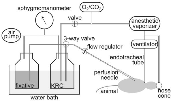
A simplified diagram of the perfusion apparatus as described in Subheadings 2.1 and 3.1.

2.2. Tissue Processing

1. Vibrating blade microtome.

2. 24-well plates.

3. 0.1 M phosphate buffer, pH 7.4.

4. Dissecting microscope.

5. Small dissecting knife, ~4 mm cutting edge (Fine Science Tools).

6. 0.1 M sodium cacodylate buffer, pH 7.4.

7. Agarose: 7% in purified water.

8. Laboratory microwave oven with vacuum chamber and cooling stage (Ted Pella): prior to tissue processing, the magnetron needs to be warmed up by running it for 2 min at 175 W.

9. Tissue processing basket (Ted Pella).

10. Reduced osmium: 1% osmium tetroxide (see Note 6) and 1.5% potassium ferrocyanide [K₄Fe(CN)₆ 3H₂O] in sodium cacodylate buffer.

11. 1% Osmium tetroxide in sodium cacodylate buffer (see Note 6).

12. Uranyl acetate (ACS reagent grade).

13. Ethanol (see Note 7).

14. Propylene oxide.

15. LX-112 epoxy resin embedding kit (Ladd Research).

16. Rotator.

17. Chien embedding mold (Electron Microscopy Sciences, Polysciences, or Ted Pella).

18. Laboratory oven.

2.3. Ultramicrotomy and Post-section Staining

1. SynapTek™ beryllium-copper slot grids, slot size = 1 mm × 2 mm or 0.5 mm × 2 mm (Ted Pella or Electron Microscopy Sciences).

2. Pioloform® F (Ted Pella): 0.7% solution in high-purity chloroform.

3. Supplies for casting Pioloform films, including a film casting device (Electron Microscopy Sciences), Ross optical lens tissue paper, 70% ethanol, Alconox® (saturated aqueous solution filtered and diluted to ~20%), and a large glass container (to contain water on which Pioloform films are floated).

4. Ultramicrotome (Leica Microsystems), placed in a Plexiglas enclosure on an air table in a dedicated room (Fig. 2g).

5. Diamond trim knife (DiATOME cryotrim 20).

6. Diamond thin-sectioning knife (DiATOME ultra 35).

7. Supplies for manipulating and picking up serial sections such as eyelash, forceps, and grid box.

8. Grid staining dish (with lid): 55 mm glass Petri dish filled with melted dental wax. Indentations are made on the wax surface with a razor blade so that grids can be inserted vertically.

9. Uranyl acetate: Saturated aqueous solution. Add 6.25 g of uranyl acetate to 100 ml of purified water and sonicate for up to 1 h. Store at 4°C.

10. Reynolds' lead citrate stain (36): In purified water boiled to expel CO₂, completely dissolve lead nitrate (Ladd Research) for the final concentration of 2.66%, then sodium citrate (3.52% final). The solution will turn milky white. After letting stand for 30 min with occasional mixing, add fresh aqueous sodium hydroxide (0.16 N final) (see Note 8). To avoid exposure to air, store in 10 ml syringes with syringe filer and hypodermic needle stuck on a rubber stopper at 4°C.

11. Sodium hydroxide: some pellets and 0.02 N aqueous solution.

Fig. 2.

(a) Dorsal view of a perfusion-fixed adult rat brain. Dotted black line indicates an approximate location from which the slice shown in b and b′ was taken on a vibrating blade microtome. (b) A parasagittal slice of the hippocampus. Area CA1 and the dentate gyrus (DG) are indicated. (b′) The same slice as in b, with a superimposed image of the dentate tissue embedded in the epoxy block shown in c. (c) An epoxy block containing the dentate tissue dissected from the slice shown in b and b′. The Chien embedding mold was used so that the tissue can be cut from two faces of the block (C with dotted line = “cross-section face”; L with solid line = “longitudinal face”). (c′) A diagram indicating the orientation of the tissue in the block shown in c . The “cross-section face” (C) is parallel to the granule cell layer (gray spheres), and dendrites (gray curved lines in the molecular layer) of these cells are cut in cross section in this plane. The “longitudinal face” (L) is perpendicular to the cell layer and the cross-section face, and therefore the dendrites are cut longitudinally in this plane. In this example, serial sections are cut from the cross-section face at 125 μm from the top of the granule cell layer (i.e., middle molecular layer). (d) An electron micrograph of a test-thin section cut from the longitudinal face of the block shown in c. This image is used to determine how much of the tissue must be trimmed to reach the target location on the cross-section face (i.e., 517 − 125 μm = 392 μm to trim). The rectangle with dotted line indicates the area imaged in E after trimming. “Hash” corresponds to the location of capillary seen in E. Note that flaws in the thin section or Pioloform film (e.g., folds) cannot be avoided in sections of this size (also see e), but they are minimized in serial sections cut from a much smaller block face (see h). (e) An electron micrograph of another test-thin section, taken after trimming to the target location. The target (125 μm) will be well within a series of 200 serial sections (spanning about 9 μm), so the final block face is trimmed at this point. (f) A diagram showing the final block face (gray trapezoid area) trimmed on the cross-section face of the block. The asterisk (also in f′ and h) indicates the “reference corner”: the edge extending into tissue from this corner is perpendicular to the block face, and therefore remains constant throughout the series. (f′): The top-down view of the longitudinal face of the block in f, depicting the method for trimming the top and bottom edges of the block face. After the bottom edge is trimmed with a 20° slope, the knife is turned 20° to the right, so that the top edge is trimmed to become perpendicular to the block face. (g) In a dedicated room, the ultramicrotome (u) is placed in a Plexiglas enclosure (e) on an air table (t). A video camera is fitted to the ultramicrotome so that serial sectioning can be monitored with a video display (d) after closing the glass front window of the enclosure. (h) A low-magnification SEM image of a segment of serial sections on a single Pioloform-coated grid. Large capillaries are evident in each section. The reference corner (indicated by asterisk) is used to navigate to the ROI during imaging (see Fig. 3d).

2.4. Serial Section Imaging and Analysis

1. Zeiss FE SEM with a retractable transmitted electron detector and a specimen holder for TEM grids: a SUPRA® 40 in this configuration is used in our laboratory, and the following descriptions of the microscope operation will be based on this model. Other current models of Zeiss FE SEM can also be configured in the same manner, and their operations are essentially identical to ours. At the time of this writing, Zeiss is the sole source of the FE SEM system designed for high-resolution large-field STEM imaging of biological samples as described in this chapter.

2. Zeiss ATLAS™ system integrated with the SEM for semiautomated large field imaging.

3. Grating replica grid for calibration (Electron Microscopy Sciences).

4. Workstation running FIJI for image alignment and other preprocessing (freely available at: http://fiji.sc/) (see Note 9). A workstation with multiple CPU cores (e.g., ours has 16 cores at 2 GHz) with 64 GB of RAM and 2 TB of hard drives set up in RAID should be sufficiently powerful to handle series of large serial images (~500 MB per image).

5. Workstation running RECONSTRUCT™ (version 1.1.0.0; 32-bit) for image analysis and 3D reconstruction (freely available at: http://synapses.clm.utexas.edu/) (26).

3. Methods

3.1. Perfusion-Fixation (See Notes 10 and 11)

This perfusion-fixation procedure is performed best with two persons, one acting as the surgeon (i.e., performing tracheotomy and inserting the perfusion needle) and the other as assistant (i.e., adjusting the delivery pressure, switching from KRC to fixative, etc.). A simplified schematic of our perfusion apparatus is illustrated in Fig. 1. A hand air pump (a modified sphygmomanometer) is used to apply pressure to drive the perfusates (KRC and fixative), which are warmed in a water bath so that they are at 37°C at the tip of perfusion needle (13-gauge). KRC is bubbled with O₂/CO₂ (95%/5%) for at least 30 min prior to start of perfusion. O₂/CO₂ is also used to drive an anesthetic vaporizer, which is connected to a nose cone (used until tracheotomy is done; step 3 below) and a ventilator (for artificial respiration). The ventilator is in turn connected to an endotracheal tube, which is made with tubing attached to a blunt 16-gauge needle (1 cm long).

1. The vaporizer is set at 5% anesthetic with the flow at 400 ccm. The ventilator should be running at 120 strokes/min with a tidal volume of 1.5 cc.

2. Anesthesia is induced in a large desiccator jar with a wad of several small Kimwipes. Five minutes prior to placing the animal, add ~1.5 ml of halothane or isoflurane to the Kimwipes below the perforated plate and put the lid on the desiccator. Make sure the animal does not come in contact with liquid halothane or isoflurane. Test the animal's anesthesia level with a toe pinch. A sufficiently anesthetized animal will not respond. After attaching the nose cone, the animal is secured with pins onto a Styrofoam board in the dissection tray.

3. To establish artificial respiration, surgically expose the trachea via a chin-to-sternum incision, partially cut across the trachea, and insert the endotracheal tube into the trachea. A piece of suture is tied around the trachea to secure the inserted tube. The nose cone can be removed at this point.

4. After opening the thoracic cavity and exposing the heart, the right atrium is cut and perfusion needle is inserted into the left ventricle to start perfusion with warm oxygenated KRC delivered at 80 mmHg for a few seconds.

5. The perfusate is switched to the fixative solution, and the pressure is increased to 180 mmHg. The chin is cut to see if the fixative drips out, which confirms that it is delivered to the head (see Note 12). After 10 min of perfusion with fixative, the pressure is reduced to 40–80 mmHg, or to the point where fixative is very slowly dripping from the cut chin of the animal. At the end of perfusion, each animal should have received 1,800–2,000 ml of fixative over the course of about 60 min (see Note 13).

6. The brain is allowed to remain undisturbed in the cranium for at least 1 h (but not more than a few hours). Then it is carefully dissected from the cranium (Fig. 2a) and soaked in the same fixative solution overnight at RT (see Notes 14 and 15).

3.2. Tissue Processing (See Notes 10 and 11)

1. The fixed brain is transferred to phosphate buffer and sliced with a vibrating blade microtome. We typically take parasagittal slices at the thickness of 70 μm. The slices are sequentially collected and stored in 24-well plates containing the fixative at RT until EM processing (see Notes 16 and 17).

2. The 70 μm thick slice is transferred to sodium cacodylate buffer, and a piece of tissue containing the area of interest (the hippocampal dentate gyrus in this example; Fig. 2b and b′) is dissected out with a small knife under a dissecting microscope.

3. The tissue is embedded into 7% agarose between glass microscope slides (with thickness of one #1 cover glass) to protect it during the subsequent processing. A block of agarose containing the tissue is cut out and placed in a processing basket filled with sodium cacodylate buffer.

4. After rinses in the buffer, the tissue is osmicated in two steps: (1) Reduced osmium solution for 5 min, followed by the buffer rinses; and (2) 1% osmium tetroxide solution for two 3-min cycles (1 min ON 1 min OFF 1 min ON) at 175 W under vacuum in a laboratory microwave oven. This is followed by rinses in the buffer and then in purified water.

5. The osmicated tissue is then dehydrated through ascending concentrations of ethanol and stained en bloc with 1% uranyl acetate. After it is placed in 50% ethanol for 5 min, transfer the tissue into 50% ethanol containing 1% uranyl acetate, then apply 40 s of microwave (at 250 W without vacuum). Repeat the same microwave procedure for the 70, 90, and 100% ethanol solutions (each containing 1% uranyl acetate) and again for 100% ethanol (without uranyl acetate).

6. The tissue is placed on a rotator in mixtures of ethanol and propylene oxide (1:1 and then 1:2, 10 min each, followed by two exchanges of 100% propylene oxide over 30 min) and in filtrated with LX-112 epoxy resin (1 h with a mixture of 1:1 = propylene oxide:resin, then overnight with 1:2 = propylene oxide:resin, followed by three exchanges of 100% resin over 3 h).

7. The tissue is arranged into the Chien mold such that one edge is parallel to the granule cell layer (“cross-section face” or C in Fig. 2c and c′) and the other edge perpendicular to it (“longitudinal face” or L in Fig. 2c and c′). This arrangement allows for subsequent ultrathin sectioning of the tissue from two directions: one with longitudinally sectioned dendrites and the other at precise locations in the field with cross-sectioned dendrites (see Subheading 3.3).

8. The epoxy-embedded tissue is cured in a laboratory oven at 60°C for 48 h (see Note 18).

3.3. Ultramicrotomy and Post-section Staining (see Notes 10 and 11)

We typically cut 200–300 serial sections at 45 nm thickness from a target location (35). However, there is no particular limit to the number of serial sections that can be obtained and imaged other than the skill of the operator and time (see Notes 19 and 20). Here, an example illustrated in Fig. 2 shows a strategy to target the middle molecular layer of the hippocampal dentate gyrus at 125 μm from the top of the granule cell layer, such that the granule cell dendrites are cut in the cross-section plane. This targeting strategy can easily be adopted to collect serial sections from other brain areas.

1. On an ultramicrotome, the block of epoxy-embedded tissue is secured on a vise-style chuck and trimmed perpendicular to the granule cell layer to expose the tissue on the “longitudinal face” (i.e., along or parallel to the dendritic arbor traversing the molecular layer; L in Fig. 2c and c′). An ultrathin section is collected and used to locate the target area for serial-sectioning (Fig. 2d). Tissue quality is also evaluated in this test-thin section in the electron microscope.

2. Turn the block 90° in the chuck (i.e., parallel to the granule cell layer), and trim it on the “cross-section face” (C in Fig. 2c and c′) to the target region of interest. Cut an ultrathin section of the “cross-section face,” which is used to place the final block face (step 4; Fig. 2f). Also cut another ultrathin section from the “longitudinal face” to confirm that you have reached the target location (Fig. 2e). It may be necessary to repeat steps 1 and 2 before the block face reaches the target.

3. Pioloform-coated slot grids are prepared the day before cutting serial sections (see Note 21). Glass microscope slides are cleaned with 70% ethanol and purified water, then coated with 20% saturated aqueous solution of Alconox detergent. The slides are scrubbed dry with Ross lens tissue after each step of cleaning and coating. Using a clean film casting device, Pioloform film is casted onto the slides from a 0.7% chloroform solution of Pioloform F (see Note 22). After being dried in a jar with desiccant, the film is floated on a surface of still water, and slot grids are placed on the film showing a uniform silver interference color (see Note 23). Secure the grids onto the film by tapping them on the edges with forceps, pick up onto Parafilm-wrapped glass slides, and air-dry overnight in a petri dish (see Note 20). The quality of the Pioloform film should be checked under EM.

4. The block face (shaded area in Fig. 2f) is trimmed into a trapezoid shape with a DiATOME cryotrim 20 knife so that the resulting size of the ultrathin sections would be about 70 μ m × 200 μ m (see Note 24). The block face should protrude from the rest of the block by 20–30 μ m (see Note 25). One corner of the block face is trimmed with the knife turned 20° laterally, such that the resulting edge becomes perpendicular to the block face (top-left corner of the block face, marked by asterisk in Fig. 2f, f′, and h). Because the position of this corner relative to the tissue remains constant throughout the series, it later serves as a reference point during imaging (Figs. 2h and 3d).

5. A DiATOME ultra 35 knife is used to cut a series of serial sections with the thickness of 45 nm on an ultramicrotome (see Note 26). The ultramicrotome (u in Fig. 2g) is placed in a Plexiglas enclosure (e in Fig. 2g) on an air table (t in Fig. 2g) in a dedicated room to minimize variations in section thickness caused by vibration, air flow, or humidity and temperature changes. As the serial sections are cut, they should begin to form an unbroken straight ribbon on the water surface. Once this is confirmed, the front window of the enclosure is shut, and a video display (d in Fig. 2g) is used to monitor the rest of the serial sectioning process.

6. When a sufficient number of sections are cut and the ultramicrotome is stopped, the ribbon is broken by tapping it with a fine eyelash into segments small enough to fit onto Pioloform-coated slot grids (see Notes 20 and 27).

7. After being collected on slot grids, the serial sections are air-dried for a couple of hours by placing each grid vertically into a notch on the wax surface of the grid staining dish. Droplets of saturated aqueous solution of uranyl acetate are applied to the section side of the grids with a disposable syringe and syringe filter, and the lid is closed to stain the sections for 5 min. The grids (still kept on the wax surface of the staining dish) are then rinsed at least five times by pouring purified water into the dish. After the last rinse, use small pieces of filter paper to remove excess water carefully from the grids so as not to touch the Pioloform film (see Note 20).

8. The serial sections are then stained with Reynolds' lead citrate (36). This must be done in a CO₂-free environment to prevent lead precipitation artifacts: place a few NaOH pellets in the dish (see Note 28) along with a piece of 55 mm diameter filter paper soaked with 0.02 N NaOH solution so that it will stick inside of the lid. Droplets of the lead citrate solution are applied to the section side of each grid, and the lid is closed to stain for 5 min. The NaOH pellets are then removed, and the grids are rinsed first with 0.02 N NaOH solution followed by at least five exchanges of purified water. As in the previous step, filter paper is used to remove excess water from the grids, which are then completely air-dried (preferably overnight) before EM imaging (see Note 20). For a long-term storage, the grids containing serial sections should be placed in grid boxes in a dry environment.

Fig. 3.

(a) Zeiss SUPRA 40 field emission scanning electron microscope is equipped with a secondary electron detector (s), an in-lens detector (i), and a retractable detector for transmitted electrons (STEM detector; t). The column (g) contains the gun assembly and objective lenses. The specimen chamber door (c) slides open outward with the stage. The SEM is controlled through the SmartSEM interface and console (keyboard and joysticks can be seen in front of the monitors), or the integrated ATLAS system for large-field imaging. (b) TV camera view of the specimen chamber showing the arrangement of the final lens, STEM detector, and sample holder clipped onto the stage. Working distance is 4–5 mm between the final lens and the specimen, as well as between the specimen and the detector. (c) Low-magnification STEM image of an entire slot grid containing serial sections. Below the sections, the aperture of the STEM detector can be seen (circle with dotted line), which must to be aligned to the center of the field. Four quadrants (Q) of the detector element are also used for imaging. Imaging mode (normal or inverted) can be set for each detector element on the SmartSEM interface. (d) A screenshot image of the SmartSEM interface, showing a low-magnification (×5,450) STEM image of serial sections. The interface has a variety of useful measurement and annotation tools, which are used to navigate to the ROI from the reference corner of each section. The bright circular area seen in the center of the field is the aperture of the STEM detector. The distance between the two horizontal cursor lines is about 96 μm.

3.4. Serial Section Imaging and Analysis

1. Grids containing the series, along with a grating replica grid, are loaded in the specimen chamber of the SEM (c in Fig. 3a) on a 12-grid holder (Fig. 3b).

2. Set up the SEM and the STEM detector for final imaging on the SmartSEM interface: While viewing through the TV camera, adjust working distance between the specimen and final lens to 4–5 mm. Insert the detector and adjust working distance between the detector and the specimen to 4–5 mm. Set the accelerating voltage to 28 kV in high-current mode with a 20 or 30 μ m aperture. Switch to viewing with the STEM detector, and align its aperture to the center of field (Fig. 3c, d). In the “STEM control” window, set the central bright-field detector to “normal” and the dark-field quadrants to “inverted” (Fig. 3c). Perform source, aperture, and column alignments, and astigmatism compensation. Set backlash options for rotation and X – Υ, and lock-out beam shift function.

3. Evaluate serial section grids: With the in-lens secondary electron detector at 5 kV, take low-magnification inverted-histogram images of the entire serial sections in each grid (Fig. 2h). These images reveal defects in the sections and Pioloform film (e.g., large folds, tears, holes, and staining artifacts) that would affect the specimen drift rate, as well as alignment and quantitative analyses of the series images. Large tissue structures such as capillaries and cell bodies can also be identified in these low-magnification images.

4. Select regions of interest (ROI) to be imaged: Take images at a higher magnification (covering anticipated size of final image area) of several sections in the center of the series to select potential regions of interest based on experimental criteria. Survey the low-magnification images from the previous step to minimize flaws in the ROI.

5. Define imaging parameters in the “Mosaic Setup and Execution” window of ATLAS interface. This includes: field size (e.g., a single field at 32,000 × 32,000 pixels), pixel size (typically 2 nm), dwell time of the scanning probe (usually 1,200–1,400 ns), auto focus frequency (every tile) and area (FOV ratio = 350% of pixel area), auto brightness frequency (every tile) and area (FOV ratio = 1,200% of pixel area), power options (EHT off when series is complete), and file storage location (this can be on a network).

6. Brightness and contrast settings: When imaging locations are marked in the next step, ATLAS will record not only the location coordinates, but also settings of scan rotation, focus, astigmatism, brightness, and contrast of the image at the time of marking. When serial imaging is initiated, the stage is translated to bring the ROI to the center of the field, and an auto focus routine is carried out starting at the brightness and contrast levels recorded during location marking. During the auto focus routine (as of version 3.5.2.385 of ATLAS), the SEM repeatedly scans the center of the ROI (area size speci fied in the “Mosaic Setup and Execution” window in step 5), which causes brightening of the scanned area relative to the rest of ROI. Therefore, if the image histogram was already equalized at the time of location marking, the auto focus scan area might become completely bleached. This causes the auto focus to fail (because there would be no contrast to focus on) and/or renders a small area at the center of final images unusable. In order to avoid this, the initial brightness setting needs to be estimated for the focus scan area (i.e., the entire image will be darkened), such that the area would retain gray pixels during the auto focus routine. Also determine the detector contrast setting for the series by imaging the first section somewhere outside of the ROI at final dwell time, while monitoring the live histogram on ATLAS (histogram seen in Fig. 4a).

7. Mark stage locations for serial imaging. In the “Mosaic Setup and Execution” window, click “Do Stage Backlash” to perform full backlash before beginning, and make sure to select “Auto-backlash on add.” In the SmartSEM interface, use angle and distance from the reference corner to navigate to the center of the ROI (Fig. 3d). Use scan rotation to keep each ROI in the same orientation. Then use the ATLAS interface to add the location in the “Mosaic Setup and Execution” window. Sequentially navigate to the same ROI in the following sections to add all imaging locations. Make sure to include the grating replica grid in the series so that the pixel size can be veri fied for the subsequent image analyses in RECONSTRUCT software (see Notes 29 – 32).

8. Click “Execute” in the “Mosaic Setup and Execution” window to start imaging.

9. Initial evaluation of serial images: Import the images into FIJI software, and use the TrakEM2 plug-in to apply rigid alignment on the series (32). Check for defects such as stage translation errors and soft focus, and determine sections to be reimaged. Figure 4b illustrates one such section as viewed in TrakEM2.

10. Retake images (typically 5% of all images) and insert them into the series in FIJI/TrakEM2. Realign the new images manually and propagate the new rigid alignment to the rest of the series (or simply rerun the rigid alignment on the entire series).

11. Project the entire series (down-sampled to a larger pixel size) in FIJI (Fig. 4c), or flip through the serial images in TrakEM2, to locate and determine the size of the area to be cropped. The middle part of the series (e.g., 100 middle sections in a 200-section series) should contain very few or no defects (e.g., folds and tears).

12. Stack-crop the series in FIJI/TrakEM2 to desired size, shape, and location.

13. Use TrakEM2 to apply affine and elastic alignment on the cropped series and equalize the histograms.

14. Import the images in the RECONSTRUCT software and manually fine-tune alignment. Calculate pixel size using the grating replica image. Also estimate the section thickness using the cylindrical mitochondria method (37) (see Note 33).

15. Use the RECONSTRUCT software to trace structures of interest (e.g., dendrites, postsynaptic density, synaptic vesicles, etc.) and generate 3D reconstructions and quantitative data of traced structures (e.g., area of the PSD) (Fig. 4d). The quantitative data are exported as CSV files for further statistical analysis. 3D reconstructions of the segmented structures can be exported as VRML or XDF files for further rendering and modeling.

Fig. 4.

(a) A screenshot image of the ATLAS interface during serial imaging. The Mosaic Setup and Execution window is used to set up a run of serial imaging (see step 5 of Subheading 3.4), as well as to monitor the progress. Auto focus scan area can also be seen as a bright rectangle in center of the ROI, which is about 32 μm × 32 μm for this image. (b) A screenshot image of TrakEM2 after rigid alignment of a serial section series. Each section is represented as a “Layer” on the left side of the screen. The main window displays an image of the current layer, which in this case is one with soft focus because the auto focus scan fell onto the fold (see Note 29). The sections from which such suboptimal images were taken are then reimaged for replacements. (c) An entire serial section series is viewed in FIJI (3D Viewer) software after rigid alignment with the TrakEM2 plug-in. FIJI is also used to project the stack in order to identify and crop areas with minimal flaws. (d) A screenshot image of RECONSTRUCT software, which is used to fine-tune alignment, trace structures of interest in the serial images, and generate quantitative data and 3D reconstructions.

References

- 1.Gray EG. Electron microscopy of synaptic contacts on dendrite spines of the cerebral cortex. Nature. 1959;183:1592–1593. doi: 10.1038/1831592a0. [DOI] [PubMed] [Google Scholar]
- 2.Palay SL, Palade GE. The fine structure of neurons. J Biophys Biochem Cytol. 1955;1:69–88. doi: 10.1083/jcb.1.1.69. [DOI] [PMC free article] [PubMed] [Google Scholar]
- 3.Novikoff PM, Novikoff AB, Quintana N, Hauw JJ. Golgi apparatus, GERL, and lysosomes of neurons in rat dorsal root ganglia, studied by thick section and thin section cytochemistry. J Cell Biol. 1971;50:859–886. doi: 10.1083/jcb.50.3.859. [DOI] [PMC free article] [PubMed] [Google Scholar]
- 4.Spacek J, Lieberman AR. Ultrastructure and three-dimensional organization of synaptic glomeruli in rat somatosensory thalamus. J Anat. 1974;117:487–516. [PMC free article] [PubMed] [Google Scholar]
- 5.Thaemert JC. Ultrastructural interrelationships of nerve processes and smooth muscle cells in three dimensions. J Cell Biol. 1966;28:37–49. doi: 10.1083/jcb.28.1.37. [DOI] [PMC free article] [PubMed] [Google Scholar]
- 6.Williams RC, Kallman F. Interpretations of electron micrographs of single and serial sections. J Biophys Biochem Cytol. 1955;1:301–314. doi: 10.1083/jcb.1.4.301. [DOI] [PMC free article] [PubMed] [Google Scholar]
- 7.Stevens JK, Davis TL, Friedman N, Sterling P. A systematic approach to reconstructing microcircuitry by electron microscopy of serial sections. Brain Res. 1980;2:265–293. doi: 10.1016/0165-0173(80)90010-7. [DOI] [PubMed] [Google Scholar]
- 8.Bock DD, Lee WCA, Kerlin AM, et al. Network anatomy and in vivo physiology of visual cortical neurons. Nature. 2011;471:177–182. doi: 10.1038/nature09802. [DOI] [PMC free article] [PubMed] [Google Scholar]
- 9.Briggman KL, Helmstaedter M, Denk W. Wiring specificity in the direction-selectivity circuit of the retina. Nature. 2011;471:183–188. doi: 10.1038/nature09818. [DOI] [PubMed] [Google Scholar]
- 10.Anderson JR, Jones BW, Watt CB, et al. Exploring the retinal connectome. Mol Vis. 2011;17:355–379. [PMC free article] [PubMed] [Google Scholar]
- 11.Helmstaedter M, Briggman KL, Denk W. 3D structural imaging of the brain with photons and electrons. Curr Opin Neurobiol. 2008;18:633–641. doi: 10.1016/j.conb.2009.03.005. [DOI] [PubMed] [Google Scholar]
- 12.Mishchenko Y, Hu T, Spacek J, Mendenhall J, Harris KM, Chklovskii DB. Ultrastructural analysis of hippocampal neuropil from the connectomics perspective. Neuron. 2010;67:1009–1020. doi: 10.1016/j.neuron.2010.08.014. [DOI] [PMC free article] [PubMed] [Google Scholar]
- 13.Bourne JN, Harris KM. Coordination of size and number of excitatory and inhibitory synapses results in a balanced structural plasticity along mature hippocampal CA1 dendrites during LTP. Hippocampus. 2011;21:354–373. doi: 10.1002/hipo.20768. [DOI] [PMC free article] [PubMed] [Google Scholar]
- 14.Knott GW, Holtmaat A, Wilbrecht L, Welker E, Svoboda K. Spine growth precedes synapse formation in the adult neocortex in vivo. Nat Neurosci. 2006;9:1117–1124. doi: 10.1038/nn1747. [DOI] [PubMed] [Google Scholar]
- 15.Ostroff LE, Fiala JC, Allwardt B, Harris KM. Polyribosomes redistribute from dendritic shafts into spines with enlarged synapses during LTP in developing rat hippocampal slices. Neuron. 2002;35:535–545. doi: 10.1016/s0896-6273(02)00785-7. [DOI] [PubMed] [Google Scholar]
- 16.Cantoni M, Knott G, Hébert C. FIBSEM nanotomography in materials and life science at EPFL. Microsc Microanal. 2010;16:226–227. [Google Scholar]
- 17.Cantoni M, Genoud C, Hébert C, Knott G. Large volume, isotropic, 3D imaging of cell structure on the nanometer scale. Microsc Anal. 2010;24:13–16. [Google Scholar]
- 18.Knott G, Marchman H, Wall D, Lich B. Serial section scanning electron microscopy of adult brain tissue using focused ion beam milling. J Neurosci. 2008;28:2959–2964. doi: 10.1523/JNEUROSCI.3189-07.2008. [DOI] [PMC free article] [PubMed] [Google Scholar]
- 19.Knott G, Rosset SP, Cantoni M. Focussed ion beam milling and scanning electron microscopy of brain tissue. J Vis Exp. 2011;53:e2588. doi: 10.3791/2588. DOI: 10.3791/2588. [DOI] [PMC free article] [PubMed] [Google Scholar]
- 20.Denk W, Horstmann H. Serial block-face scanning electron microscopy to reconstruct three-dimensional tissue nanostructure. PLoS Biol. 2004;2:e329. doi: 10.1371/journal.pbio.0020329. [DOI] [PMC free article] [PubMed] [Google Scholar]
- 21.Hayworth KJ, Kasthuri N, Schalek R, Lichtman JW. Automating the collection of ultrathin serial sections for large volume TEM reconstructions. Microsc Microanal. 2006;12:86–87. [Google Scholar]
- 22.Micheva KD, Smith SJ. Array tomography: a new tool for imaging the molecular architecture and ultrastructure of neural circuits. Neuron. 2007;55:25–36. doi: 10.1016/j.neuron.2007.06.014. [DOI] [PMC free article] [PubMed] [Google Scholar]
- 23.Mendenhall JM, Yorston J, Lagarec KG, Bowden J, Harris KM. 2009 Neuroscience Meeting Planner. Society for Neuroscience; Chicago, IL: 2009. Large volume high resolution imaging of brain neuropil using SEM-based scanning electron microscopy. Program No. 484.17. (Online) [Google Scholar]
- 24.Anderson JR, Mohammed S, Grimm B, et al. The Viking viewer for connectomics: scalable multi-user annotation and summarization of large volume data sets. J Microsc. 2011;241:13–28. doi: 10.1111/j.1365-2818.2010.03402.x. [DOI] [PMC free article] [PubMed] [Google Scholar]
- 25.Chklovskii DB, Vitaladevuni S, Scheffer LK. Semi-automated reconstruction of neural circuits using electron microscopy. Curr Opin Neurobiol. 2010;20:667–675. doi: 10.1016/j.conb.2010.08.002. [DOI] [PubMed] [Google Scholar]
- 26.Fiala JC. Reconstruct: a free editor for serial section microscopy. J Microsc. 2005;218:52–61. doi: 10.1111/j.1365-2818.2005.01466.x. [DOI] [PubMed] [Google Scholar]
- 27.Helmstaedter M, Briggman KL, Denk W. High-accuracy neurite reconstruction for high-throughput neuroanatomy. Nat Neurosci. 2011;14:1081–1088. doi: 10.1038/nn.2868. [DOI] [PubMed] [Google Scholar]
- 28.Jain V, Seung HS, Turaga SC. Machines that learn to segment images: a crucial technology for connectomics. Curr Opin Neurobiol. 2010;20:653–666. doi: 10.1016/j.conb.2010.07.004. [DOI] [PMC free article] [PubMed] [Google Scholar]
- 29.Knowles-Barley S, Butcher NJ, Meinertzhagen IA, Armstrong JD. Biologically inspired EM image alignment and neural reconstruction. Bioinformatics. 2011;27:2216–2223. doi: 10.1093/bioinformatics/btr378. [DOI] [PubMed] [Google Scholar]
- 30.Lang S, Drouvelis P, Tafaj E, Bastian P, Sakmann B. Fast extraction of neuron morphologies from large-scale SBFSEM image stacks. J Comput Neurosci. 2011;31(3):533–545. doi: 10.1007/s10827-011-0316-1. [DOI] [PMC free article] [PubMed] [Google Scholar]
- 31.Morales J, Alonso-Nanclares L, Rodriguez JR, et al. Espina: a tool for the automated segmentation and counting of synapses in large stacks of electron microscopy images. Front Neuroanat. 2011;5:18. doi: 10.3389/fnana.2011.00018. [DOI] [PMC free article] [PubMed] [Google Scholar]
- 32.Saalfeld S, Cardona A, Hartenstein V, Tomancak P. As-rigid-as-possible mosaicking and serial section registration of large ssTEM data-sets. Bioinformatics. 2010;26:i57–i63. doi: 10.1093/bioinformatics/btq219. [DOI] [PMC free article] [PubMed] [Google Scholar]
- 33.Tao-Cheng JH, Gallant PE, Brightman MW, Dosemeci A, Reese TS. Structural changes at synapses after delayed perfusion fixation in different regions of the mouse brain. J Comp Neurol. 2007;501:731–740. doi: 10.1002/cne.21276. [DOI] [PubMed] [Google Scholar]
- 34.Feinberg MD, Szumowski KM, Harris KM. Microwave fixation of rat hippocampal slices. In: Giberson RT, DeMaree RSJ, editors. Microwave techniques and protocols. Humana Press; Totowa: 2001. pp. 75–88. [Google Scholar]
- 35.Harris KM, Perry E, Bourne J, Feinberg M, Ostroff L, Hurlburt J. Uniform serial sectioning for transmission electron microscopy. J Neurosci. 2006;26:12101–12103. doi: 10.1523/JNEUROSCI.3994-06.2006. [DOI] [PMC free article] [PubMed] [Google Scholar]
- 36.Reynolds ES. The use of lead citrate at high pH as an electron-opaque stain in electron microscopy. J Cell Biol. 1963;17:208–212. doi: 10.1083/jcb.17.1.208. [DOI] [PMC free article] [PubMed] [Google Scholar]
- 37.Fiala JC, Harris KM. Cylindrical diameters method for calibrating section thickness in serial electron microscopy. J Microsc. 2001;202:468–472. doi: 10.1046/j.1365-2818.2001.00926.x. [DOI] [PubMed] [Google Scholar]
- 38.Jensen FE, Harris KM. Preservation of neuronal ultrastructure in hippocampal slices using rapid microwave-enhanced fixation. J Neurosci Methods. 1989;29:217–230. doi: 10.1016/0165-0270(89)90146-5. [DOI] [PubMed] [Google Scholar]
- 39.Luft JH. Improvements in epoxy resin embedding methods. J Biophys Biochem Cytol. 1961;9:409–414. doi: 10.1083/jcb.9.2.409. [DOI] [PMC free article] [PubMed] [Google Scholar]
- 40.Kubota Y, Hatada S, Kawaguchi Y. Important factors for the three-dimensional reconstruction of neuronal structures from serial ultrathin sections. Front Neural Circuits. 2009;3:4. doi: 10.3389/neuro.04.004.2009. [DOI] [PMC free article] [PubMed] [Google Scholar]