Neurometric amplitude-modulation detection threshold in the guinea-pig ventral cochlear nucleus

Abstract

Amplitude modulation (AM) is a pervasive feature of natural sounds. Neural detection and processing of modulation cues is behaviourally important across species. Although most ecologically relevant sounds are not fully modulated, physiological studies have usually concentrated on fully modulated (100% modulation depth) signals. Psychoacoustic experiments mainly operate at low modulation depths, around detection threshold (∼5% AM). We presented sinusoidal amplitude-modulated tones, systematically varying modulation depth between zero and 100%, at a range of modulation frequencies, to anaesthetised guinea-pigs while recording spikes from neurons in the ventral cochlear nucleus (VCN). The cochlear nucleus is the site of the first synapse in the central auditory system. At this locus significant signal processing occurs with respect to representation of AM signals. Spike trains were analysed in terms of the vector strength of spike synchrony to the amplitude envelope. Neurons showed either low-pass or band-pass temporal modulation transfer functions, with the proportion of band-pass responses increasing with increasing sound level. The proportion of units showing a band-pass response varies with unit type: sustained chopper (CS) > transient chopper (CT) > primary-like (PL). Spike synchrony increased with increasing modulation depth. At the lowest modulation depth (6%), significant spike synchrony was only observed near to the unit's best modulation frequency for all unit types tested. Modulation tuning therefore became sharper with decreasing modulation depth. AM detection threshold was calculated for each individual unit as a function of modulation frequency. Chopper units have significantly better AM detection thresholds than do primary-like units. AM detection threshold is significantly worse at 40 dB vs. 10 dB above pure-tone spike rate threshold. Mean modulation detection thresholds for sounds 10 dB above pure-tone spike rate threshold at best modulation frequency are (95% CI) 11.6% (10.0–13.1) for PL units, 9.8% (8.2–11.5) for CT units, and 10.8% (8.4–13.2) for CS units. The most sensitive guinea-pig VCN single unit AM detection thresholds are similar to human psychophysical performance (∼3% AM), while the mean neurometric thresholds approach whole animal behavioural performance (∼10% AM).

Key points

• Amplitude modulation (AM) is a key information-carrying feature of natural sounds. The majority of physiological data on AM representation are in response to 100%-modulated signals, whereas psychoacoustic studies usually operate around detection threshold (∼5% AM). Natural sounds are characterised by low modulation depths (<<100% AM).

• Recording from ventral cochlear nucleus neurons, we examine the temporal representation of AM tones as a function of modulation depth. At this locus there are several physiologically distinct neuron types which either preserve or transform temporal information present in their auditory nerve fibre inputs.

• Modulation transfer function bandwidth increases with increasing modulation depth.

• Best modulation frequency is independent of modulation depth.

• Neural AM detection threshold varies with unit type, modulation frequency, and sound level. Chopper units have better AM detection thresholds than primary-like units. The most sensitive chopper units have thresholds around 3% AM, similar to human psychophysical performance.

Introduction

Most natural acoustic signals, including animal vocalisations, show marked temporal fluctuations in amplitude superimposed on the spectral carrier. This amplitude envelope carries temporal cues on multiple timescales. These cues are important for vocal communication (Shannon et al. 1995) and acoustic scene analysis, supporting the perceptual segregation of competing sound sources (Bregman, 1990; Grimault et al. 2002; Verhey et al. 2003; Dollezal et al. 2012). Amplitude modulation (AM) cues can evoke a musical pitch percept, although this is generally weaker than the pitch evoked by temporal fine structure cues (Burns & Viemeister, 1976, 1981; Fishman et al. 2001). The importance of AM for everyday hearing is exemplified by the finding that auditory neurons are adapted for, or ‘tuned to’, the detection of envelope modulation in natural sounds (Nelken et al. 1999; Singh & Theunissen, 2003; DiMattina & Wang, 2006). This ecological and perceptual value is reflected in the considerable efforts made to understand the neurophysiological underpinnings of modulation coding from auditory nerve (AN) to auditory cortex (for a review see Joris et al. 2004).

The mammalian auditory system can detect even very small fluctuations in amplitude (i.e. less than 5% AM) (Viemeister, 1979; Salvi et al. 1982; Sheft & Yost, 1990; Klump & Okanoya, 1991; O’Connor et al. 2011). However, the majority of physiological studies have concentrated on neural representations of 100% sinusoidally modulated signals (Rees & Møller, 1983; Langner & Schreiner, 1988; Rees & Palmer, 1989; Frisina et al. 1990a,b; Rhode & Greenberg, 1994; Langner et al. 2002). Broadly speaking, single-unit responses to 100% sinusoidal AM signals were recorded as a function of modulation frequency (f_m), and analysed either in terms of spike rate or spike synchrony. The resulting modulation transfer functions (MTFs) were either low-pass or band-pass in shape. However, the precise relationship between neuron type, MTF shape, and the sharpness of f_m tuning warrants further investigation, especially with regard to modulation depth (m). An understanding of the neural representation of AM as a function of m is of particular importance when considering differences between animal neurophysiological and psychoacoustic experiments. In contrast to the 100% AM signals commonly used in neurophysiological studies, adaptive psychoacoustic experiments mainly operate at detection threshold, i.e. much less than 100%-modulated signals. Moreover, most natural AM signals are of low modulation depth. Background noise and reverberation tend to ‘fill in’ the low-amplitude portions of AM signals, smearing the amplitude envelope over time (Sayles & Winter, 2008).

A well-established result from neurophysiological experiments on the representation of AM signals is the transformation of a phase-locking-based representation in the auditory periphery to a firing-rate-based representation at more central loci (Langner & Schreiner, 1988; Joris & Yin, 1992; Rhode, 1994; Krishna & Semple, 2000; Liang et al. 2002; Joris et al. 2004; Nelson & Carney, 2004, 2007). Nevertheless, at low modulation frequencies (tens of Hertz), there remains significant phase-locking-based AM representation in the inferior colliculus (IC) and auditory cortex (Rees & Palmer, 1989; Liang et al. 2002; Joris et al. 2004; Yin et al. 2011; Johnson et al. 2012). Johnson et al. (2012) report that awake macaque cortical AM detection thresholds based on neural synchronisation are better (i.e. lower) than those based on firing rate. On a population basis, both neural measures were able to account for behavioural AM detection thresholds.

From the available studies with m as a parameter in AN (Joris & Yin, 1992) and cochlear nucleus (CN) (Rhode, 1994), one conclusion is clear: neural synchronisation to the envelope of AM signals increases monotonically with increasing m, while average firing rate is independent of m. No study has established the neural threshold for AM detection in CN, despite several studies showing significant input–output transformations in the responses of different classes of CN neuron to AM signals (Frisina et al. 1990a,b; Kim et al. 1990; Rhode, 1994; Rhode & Greenberg, 1994). Neural AM detection threshold has however been studied in the auditory nerve (Gleich & Klump, 1995), and IC (Nelson & Carney, 2007). It is not yet clear which neural populations in CN contribute information pertaining to AM to the IC (Hewitt & Meddis, 1994; Nelson & Carney, 2004), hence a study examining threshold for AM detection in CN units is warranted. The CN is an obligatory synapse for all auditory nerve fibres (ANFs), and the location at which several distinct ascending auditory projections originate. Neural response types in CN are conserved across primate and non-primate mammalian species (Rhode et al. 2010). The CN is the first processing station of the ascending auditory pathway, where significant signal transformations take place. In addition, the AM electrical pulse trains characteristic of cochlear implants undergo initial neural processing at the ANF–CN synapse, and auditory brainstem implants provide similarly modulated inputs directly to CN (Middlebrooks, 2008; Colletti et al. 2012).

This study investigates AM representations in the temporal discharge patterns of isolated single units in the ventral cochlear nucleus (VCN) of anaesthetised guinea-pigs as a function of m. We provide a signal-detection theoretic analysis of the temporal responses to AM tones as a function of m, and address the effect of m on the temporal modulation transfer functions (tMTFs) of a variety of unit types in the VCN. Spike synchrony to the amplitude envelope increases monotonically with increasing m. Best modulation frequency is defined as the f_m eliciting maximal spike synchrony, and is independent of m. Neural gain of the response modulation, relative to the signal AM, is maximal at low m, and decreases monotonically with increasing m, and with increasing sound level. Transient chopper (CT) units have the highest gain, followed by sustained chopper (CS) units. Primary-like (PL) units have the lowest response gain. Neurometric AM detection threshold, calculated from the receiver operating characteristic curves based on a presentation-by-presentation measure of spike synchrony (phase-projected vector strength), is best (i.e. lowest) near to the best modulation frequency of the tMTF. Chopper units have significantly better AM detection thresholds than do primary-like units, at both low and moderate sound levels.

Methods

Ethical approval

The experiments performed in this study were carried out under the terms and conditions of the project license issued by the United Kingdom Home Office to I.M.W. and personal licenses issued to M.S., C.F. and I.M.W.

The preparation

Experiments were performed on 21 pigmented guinea-pigs (Cavia porcellus), weighing between 300 and 600 g. Animals were anaesthetised with urethane (1.0 g kg⁻¹, i.p.). Hypnorm (fentanyl citrate, 0.315 mg ml⁻¹; fluanisone, 10 mg ml⁻¹; Janssen, High Wycombe, UK) was administered as supplementary analgesia (1 ml kg⁻¹, i.m.). Anaesthesia and analgesia were maintained at a depth sufficient to abolish the pedal withdrawal reflex (front paw). Additional doses of Hypnorm (1 ml kg⁻¹, i.m.) or urethane (0.5 g kg⁻¹, i.p.) were administered on indication. Core temperature was monitored with a rectal probe and maintained at 38°C using a thermostatically-controlled heating blanket (Harvard Apparatus, Holliston, MA, USA). The trachea was cannulated and, on signs of suppressed respiration, the animal was ventilated with a pump (Bioscience, UK). Surgical preparation and recordings took place in a sound-attenuating chamber (Industrial Acoustics Company, Winchester, UK). The animal was placed in a stereotaxic frame, which had ear bars coupled to hollow speculae designed for the guinea-pig ear. A mid-saggital scalp incision was made and the periosteum and the muscles attached to the temporal and occipital bones were removed. The bone overlying the left bulla was fenestrated and a silver-coated wire was inserted into the bulla to contact the round window of the cochlea for monitoring compound action potentials (CAP). The hole was resealed with Vaseline. The CAP threshold was determined at selected frequencies at the start of the experiment and thereafter upon indication. If thresholds deteriorated by more than 10 dB and were non-recoverable (e.g. by removing fluid from the bulla, or by artificially ventilating the animal) the experiment was terminated. A craniotomy was performed exposing the left cerebellum. The overlying dura was removed and the exposed cerebellum was partially aspirated to reveal the underlying cochlear nucleus. The hole left from the aspiration was then filled with 1.5% agar in saline to prevent desiccation and to improve recording stability. At the end of the experiment animals were sacrificed with an over-dose of pentobarbitone (Euthatal 200 mg/ml, 1 ml i.p.). Death was confirmed with cervical dislocation.

Neural recordings

Single units were recorded extracellularly with glass-coated tungsten microelectrodes (Merrill & Ainsworth, 1972). Electrodes were advanced in the saggital plane by a hydraulic microdrive (650 W; David Kopf Instruments, Tujunga, CA, USA) at an angle of 45 deg. Single units were isolated using broadband noise as a search stimulus. All stimuli were digitally synthesised in real time with a PC equipped with a DIGI 9636 PCI card that was connected optically to an AD/DA converter (ADI-8 DS, RME audio products, Germany). The AD/DA converter was used for digital-to-analog conversion of the stimuli as well as for analog-to-digital conversion of the amplified (×1000) neural activity. The sample rate was 96 kHz. The AD/DA converter was driven using ASIO (Audio Streaming Input Output) and SDK (Software Developer Kit) from Steinberg.

After digital-to-analog conversion, the stimuli were equalised (phonic graphic equalizer, model EQ 3600; Apple Sound) to compensate for the speaker and coupler frequency response and fed into a power amplifier (Rotel RB971) and a programmable end attenuator (0–75 dB in 5 dB steps, custom built) before being presented over a speaker (Radio Shack 40–1377 tweeter assembled by Mike Ravicz, MIT, Cambridge, MA, USA) mounted in the coupler designed for the ear of a guinea-pig. The stimuli were monitored acoustically using a condenser microphone (Brüel & Kjær 4134, Denmark) attached to a calibrated 1 mm diameter probe tube that was inserted into the speculum close to the eardrum. Neural spikes were discriminated in software, stored as spike times on a PC and analysed off-line using custom-written MATLAB programs (The MathWorks, Inc., Natick, MA, USA).

Unit classification

Units were classified on the basis of their pure-tone responses according to the methods of Blackburn & Sachs (1989), and of Young et al. (1988). Upon isolation of a unit, its best frequency (BF) and excitatory threshold were determined using audio-visual criteria. Spontaneous activity was measured over a 10 s period. Single units were classified based on their peri-stimulus time histograms (PSTHs), the first-order interspike-interval distribution, and the coefficient of variation (CV) of the discharge regularity. The CV was calculated by averaging the ratios of the mean ISI and its standard deviation between 12 and 20 ms after onset (Young et al. 1988). PSTHs were generated from spike times collected in response to 250 presentations of a 50 ms tone at the unit's BF at 20 and 50 dB above threshold. Tones had 1 ms cos² on and off gates, their starting phase was randomised, and they were repeated with a 250 ms period. PSTHs were classified as primary-like (PL), primary-like with a notch (PN), chopper-sustained (CS), and chopper-transient (CT). In this study we did not include any units of the onset type.

Stimuli

The stimulus was either unmodulated (a pure tone), or sinusoidally amplitude modulated at a modulation frequency, f_m, varied between 5 and 2000 Hz. The time-varying AM signal s(t) is described by:

(1)

where f_c is the carrier frequency. Stimuli were 1 s long, presented with a repetition period of 1.5 s, and gated on and off with 5 ms cos² ramps. For each unit, the stimulus carrier corresponded to a pure tone at the unit's BF, presented at 10 and 40 dB above audio-visual pure-tone threshold for that frequency. The phase of the carrier tone was randomised on each stimulus presentation. Values chosen for f_m were octave steps between 5 and 40 Hz, and 0.3 octave steps between 40 and BF/2 Hz for units with BF < 4 kHz. For units with BF >4 kHz the highest f_m was 2 kHz. The modulation depth m was varied between 1 (100%, 0 dB) and 0.06 (6%, −24 dB) in 6 dB steps. We also included an unmodulated stimulus condition which was the same duration, frequency, and level as the carrier tone alone. Here modulation depth is described as per cent modulation (0, 6, 13, 25, 50, 100%). The amplitude spectrum of a sinusoidal AM signal contains three components: f_c (on-BF carrier frequency), f_c+f_m (upper side band), and f_c–f_m (lower side band). There is no energy at f_m in the physical stimulus. Neural responses at f_m result from beating between components within cochlear filters. The relative level the side band components compared to the f_c component varies with m. At m= 100%, the side bands are 6 dB lower in level than f_c. The level of the side bands decreases by 6 dB for each halving of m such that the level of the side bands relative to that of f_c in the three-component signals used here is −6, −12, −18, −24, and –30 dB for m= 100, 50, 25, 13, and 6% respectively. The choice of f_m extending to BF/2 Hz ensures the side bands of the modulated signal cover the full extent of the receptive field at both 10 and 40 dB above pure-tone threshold. At 10 dB above threshold, the side bands for the higher f_m signals would in fact fall outside of the receptive field.

Stimuli were presented in randomised order for 20 presentations, with a new random order for each presentation. If the unit was lost before completion of a minimum of 10 presentations of each stimulus, the data were excluded from analysis.

Spike-train analysis

For each unit and each stimulus condition, period histograms were calculated from the recorded spike trains. To avoid onset and offset effects, spikes in response to the first and last modulation periods or the onset and offset cos² gates (whichever were longer) were discarded, and the remaining spikes included in the analysis. From the period histograms we calculated the vector strength (VS; Goldberg & Brown, 1969), which measures the degree to which spikes are concentrated at a particular phase of the modulation cycle:

(2)

where θ_i is the phase angle of the i^th spike, and n is the total number of analysed spikes in response to the same stimulus condition across all presentations.

If all spikes are evenly distributed across the modulation cycle, VS = 0. If all spikes occur at the same modulation phase, VS = 1. However, if a stimulus elicited a single spike, VS = 1. Therefore, the statistical significance of VS measurements is assessed with the Rayleigh statistic (RS). Here, we consider RS > 13.8 (P < 0.001) to be statistically significant (Mardia & Jupp, 2000):

(3)

Temporal modulation transfer functions (tMTFs) were constructed from the VS measurements as a function of f_m at each modulation depth. tMTFs were analysed in terms of the best modulation frequency (BMF), bandwidth, corner frequency (f_corner), and cut-off frequency (f_cut-off). BMF is defined as the point on the tMTF with the maximum (i.e. peak) VS value. This is the case for all tMTFs, regardless of their ultimate classification as either ‘band-pass’ or ‘low-pass’. From the single-unit tMTFs we constructed modulation gain functions:

(4)

Bandwidth is defined for ‘band-pass’ tMTFs as the frequency difference between the f_m on the upper and lower edges of the tMTF at which the gain is 3 dB down from the gain at BMF. Corner frequency is defined as the f_m on the upper edge of the tMTF at which the gain is 3 dB down from the value at BMF. Cut-off frequency is defined as the f_m on the upper edge of the tMTF at which the gain is 10 dB down from the value at BMF.

Neurometric analysis

To determine neural threshold for AM detection we used a presentation-by-presentation measure of neural synchronisation to the amplitude envelope introduced by Yin et al. (2011) in their study of AM coding in the auditory cortex. This measure is referred to as, ‘phase-projected vector strength’. The phase-projected vector strength (VS_pp) was calculated for each presentation of each stimulus condition as:

(5)

where ϕ_t is the mean phase angle of spikes in the t^th presentation, and ϕ_c the mean phase angle of spikes across all presentations of the same stimulus. This measure penalises stimulus presentations on which the mean phase angle deviates from the mean phase angle of all presentations of that stimulus. VS_pp for any given stimulus presentation can vary between −1 (when all spikes are 180 deg out of phase with the mean phase angle across presentations) and 1 (when all spikes are in phase with the mean phase across presentations; Yin et al. 2011; Johnson et al. 2012; Niwa et al. 2012). From the VS_pp calculated for each response to each presentation of each AM signal, the responses were compared to the response of the same unit to an unmodulated signal with the same carrier frequency (0% AM condition). At each of 100 equally spaced criterion points between 0 and the maximum VS_pp for each stimulus–control condition pair, the proportion of true-positive and false-positive classifications of the signals as ‘modulated’ (on the basis of the VS_pp being greater than the criterion level) were calculated to construct the receiver operating characteristic (ROC) curve for each stimulus condition.

We calculated the area under the ROC curve (AUC). Mathematically, the AUC is equivalent to the probability of a randomly selected presentation of the modulated signal eliciting a VS_pp greater than a randomly selected presentation of the unmodulated sound signal (Green & Swets, 1966). Functions describing the AUC as a function of m were fitted with a logistic function of the form:

(6)

The value of m at which the fitted logistic function reached 0.75 was taken as ‘threshold’ for modulation detection for that unit at that f_m. This is the same threshold criterion as that used in recent studies of cortical AM detection (Yin et al. 2011; Johnson et al. 2012; Niwa et al. 2012), and corresponds to 75% correct identification of the modulated signal on a two-alternative forced-choice task. It should be noted that, since the ROC function is symmetrical around 0.5, an AUC of 0.25 would also represent a significant difference between the modulated and unmodulated signals. Specifically, it would indicate the probability of a randomly selected presentation of the unmodulated signal eliciting a VS_pp greater than a randomly selected presentation of the modulated signal greater than 0.75. However, in the present data set, an AUC of ≤ 0.25 was not encountered.

The ‘goodness-of-fit’ of the logistic functions was assessed with the Pearson correlation coefficient. If the correlation coefficient was >0.7, with P < 0.05, the logistic function was considered an accurate description of the data. If the logistic function failed this test, the data were excluded from further analysis. Of 2143 AUC vs. m functions fitted with this method, only 197 (9.2%) failed this test.

Results

Temporal modulation transfer functions

Recordings were obtained from 51 isolated single units in the VCN. We recorded from 7 PL, 4 PN, 26 CT, and 14 CS units. The PL and PN units were grouped together for subsequent analyses as a single ‘primary-like’ (PL) group. The range of BFs for units in each group was similar: PL, 0.69–10.0 kHz (median, 5.4 kHz); CT, 0.75–13.2 kHz (median, 5.0 kHz); CS, 1.5–13.9 kHz (median, 7.8 kHz).

From the responses to AM stimuli, period histograms were calculated with the period corresponding to 1/f_m. Figure 1 shows period histograms for each modulation depth condition, at a range of f_m, for a typical PL unit. At both low m (0, and 6%) and high f_m (2 kHz), there is no significant temporal representation of f_m in the discharge patterns. At 100% AM, there is significant phase-locking at each f_m except the highest (2 kHz). At both low and high f_m, the lowest m at which there is significant phase-locking is higher than at intermediate f_m; i.e. the unit is tuned in the modulation domain. The BMF for this unit was 92 Hz.

Figure 1. Period histograms as a function of modulation frequency and modulation depth for a single unit.

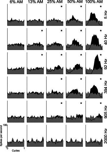
The period histograms are most modulated at high modulation depths. The lowest modulation depth at which significant modulation of the response occurs (*) varies with modulation frequency. At low- and high-modulation frequencies the response is less modulated than at the best modulation frequency (92 Hz). Primary-like unit, BF = 7.87 kHz, BMF = 92 Hz. Data shown were recorded in response to signals presented at 10 dB above pure-tone threshold. Grey shaded area indicates the response to an unmodulated pure tone. Black shaded area and think black line indicates the response to the modulated tone. Modulation depth is indicated at the top of each column. Modulation frequency is indicated to the right of each row. * in the top-right corner of each plot indicates significant phase-locking to the modulation frequency (P < 0.001, Rayleigh statistic > 13.8). Binwidth = 0.05 cycles.

Temporal modulation transfer functions were constructed from the VS of the period histograms (Fig. 2). These functions show the strength of temporal modulation in the spike train, in terms of the VS of spike phase locking to the stimulus modulation period (1/f_m), as a function of f_m and m. For all unit types, maximum VS decreases monotonically with decreasing m. The overall shape of the tMTF changes with unit type. Responses are classified as band-pass if the neural gain relative to the stimulus modulation decreases by 3 dB from the peak gain on both the upper and lower frequency edges of the tMTF. Similarly, responses are classified as low-pass if the neural gain decreases by 3 dB from the peak value on the upper frequency edge only. The shapes of the tMTFs are level dependent for all unit types. In general, PL units show a low-pass tMTF for the majority of stimulus conditions, whereas tMTFs recorded from CS units are typically band-pass. The tMTFs for CT units generally have a low-pass shape at 10 dB above pure-tone threshold, and become more band-pass at 40 dB above threshold; with m= 1, 73% (19/26) of the tMTFs are low-pass at 10 dB above pure-tone rate threshold, but 92% (24/26) are band-pass at 40 dB above threshold. A similar trend is seen in PL and in CS units. At 10 dB above threshold only 36% (4/11) of PL units’ tMTFs are classified as band-pass. This increased to 73% (8/11) at 40 dB above threshold. Similarly, at 10 dB above threshold 64% (9/14) of CS units’ tMTFs are band-pass, increasing to 100% (14/14) at 40 dB above threshold. Hence, there is a hierarchy in the tendency for units to be band-pass tuned in the modulation domain, CS>CT>PL.

Figure 2. Temporal modulation transfer functions as a function of modulation depth (m), sound level, and unit type.

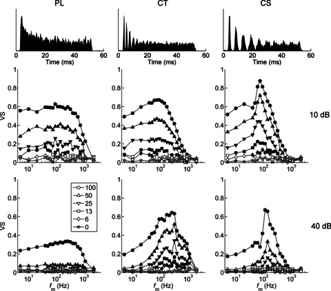
The PL unit has low-pass modulation transfer functions. The CT unit becomes more band-pass at the higher sound level. The CS unit is band-pass tuned at both low and high sound levels. Best modulation frequency does not change with modulation depth. Top row, peri-stimulus time histograms in response to 50 ms duration unmodulated BF tones. Middle row, tMTFs at 10 dB above pure-tone threshold. Bottom row, tMTFs at 40 dB above pure-tone threshold. VS, vector strength; f_m, modulation frequency.Left column, primary-like unit (BF = 7.87 kHz). Middle column, transient chopper unit (BF = 7.51 kHz). Right column, sustained chopper unit (BF = 8.15 kHz). Modulation depth (m, %) is shown in the key. Filled symbols are significant (P < 0.001, Rayleigh statistic > 13.8), and open symbols are non-significant.

As f_m is increased above BMF, VS decreases and becomes non-significant at the tMTF cut-off frequency (f_cut-off). The tMTF corner frequency (f_corner) is defined as the f_m at which the neural gain relative to the stimulus modulation is 3 dB lower than the gain at BMF for that m (see eqn. (4) in Methods). In the examples shown there is significant temporal modulation in the spike-train responses even for low modulation depths (Fig. 2). Both example chopper units (CT and CS) show significant representations of f_m over a narrow bandwidth for 6% AM at 10 dB above pure-tone threshold. At the higher stimulus presentation level, the lowest m at which the CS unit shows significant phase-locking to the amplitude envelope is 13%, whereas the CT unit maintains a significant representation of 6% AM. Therefore, in these examples the CT unit is more sensitive; i.e. has a lower (better) threshold for AM detection, than does the CS unit of a similar BF.

The majority of units have a BMF between approximately 50 and 300 Hz (Fig. 3A). For each unit type, increasing the presentation level from 10 to 40 dB above threshold significantly increases BMF (two-tailed paired Student's t tests, P < 0.01). Analysis of variance (ANOVA) indicates significant main effects of unit type and stimulus intensity on BMF (both P < 0.01). PL units have the highest mean BMF (172 and 296 Hz at 10 and 40 dB above pure-tone threshold, respectively). Mean BMFs are similar for CS and CT units (at 10 dB: 78 and 69 Hz, respectively; at 40 dB: 170 and 190 Hz, respectively). Post hoc comparisons (with Bonferroni correction for multiple comparisons) show that at both presentation levels the mean BMF of PL units is significantly higher than that of CT and CS units (all, P < 0.05).

Figure 3. Best modulation frequency (BMF), bandwidth, corner frequency (f_corner), and cut-off frequency (f_cut-off) as a function of unit best frequency (BF) for a population of PL, CT, and CS units.

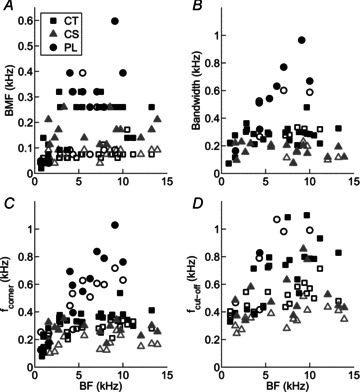
Open symbols indicate responses at 10 dB above pure-tone threshold, and filled symbols 40 dB above pure-tone threshold. Unit types as indicated in key in A. A, C and D, data from all tMTFs (low-pass and band-pass). B, data from band-pass tMTFs only.

Analysis of absolute bandwidths of band-pass tMTFs indicates a significant difference between unit types, with CS units having the sharpest tuning, followed by CT units, and PL units having the broadest tMTF tuning (Fig. 3B; ANOVA with post hoc Bonferroni correction for multiple comparisons, P < 0.05). However, after correcting for differences in BMF by expressing bandwidth as octaves relative to BMF (data not shown), there is no difference in the normalised tMTF bandwidth between unit types (ANOVA, P= 0.67). Normalised bandwidths are significantly narrower at 40 dB above threshold compared to 10 dB above threshold (ANOVA, P < 0.01). Corner frequency and f_cut-off are plotted as a function of BF for each unit type in the 100% AM condition in Fig. 3C and D, respectively. PL units have a significantly higher absolute f_corner compared to CT or CS units (both, P < 0.05), consistent with the data on absolute bandwidth, and the higher upper-limit of phase locking in PL units compared with CT and CS units (e.g. Winter & Palmer, 1990).

Features used to describe tMTFs, expressed relative to the 100%-AM condition are summarised as a function of m in Table 1. ANOVAs revealed that decreasing m: (i) has no significant effect on BMF (Table 1, P= 0.57), and (ii) leads to a significant decrease in tMTF bandwidth (Table 1, P < 0.01). This is consistent with the single-unit data presented in Fig. 2, showing a narrower range of f_m for which significant VS measurements were observed with decreasing m. As m decreases there is a significant decrease in f_corner across all unit types and presentation level combinations (Table 1, P < 0.01). The 10 dB cut-off frequency of the tMTF gain function decreases with m (Table 1, P < 0.01), and is significantly lower at 10 dB above pure-tone threshold compared to 40 dB above for each unit type (P < 0.01).

Table 1.

Effect of modulation depth on parameters of the temporal modulation transfer function Decreasing modulation depth is associated with significantly decreased tMTF bandwidth, corner frequency, and cut-off frequency. Best modulation frequency is independent of modulation depth. Data are expressed in octaves and as mean values (95% confidence interval), relative to that at m= 1. P value indicates the outcome of ANOVA. For analysis of the effect of modulation depth on bandwidth, only those tMTFs classified as ‘band-pass’ were included.

		Modulation depth, m
	Unit type	0.5	0.25	0.13	0.06	P
Δ BMF						0.57
	PL	−0.16	0.0	−0.07	−0.27
		[−0.72, 0.40]	[−0.43, 0.43]	[−0.53, 0.39]	[−0.72, 0.17]
	CT	−0.09	−0.11	−0.25	−0.26
		[−0.25, 0.07]	[−0.32, 0.11]	[−0.57, 0.07]	[−0.68, 0.16]
	CS	0.08	0.09	0.14	0.07
		[0.0, 0.15]	[0.0, 0.18]	[−0.01, 0.27]	[−0.12, 0.27]
Δ Bandwidth						< 0.01
	PL	−0.79	−0.66	–	–
		[−1.4, −0.18]	[−1.3, −0.06]
	CT	−0.45	−0.72	−0.77	−0.82
		[−0.64, −0.27]	[−1.0, −0.44]	[−1.12, −0.43]	[−1.3, −0.35]
	CS	−0.41	−0.55	−0.83	–
		[−0.54, −0.28]	[−0.70, −0.40]	[−1.2, −0.41]
Δfcorner						< 0.01
	PL	−0.30	−0.44	−0.82	−
		[−0.54, −0.07]	[−0.58, −0.32]	[−1.2, −0.44]
	CT	−0.30	−0.59	−0.86	−0.77
		[−0.40, −0.20]	[−0.73, −0.44]	[−1.1, −0.64]	[−1.1, −0.49]
	CS	−0.17	−0.24	−0.42	−0.41
		[−0.23, −0.11]	[−0.32, −0.17]	[−0.60, −0.23]	[−0.86, 0.05]
Δfcut-off						< 0.01
	PL	−0.27	−1.0	−1.5	−2.5
		[−0.56, 0.03]	[−1.5, −0.45]	[−2.1, −0.97]	[−3.0, −1.9]
	CT	−0.40	−1.1	−1.8	−2.3
		[−0.52, −0.29]	[−1.3, −0.81]	[−2.1, −1.4]	[−2.7, −1.9]
	CS	−0.40	−0.88	−1.5	−2.1
		[−0.55, −0.24]	[−1.0, −0.72]	[−1.7, −1.2]	[−2.3, −1.9]

Gain functions

From the measurements of VS we calculated the gain of the modulation in the neural response relative to the modulation in the stimulus. Single-unit data, showing the neural response modulation gain as a function of m for PL, CT, and CS units at 10 and 40 dB above pure-tone threshold, are plotted in Fig. 4. In general, neural response gain decreases monotonically with increasing m, and gain is lower at 40 dB above threshold compared to at 10 dB above threshold. Figure 5 shows the population mean gain, calculated from the significant portions of the tMTFs, as a function of normalised f_m relative to BMF. At 10 dB above pure-tone threshold, the gain functions of each unit type are largely positive. This indicates there is more modulation in the temporal response of the units than in the amplitude of the physical signal. The gain is greater for small m, indicating a compressive non-linearity in the stimulus–response transformation. At 40 dB above pure-tone threshold the gain is largely negative, with only those responses in a narrow frequency band centred on the BMF and at low m showing positive gain.

Figure 4. Modulation gain at BMF, as a function of modulation depth (m) and sound level, for a population of PL, CT, and CS units.

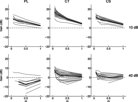
Gain decreases monotonically with increasing modulation depth and with increasing sound level. Grey lines, single-unit data. Black lines, population mean, calculated from the single-unit data. Top row, 10 dB above pure-tone threshold. Bottom row, 40 dB above pure-tone threshold. Dashed line in each plot indicates zero gain.

Figure 5. Modulation gain as a function of normalised modulation frequency (f_m), modulation depth (m) and sound level, for a population of PL, CT, and CS units.

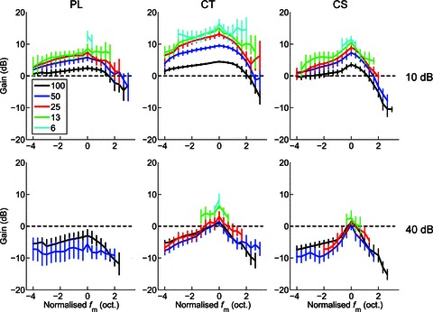
Gain increases with decreasing modulation depth (shown in key at top left, %). CT units show the highest gain, followed by CS units, and then PL units. Gain decreases (and becomes negative) with increasing sound level. Top row, at 10 dB above pure-tone rate threshold. Bottom row, at 40 dB above pure-tone threshold. Left column, primary-like (PL) responses. Middle column, transient chopper (CT) responses. Right column, sustained chopper (CS) responses. Dashed line indicates zero response modulation gain relative to the signal modulation. Data are population mean data calculated over significant portions of the tMTF (i.e. where Rayleigh > 13.8, P < 0.001). Error bars indicate 95% confidence intervals around the population mean.

ANOVA with the factors normalised f_m, m, unit type, and presentation level shows significant main effects of each factor on neural response modulation gain (ANOVA, all P < 0.01). Post hoc comparisons (with Bonferroni correction) show that at each m, the gain of CT units is significantly greater than that of either PL or CS units (all, P < 0.05). For each unit type, and at both presentation levels, the response gain did not differ between the 50% and 100% AM conditions (P > 0.05). Responses for all other values of m were significantly different within each unit type and presentation level combination, with smaller m giving significantly greater response modulation gain (P < 0.05).

Neurometric analysis

The analyses presented above allow a direct comparison of the data with previous studies of AM representation in the cochlear nucleus (Frisina et al. 1990a,b; Kim et al. 1990; Rhode, 1994). However, the purpose of the present study was to bridge the gap between physiological studies focusing on 100% AM and psychoacoustic studies examining the threshold for AM detection. Several studies at other auditory loci have used a neurometric approach to quantify the neural threshold for AM detection (Nelson & Carney, 2007; Yin et al. 2011; Johnson et al. 2012; Niwa et al. 2012). Using similar techniques (see Methods) we now turn our attention to a neurometric analysis of the VCN single unit data to determine the neural AM detection threshold at this level in the anaesthetised guinea-pig.

Figure 6 shows receiver operating characteristic (ROC) curves calculated from the responses of a single CT unit at seven different modulation frequencies and at each m between 6 and 100%. For each modulated stimulus condition, the VS_pp is compared to that calculated from the responses of the same unit to the 0% AM (i.e. unmodulated) stimulus condition with the same carrier frequency and sound level. The proportion of true positive (P_TP) and false positive (P_FP) signal classifications at each of 100 equally spaced decision criteria is plotted for each f_m–m combination. At low f_m (i.e. 5 Hz), the ROC curves for the 6% and 13% AM conditions are close to the chance level of 0.5 (dashed diagonal lines in plots in Figure 6). This indicates that at such low f_m, the responses of this unit to AM signals with low modulation depth are similar to the responses to an unmodulated signal. As f_m increases towards BMF, the area under the ROC curves increases, indicating that the responses to these signals become more discriminable from the responses to an unmodulated tone. As f_m is increased above BMF, the ROC curves become closer to 0.5, until at f_m= 905 Hz the ROC curves for all modulation-depth conditions (including 100% AM) lie close to chance performance.

Figure 6. Receiver operating characteristic (ROC) curves for a single unit as a function of modulation depth and modulation frequency at 10 dB above pure-tone threshold.

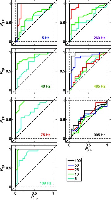
The signal becomes less discriminable from an unmodulated tone with decreasing modulation depth (see key at bottom right), and with both increasing and decreasing modulation frequency relative to best modulation frequency (139 Hz). Responses of a single CT unit (BF = 5.25 kHz), at 10 dB above pure-tone threshold. Probability of true positive (P_TP) AM detection plotted against the probability of false positive (P_FP) AM detection at 100 equally spaced decision criteria between 0 and the maximum phase-projected vector strength for each modulated–unmodulated signal combination. The modulation frequency corresponding to the modulated signal in each panel is indicated in the lower right-hand corner. The colour code of the text corresponds to values of f_m highlighted in Fig. 7. The colour code of the continuous lines corresponds to the modulation depth, as indicated in the figure legend. Diagonal dashed line indicates the expected value if the modulated signal were indistinguishable from an unmodulated tone on the basis of the phase-projected vector strength of spike synchrony at f_m.

From the ROC curves calculated from the responses of the single CT unit shown in Fig. 6, the area under the curve (AUC) of each function for each f_m–m combination was calculated. Mathematically the AUC corresponds to the probability of a randomly selected presentation of the modulated signal eliciting a VS_pp greater than a randomly selected presentation of the unmodulated signal. The AUC is plotted as a function of f_m at each m for the same single CT unit, in Fig. 7B. The corresponding tMTFs for this unit are plotted in Fig. 7A, with the data at selected f_m values highlighted in colour. These highlighted f_m conditions correspond to the ROC data plotted in Fig. 6. The AUC is maximal, at a value of 1.0, for the majority of f_m–m conditions. This indicates that an ideal observer would be able to discriminate the modulated from an unmodulated signal on the basis of these responses with 100% accuracy. At high f_m independent of m, and at low f_m at low m, the AUC decreases below 0.75, indicating that the modulated signal would be discriminated from an unmodulated signal on less than 75% of trials. Around the unit's BMF, the AUC for all modulation depth conditions is >0.75, so that even at the lowest modulation depth tested the unit's responses support correct identification of the modulated signal on >75% of trials.

Figure 7. Modulation-detection threshold is calculated as a function of modulation frequency.

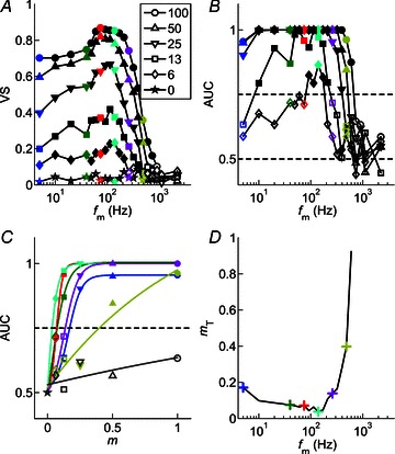
Logistic fits to the function relating the area under the ROC curve to modulation depth are used to determine the modulation depth at which the single unit response reaches threshold at each individual modulation frequency. The logistic function accurately describes the data. Threshold is lowest around the best modulation frequency, and increases with both increasing and decreasing f_m relative to best modulation frequency. Responses of a single CT unit (BF = 5.25 kHz), at 10 dB above pure-tone threshold. A, temporal modulation transfer functions calculated from the vector strength of spike synchrony to the amplitude envelope as a function of f_m and m, as indicated in the figure legend. Filled symbols represent significant VS measurements (Rayleigh statistic > 13.8, P < 0.001), open symbols indicate non-significant VS. Colours identify modulation frequencies (5, 40, 75, 139, 260, 485, 905 Hz) at which further analyses are presented in B–D. Key shows modulation depth (m, %).;B, area under the receiver operating characteristic curve (AUC) as a function of f_m and m. Dashed line at 0.5 indicates the expected value for a signal indistinguishable from an unmodulated signal. Dashed line at 0.75 indicates the value taken as threshold for AM detection. Filled symbols indicate values above threshold, open symbols indicate values below threshold. C, AUC plotted as a function of m for each of the modulation frequencies highlighted in colour in panels A and B. Continuous lines indicate logistic functions fitted to the data. Dashed line at 0.75 indicates threshold. Filled symbols indicate values above threshold, open symbols indicate values below threshold. The m value at which each fitted function crosses this dashed line is taken as the threshold modulation depth (m_T) for that f_m. D, neural threshold for AM detection plotted as a function of f_m calculated from the responses in A–C. Colours correspond to the modulation frequencies highlighted in A and B, and fitted with logistic functions in C. For this unit, minimum threshold for AM detection is 3.7% at f_m= 139 Hz. At f_m= 905 Hz, threshold is not reached at any m.

To determine the neural AM detection threshold we fitted the AUC as a function of m with logistic functions (see Methods). Figure 7C shows a group of fitted functions at each of the modulation frequencies highlighted in colour in Fig. 7A and B. The m value at which the fitted function reaches an AUC of 0.75 is taken as threshold for that f_m condition. At the highest f_m for which data are plotted (905 Hz), the data (and the fitted function) do not reach the threshold criterion level. For all other f_m conditions plotted, threshold is reached at a value of m which varies with f_m. Of the 2143 AUC vs. m plots, 1946 (90.8%) were successfully fitted with logistic functions as determined by the criteria set out in Methods (PL: 428/452, 94.7%; CT: 962/1059, 90.8%; CS: 556/632, 88%). The relationship between f_m and AM detection threshold (m_T) determined by this method is plotted for the same CT unit in Fig. 7D. Threshold is lowest (m≍ 3.7%) near BMF, and increases with both increasing and decreasing f_m relative to BMF. Threshold increases more rapidly on the high-frequency edge of the tMTF. From the single-unit data, the mean lowest threshold across the f_m-axis at 10 dB above pure-tone threshold for a population of 14 CS units is 5.8% (range, 2.6–10.6%; standard deviation (SD), 2.6%). For a population of 26 CT units the corresponding data are: mean, 6.5%; range, 1.3–21.9%; SD, 4.2%; for 11 PL units: mean, 7.3%; range, 4.1–13.8%; SD, 2.6%.

Figure 8 shows the mean ROC curves calculated from the responses of a population of PL, CT, and CS units for each m, at 10 (top row) and 40 dB (bottom row) above pure-tone threshold. The data in these plots are calculated from responses at the unit BMF. At m= 100% (black lines) the ROC curves for all unit types and at both presentation levels approach perfect performance; that is, the probability of a true positive is at or near 1 for all decision criteria levels. The diagonal dashed black lines in the plots in Fig. 8 indicate chance performance. As m is decreased the ROC curves approach chance-level performance. From the mean ROC curves in Fig. 8, the effect of decreasing m on the ability of single units to discriminate modulated signals from an unmodulated signal on the basis of temporal discharge patterns is greater at 40 dB than at 10 dB above pure-tone threshold; i.e. performance is worse at higher stimulus levels (ANOVA, P < 0.01).

Figure 8. Population mean receiver operating characteristic curves at the best modulation frequency for PL, CT, and CS units.

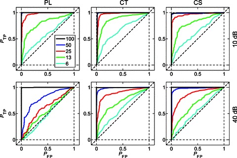
AM signals become less discriminable from unmodulated tones as modulation depth is decreased, and as sound level is increased. Top row, at 10 dB above pure-tone threshold. Bottom row, at 40 dB above pure-tone threshold. Left column, primary-like (PL) responses. Middle column, transient chopper (CT) responses. Right column, sustained chopper (CS) responses. The probability of a true positive (P_TP) AM signal detection is plotted against the probability of a false positive (P_FP) detection at each of 100 equally spaced decision criteria between 0 and the maximum phase-projected vector strength (VSpp) for the two signals being compared. The plotted functions are population mean data as a function of m as indicated in the key at top left. Diagonal dashed line indicates chance performance; i.e. the modulated signal is indiscriminable from an unmodulated tone.

The area under the ROC curves is plotted as a function of normalised f_m (i.e. octaves from BMF) and m for each unit type at both presentation levels in Fig. 9. At m= 100%, these functions are all low-pass in shape over the range of normalised f_m examined. Each unit type approaches perfect performance for values of f_m≤ BMF. In general, the functions become increasingly band-pass in shape as m is decreased. Single units are able to distinguish modulated from unmodulated signals over a smaller range of f_m around BMF as m is decreased. The population mean data for all unit types shows no significant discrimination for m < 13% at 10 dB above pure-tone threshold, and no significant discrimination for m < 25% for CT and CS units and for m < 50% for PL units at 40 dB above pure-tone threshold. ANOVA with the factors unit type, presentation level, m, and normalised f_m indicates significant main effects of each factor on the area under the ROC curves (all, P < 0.01).

Figure 9. Mean area under the receiver operating characteristic curves (AUC) as a function of normalised modulation frequency (f_m), modulation depth, and sound level, for a population of PL, CT, and CS units.

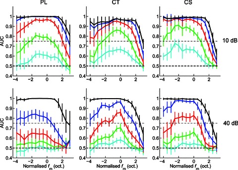
The area under the ROC curve decreases with decreasing modulation depth and with increasing sound level. This corresponds to a decreasing ability of neurons to discriminate between modulated and unmodulated signals by means of spike synchrony at f_m as modulation depth decreases, and as sound level increases. Colour key as in Fig. 8. Top row, at 10 dB above pure-tone threshold. Bottom row, at 40 dB above pure-tone threshold. Left column, primary-like (PL) responses. Middle column, transient chopper (CT) responses. Right column, sustained chopper (CS) responses. Dashed line at AUC = 0.5 indicates chance performance. Dashed line at AUC = 0.75 indicates threshold for AM detection (i.e. AUC significantly different from 0.5). Error bars indicate 95% confidence intervals around the population mean.

Figure 10 shows the population mean threshold for AM detection as a function of normalised f_m at both presentation levels for each unit type. In general, threshold for AM detection increases as f_m increases or decreases relative to BMF. The function relating threshold to normalised f_m becomes increasingly band-pass in shape as the presentation level is increased. ANOVA with the factors unit type, presentation level, and normalised f_m indicates significant main effects of each factor on threshold for AM detection (all, P < 0.01). Post hoc comparisons (with Bonferroni correction), indicate at both 10 dB and 40 dB above pure-tone threshold the AM detection threshold is significantly higher for PL units than for either CT or CS units (both, P < 0.05). Thresholds for CT and CS units are not significantly different at either presentation level. For each unit type threshold is significantly higher at 40 than at 10 dB above pure-tone threshold (P < 0.05).

Figure 10. Population mean amplitude-modulation detection threshold (m_T) as a function of normalised modulation frequency (f_m) and sound level for PL, CT and CS units.

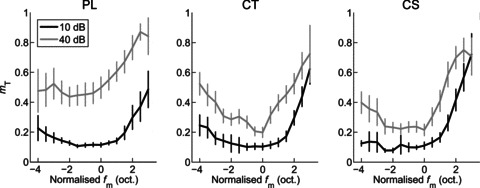
Threshold is lowest (i.e. best) around best modulation frequency (i.e. at normalised f_m= 0). Threshold worsens (i.e. increases) with both increasing and decreasing f_m relative to best modulation frequency, and with increasing sound level. The effect of sound level is greater for PL units than for CT or CS units. Left column, primary-like (PL) responses. Middle column, transient chopper (CT) responses. Right column, sustained chopper (CS) responses. Black lines, 10 dB above pure-tone threshold. Grey lines, 40 dB above pure-tone threshold. Error bars indicate 95% confidence intervals around the population mean.

Discussion

In this study we show that in the responses of single units in the ventral cochlear nucleus BMF is independent of modulation depth. In addition we show that neurometric AM detection threshold is best near to the best modulation frequency and varies with sound level and unit type. Chopper units have significantly better AM detection thresholds than do primary-like units, at both low and moderate sound levels.

Effect of modulation depth on neural tMTFs

The main effect of increasing m across all unit types tested (PL, CT, CS) is increased spike synchrony to f_m. This is reflected in the higher peak VS values in tMTFs. This effect has been noted in previous studies on AM representation in ANFs and CN units (Joris & Yin, 1992; Rhode, 1994). As m is increased from 6 to 100%, BMF remains constant. In contrast, as the stimulus level is increased from 10 to 40 dB above pure-tone threshold, BMF increases. Rhode (1994) provides the only previous report on the shape of neural tMTFs in VCN as a function of m. That report includes only two units with complete tMTFs plotted at three different values of m (0.5, 1.0, and 2.0; at m= 2.0, the three components of the acoustic signal are equal amplitude). The BMFs determined at m= 0.5 and 1.0 from Rhode's Fig. 10D (unit classified as CS), are also equal. Rhode (1994) shows VS measurements from a population of VCN units as a function of m at BMF. VS increased monotonically with increasing m for all unit types, as is the case with the present data. However, it is not clear from the Rhode's data at which value of m spike synchronisation becomes significantly different from that which would be observed by chance in response to an unmodulated signal.

Similar to previous reports, our data show a change in the overall shape of the tMTF with presentation level and unit type (Frisina et al. 1990a; Rhode, 1994; Rhode & Greenberg, 1994). PL units show a low-pass response for the majority of stimulus conditions, whereas tMTFs recorded from CS units are typically band-pass. CT units’ tMTFs are generally low-pass in shape at 10 dB above pure-tone threshold, and become more band-pass at 40 dB above threshold. As m is decreased the corner frequency, cut-off frequency, and bandwidth of tMTFs decrease. This indicates the bandwidth of f_m around the BMF within which the unit can convey a significant temporal representation of AM decreases with decreasing m in a predictable and consistent manner. The decreased bandwidth of the significant portion of the tMTF is also reflected in the gain functions plotted in Fig. 5. At low m, the gain of the response modulation relative to the signal modulation is significantly higher than at higher values of m. However, the bandwidth over which this is the case is decreased; indicating a sharpening of tuning in the modulation domain at low m across the VCN. The effect is more pronounced at the higher presentation level.

The interaction of the spectrum of the AM signal and the ‘V-shaped’ filter (in frequency-level coordinates) of peripheral auditory neurons is an important consideration in understanding the effects of modulation depth on AM representation. As m is decreased, the level of the side bands at f_c+f_m and at f_c–f_m decreases by 6 dB for each halving of m. The side bands gradually fall out of the filter as they decrease in level, and therefore it would be expected that any temporal response at f_m would cease when there is no longer a side band interacting with the f_c component within the filter. However, in ANF recordings, by comparing the effect on neural synchrony to f_m of decreasing m with that of increasing f_m, Joris & Yin (1992) showed the attenuation of modulation side bands by peripheral filtering alone does not account for the decrease in neural synchrony to f_m. Our results indicate significant spike synchronisation at low f_m even when the side bands are below spike rate threshold. For example, in Fig. 2 there are significant responses from a CS unit with f_m in the region of 100 Hz, at m= 6% for signals 10 dB above audio-visual spike rate threshold. At this modulation depth the side bands of the three-component AM signal are 30 dB lower in level than the on-BF f_c component; i.e. the side bands are 20 dB below BF spike rate threshold. Joris & Yin (1992) show similar results in ANFs (their Fig. 3). It is known that spike synchrony threshold is approximately 20 dB lower than spike rate threshold in the auditory nerve (Johnson, 1980). In their study of AM detection and discrimination threshold Nelson & Carney (2007) show detection thresholds based on synchronisation are lower than those based on changes in mean spike rate.

Level dependence

Amplitude-modulation detection threshold, as calculated from the temporal responses of VCN PL, CT, and CS units, is dependent on signal presentation level (Fig. 8). PL units show the greatest level dependence, with thresholds increased from m of ∼10 to ∼40% at BMF as presentation level is increased from 10 to 40 dB above pure-tone threshold. CT and CS units are less sensitive to changes in presentation level, with AM detection thresholds of ∼10 and ∼22% at 10 and 40 dB above pure-tone threshold, respectively. Psychoacoustic AM detection thresholds using a wideband-noise carrier are largely level in dependent at sensation levels of 20 dB and above (Viemeister, 1979). The observed neurometric threshold level dependence is somewhat at odds with the results of some human psychoacoustic experiments. With tone or narrowband noise carriers, psychoacoustic thresholds are level dependent, but in the opposite direction to that seen here; thresholds decrease (i.e. improve) with increasing sound level (Kohlrausch, 1993; Kohlrausch et al. 2000).

This observation of improved behavioural detection thresholds with increasing sound level is difficult to explain on the basis of a spike-synchrony model in VCN single units. However, as shown in Fig. 2, it is well-established that the VS of spike synchrony to the amplitude envelope in CN units decreases with increasing sound level (Rhode, 1994; Rhode & Greenberg, 1994; Joris et al. 2004). Similar decreases in spike synchrony to AM tones with increasing sound level are also observed in ANF responses (e.g. Dreyer & Delgutte, 2006). The effect of changes in sound level on the responses to AM signals in IC units is more complex (Krishna & Semple, 2000; Nelson & Carney, 2007). The increased sensitivity to AM with increased presentation level for narrow-band carriers has been hypothesised to reflect a spread of excitation to a larger number of neurons across the BF axis with increasing sound level. This would be equivalent to the increased sensitivity of an ‘across-cell pooling’ mechanism invoked to account for psychoacoustic AM detection thresholds based on cortical responses (e.g. Johnson et al. 2012).

Comparisons between neurometric and psychometric thresholds

Human psychoacoustic experiments have demonstrated exquisite sensitivity to AM (Viemeister, 1973, 1979; Sheft & Yost, 1990; Lee & Bacon, 1997; Kohlrausch et al. 2000). Over the most sensitive range of f_m (<∼50–100 Hz), human AM detection thresholds are approximately 5–10% for AM wideband noise, and 3–5% for AM tones. Guinea-pig behavioural data are not available for direct comparison with the neural data. However, there are a number of studies relevant for a comparison of behaviour with physiology. Behavioural AM detection thresholds have been studied in several non-human mammalian and avian species (Fay, 1980; Salvi et al. 1982; Dooling & Searcy, 1985; Klump & Okanoya, 1991; Kelly et al. 2006; Wiegrebe & Sonnleitner, 2007; O’Connor et al. 2011). In general, AM detection thresholds are approximately 5% points higher at low f_m (<∼50 Hz) in non-humans compared to humans. At higher f_m, thresholds are similar across species (Klump & Okanoya, 1991).

Recent primate studies have shown close correspondence of both spike-rate-based and spike-synchrony-based measures of AM detection threshold in auditory cortex, with those measured behaviourally in the same species (O’Connor et al. 2011; Yin et al. 2011; Johnson et al. 2012; Niwa et al. 2012). The closest correspondence of neurometric to psychometric thresholds was achieved with a weighted across-cell pooling of responses (Johnson et al. 2012). The mean neural AM detection thresholds in the same study were approximately 10–20% higher than behavioural thresholds, and the most sensitive neurons out-performed (i.e. lower (better) threshold) the whole animal on both rate-based and synchrony-based measures. At a cortical level, attention improved both spike-rate-based and spike-synchrony-based thresholds for AM detection (Niwa et al. 2012). Similar to these studies in monkeys, but at the opposite end of the auditory nervous system, previous authors have compared behavioural AM detection thresholds with physiological AM detection thresholds calculated from ANF recordings in the European Starling (Klump & Okanoya, 1991; Gleich & Klump, 1995). Using a spike-synchrony analysis akin to that used in the present study, Klump's group found the average ANF sensitivity to AM was ∼ 20% less than that determined behaviourally (i.e. thresholds were 20% worse in the ANFs), over the f_m range 5–1280 Hz. However, the most sensitive ANFs in their study had thresholds approaching those determined behaviourally.

The IC has been studied extensively with regard to AM coding (e.g. Rees & Møller, 1983; Langner & Schreiner, 1988; Rees & Palmer, 1989; Krishna & Semple, 2000; Nelson & Carney, 2007; Borina et al. 2008). IC neurons change their responses with variations in f_m and m. Some IC units show spike-rate-based band-pass MTFs, some units show spike-synchrony-based modulation tuning with band-pass or low-pass tMTFs, and some show spike-rate and spike-synchrony tuning (Langner & Schreiner, 1988; Joris et al. 2004). In general, it is thought the IC plays a transitional role between synchrony-based representations of AM in the periphery and more rate-based representations in central loci (Langner, 1992; Nelson & Carney, 2007). In their study of AM detection and discrimination threshold, Nelson & Carney (2007) showed neural synchronisation to the amplitude envelope of tone carriers can accurately predict behavioural AM detection threshold. While a spike-rate-based metric was a poor predictor of AM detection threshold, spike rate accounted for AM depth discrimination in some neurons.

Auditory nerve fibres, IC neurons, and auditory cortical neurons can each account for the perceptual threshold of AM detection by varying their firing rate or temporal discharge pattern in response to changes in m. Thresholds determined in this study for guinea-pig VCN neurons on the basis of spike synchrony are less variable than those in the primary auditory cortex of awake non-behaving macaque monkeys (Johnson et al. 2012). Comparing the present guinea-pig data to behavioural AM detection thresholds determined with 20 kHz-wide AM noise in the chinchilla (Salvi et al. 1982), we find a close relationship between the mean neural data at 10 dB above threshold and these behavioural thresholds. For f_m < ∼100Hz, Salvi et al. (1982) find thresholds of approximately 10%. This increases to approximately 40% at f_m in the region of 2 kHz. For the guinea-pig VCN (PL, CT, and CS units), at 10 dB above pure-tone threshold, neural AM detection threshold is in the region of 10% at BMF, and for two octaves below BMF. This is based on a population of units with BMFs in the range 40–600 Hz. For f_m above BMF, threshold increases to approximately 40% at two octaves above BMF (Fig. 10). Therefore there is close correspondence between the average VCN neurometric AM detection thresholds and those measured behaviourally in the chinchilla. The most sensitive individual neurons out-perform these whole animal measurements. How the output of individual VCN neurons (or, in fact, any neuron) is combined by a central processor to result in perception is as yet unknown, making the interpretation of the relationship between a single neuron's response and a whole animal's behaviour difficult. Neuronal pooling models have been successful in explaining psychophysical results in both the visual and auditory systems (Shadlen et al. 1996; Bizley et al. 2010; Johnson et al. 2012). The average response of a population of neurons may be thought of as a form of neural pooling. However, the ‘response’ of an individual neuron in neurophysiological studies is usually the result of averaging across many stimulus presentations, simulating the average response of many neurons. Even a single presentation of an AM signal includes averaging of the neural response across multiple modulation cycles in the period histogram.

While previous studies have ascribed AM detection and the use of AM in perceptual tasks to activity in auditory cortical neurons (Liang et al. 2002; Johnson et al. 2012; Niwa et al. 2012), it must be remembered that vertebrate species lacking a true neocortex can detect AM signals using more primitive auditory nervous systems based on brainstem structures alone (Fay, 1980; Dooling & Searcy, 1985; Klump & Okanoya, 1991). Previous data from this laboratory have shown that neurometric functions in guinea-pig VCN accurately predict human psychophysical performance on a perceptual streaming task (Pressnitzer et al. 2008). Therefore, the contribution of brainstem neural thresholds for AM detection to animal behavioural thresholds should not be discounted. Neither should the correspondence between brainstem neural thresholds and psychoacoustic thresholds be taken as evidence for more central loci having no role in AM detection. It is possible that perceptual tasks involving AM detection recruit a distributed neural network involving cortical and subcortical processes. Such mechanisms may be an efficient means of processing information, not only for audition but across sensory modalities (Leopold & Maier, 2006).

It must also be borne in mind that the majority of physiological studies of AM processing, including this one, are performed under anaesthesia. The central auditory system contains descending projections from the cortex to most brainstem nuclei, including the cochlear nucleus, and from the midbrain to the cochlea itself; the olivo-cochlear bundle. Whether these projections are active (or if active, functional) under anaesthesia remains an open question. However, there are only a few isolated reports of the effects of anaesthesia on VCN responses (e.g. May & Sachs, 1992) making it difficult to speculate further on the effects of anaesthesia on VCN responses to AM signals. Even in neurophysiological studies of AM processing in awake primates there are large differences in AM discrimination thresholds when comparing passive to active listening conditions (Niwa et al. 2012). So anaesthesia alone may not be the only limiting factor in the interpretation of these data; behavioural state may be important too.

Models of amplitude modulation detection

Physiologically inspired models of AM coding in the auditory system have been heavily influenced by the finding of rate-tuned modulation filters in the responses of neurons in the inferior colliculus (Langner & Schreiner, 1988; Hewitt & Meddis, 1994). Such models envisage ‘coincidence-detector’ IC neurons receiving convergent input from a group of CN units. In one model (Hewitt & Meddis, 1994), the IC units receive their convergent input from a group of VCN CS units with similar BMFs. When the stimulus f_m periodicity matches the BMF of the CS units, synchrony will be maximal, resulting in a peak in the firing rate of the target IC unit. Some authors have found a correlation between the BMF of chopper units and their intrinsic oscillation frequency (Kim et al. 1990; Winter et al. 2001). However, other data does not support this assertion (Frisina et al. 1990a,b). For this model of AM coding to be physiological plausible, intrinsic oscillation frequencies (and BMFs) covering the range of AM perception is required (i.e. chopping periods of up to tens of milliseconds). There is little evidence for the required range of chopper unit BMFs over the entire BF range. In fact, the majority of chopper units have a BMF between 100 and 400 Hz (e.g. Kim et al. 1990). Alternative models propose that AM related information is processed in a circuit involving the projection of VCN bushy cells (PL units) to IC, with the circuit involving convergence of long-duration inhibition and short-duration excitation (Nelson & Carney, 2004). The present study provides useful information on an additional physiological parameter, m, to aid the design of computational models for the understanding of the neural coding of simple AM signals, and of signals with complex amplitude-modulation spectra, such as speech.

Glossary

AM

amplitude modulation

AN

auditory nerve

ANF

auditory nerve fibre

BF

best frequency

BMF

best modulation frequency

CAP

compound action potential

CN

cochlear nucleus

CS

sustained chopper

CT

transient chopper

f_m

modulation frequency

IC

inferior colliculus

PL

primary-like

ROC

receiver operating characteristic

RS

Rayleigh statistic

tMTF

temporal modulation transfer function

VCN

ventral cochlear nucleus

VS

vector strength

Additional information

Competing interests

None.

Author contributions

M.S., C.F., and I.M.W. designed the experiments and collected the data. M.S. wrote the MATLAB analysis programs, analysed the data, and wrote the manuscript. All authors edited the manuscript for important intellectual content and approved the final version of the manuscript. All experiments were performed at the Centre for the Neural Basis of Hearing, The Physiological Laboratory, Department of Physiology, Development and Neuroscience, University of Cambridge.

Funding

This project was funded by grants to I.M.W. from the BBSRC. M.S. received funding from the Frank Edward Elmore fund of the Cambridge MB/PhD programme, and from the Leatherseller's company, London. C.F. was funded by a Marie-Curie Intra-European Fellowship, and a Wolfson College (Cambridge) Junior Research Fellowship.

References

- Bizley JK, Walker KM, King AJ, Schnupp JW. Neural ensemble codes for stimulus periodicity in auditory cortex. J Neurosci. 2010;30:5078–5091. doi: 10.1523/JNEUROSCI.5475-09.2010. [DOI] [PMC free article] [PubMed] [Google Scholar]
- Blackburn CC, Sachs MB. Classification of unit types in the anteroventral cochlear nucleus: PST histograms and regularity analysis. J Neurophysiol. 1989;62:1303–1329. doi: 10.1152/jn.1989.62.6.1303. [DOI] [PubMed] [Google Scholar]
- Borina F, Firzlaff U, Schuller G, Wiegrebe L. Representation of echo roughness and its relationship to amplitude-modulation processing in the bat auditory midbrain. Eur J Neurosci. 2008;27:2724–2732. doi: 10.1111/j.1460-9568.2008.06247.x. [DOI] [PubMed] [Google Scholar]
- Bregman AS. Auditory Scene Analysis. Cambridge, MA, USA: MIT Press; 1990. [Google Scholar]
- Burns EM, Viemeister N. Nonspectral pitch. J Acoust Soc Am. 1976;60:863–869. [Google Scholar]
- Burns EM, Viemeister N. Played again SAM: Futher observations on the pitch of amplitude-modulated noise. J Acoust Soc Am. 1981;70:1655–1660. [Google Scholar]
- Colletti L, Shannon R, Colletti V. Auditory brainstem implants for neurofibromatosis type 2. Curr Opin Otolaryngol Head Neck Surg. 2012;20:353–357. doi: 10.1097/MOO.0b013e328357613d. [DOI] [PubMed] [Google Scholar]
- DiMattina C, Wang X. Virtual vocalization stimuli for investigating neural representations of species–specific vocalizations. J Neurophysiol. 2006;95:1244–1262. doi: 10.1152/jn.00818.2005. [DOI] [PubMed] [Google Scholar]
- Dollezal LV, Beutelmann R, Klump GM. Stream segregation in the perception of sinusoidally amplitude-modulated tones. PLoS One. 2012;7:e43615. doi: 10.1371/journal.pone.0043615. [DOI] [PMC free article] [PubMed] [Google Scholar]
- Dooling RJ, Searcy MH. Temporal integration of acoustic signals by the budgerigar (Melopsittacus undulatus. J Acoust Soc Am. 1985;77:1917–1920. doi: 10.1121/1.391835. [DOI] [PubMed] [Google Scholar]
- Dreyer A, Delgutte B. Phase locking of auditory-nerve fibers to the envelopes of high-frequency sounds: implications for sound localization. J Neurophysiol. 2006;96:2327–2341. doi: 10.1152/jn.00326.2006. [DOI] [PMC free article] [PubMed] [Google Scholar]
- Fay RR. Psychophysics and neurophysiology of temporal factors in hearing by the goldfish: amplitude modulation detection. J Neurophysiol. 1980;44:312–332. doi: 10.1152/jn.1980.44.2.312. [DOI] [PubMed] [Google Scholar]
- Fishman YI, Volkov IO, Noh MD, Garell PC, Bakken H, Arezzo JC, Howard MA, Steinschneider M. Consonance and dissonance of musical chords: neural correlates in auditory cortex of monkeys and humans. J Neurophysiol. 2001;86:2761–2788. doi: 10.1152/jn.2001.86.6.2761. [DOI] [PubMed] [Google Scholar]
- Frisina RD, Smith RL, Chamberlain SC. Encoding of amplitude modulation in the gerbil cochlear nucleus: I. A hierarchy of enhancement. Hear Res. 1990a;44:99–122. doi: 10.1016/0378-5955(90)90074-y. [DOI] [PubMed] [Google Scholar]
- Frisina RD, Smith RL, Chamberlain SC. Encoding of amplitude modulation in the gerbil cochlear nucleus: II. Possible neural mechanisms. Hear Res. 1990b;44:123–142. doi: 10.1016/0378-5955(90)90075-z. [DOI] [PubMed] [Google Scholar]
- Gleich O, Klump GM. Temporal modulation transfer functions in the European Starling (Sturnus vulgaris): II. Responses of auditory-nerve fibres. Hear Res. 1995;82:81–92. doi: 10.1016/0378-5955(94)00168-p. [DOI] [PubMed] [Google Scholar]
- Goldberg JM, Brown PB. Responses of binaural neurons in the dog superior olivary complex to dichotic stimuli: Some physiological mechanisms of sound localization. J Neurophysiol. 1969;32:613–636. doi: 10.1152/jn.1969.32.4.613. [DOI] [PubMed] [Google Scholar]
- Green DM, Swets JA. Signal Detection Theory and Psychophysics. New York: Wiley; 1966. [Google Scholar]
- Grimault N, Bacon SP, Micheyl C. Auditory stream segregation on the basis of amplitude-modulation rate. J Acoust Soc Am. 2002;111:1340–1348. doi: 10.1121/1.1452740. [DOI] [PubMed] [Google Scholar]
- Hewitt MJ, Meddis R. A computer model of amplitude-modulation sensitivity of single units in the inferior colliculus. J Acoust Soc Am. 1994;95:2145–2159. doi: 10.1121/1.408676. [DOI] [PubMed] [Google Scholar]
- Johnson DH. The relationship between spike rate and synchrony in responses of auditory-nerve fibers to single tones. J Acoust Soc Am. 1980;68:1115–1122. doi: 10.1121/1.384982. [DOI] [PubMed] [Google Scholar]
- Johnson JS, Yin P, O’Connor KN, Sutter ML. Ability of primary auditory cortical neurons to detect amplitude modulation with rate and temporal codes: neurometric analysis. J Neurophysiol. 2012;107:3325–3341. doi: 10.1152/jn.00812.2011. [DOI] [PMC free article] [PubMed] [Google Scholar]
- Joris PX, Schreiner CE, Rees A. Neural processing of amplitude-modulated sounds. Physiol Rev. 2004;84:541–577. doi: 10.1152/physrev.00029.2003. [DOI] [PubMed] [Google Scholar]
- Joris PX, Yin TC. Responses to amplitude-modulated tones in the auditory nerve of the cat. J Acoust Soc Am. 1992;91:215–232. doi: 10.1121/1.402757. [DOI] [PubMed] [Google Scholar]
- Kelly JB, Cooke JE, Gilbride PC, Mitchell C, Zhang H. Behavioral limits of auditory temporal resolution in the rat: amplitude modulation and duration discrimination. J Comp Psychol. 2006;120:98–105. doi: 10.1037/0735-7036.120.2.98. [DOI] [PubMed] [Google Scholar]
- Kim DO, Sirianni JG, Chang SO. Responses of DCN-PVCN neurons and auditory nerve fibers in unanaesthetized decerebrate cats to AM and pure tones: Analysis with autocorrelation/power spectrum. Hear Res. 1990;45:95–113. doi: 10.1016/0378-5955(90)90186-s. [DOI] [PubMed] [Google Scholar]
- Klump GM, Okanoya K. Temporal modulation transfer functions in the European starling (Sturnus vulgaris): I. Psychophysical modulation detection thresholds. Hear Res. 1991;52:1–11. doi: 10.1016/0378-5955(91)90182-9. [DOI] [PubMed] [Google Scholar]
- Kohlrausch A. Comment on “Temporal modulation transfer functions in patients with cochlear implants”[J. Acoust. Soc. Am. 91,2156–2164 (1992)] J Acoust Soc Am. 1993;93:1649–1652. doi: 10.1121/1.406826. [DOI] [PubMed] [Google Scholar]
- Kohlrausch A, Fassel R, Dau T. The influence of carrier level and frequency on modulation and beat-detection thresholds for sinusoidal carriers. J Acoust Soc Am. 2000;108:723–734. doi: 10.1121/1.429605. [DOI] [PubMed] [Google Scholar]
- Krishna BS, Semple MN. Auditory temporal processing: responses to sinusoidally amplitude-modulated tones in the inferior colliculus. J Neurophysiol. 2000;84:255–273. doi: 10.1152/jn.2000.84.1.255. [DOI] [PubMed] [Google Scholar]
- Langner G. Periodicity coding in the auditory-system. Hear Res. 1992;60:115–142. doi: 10.1016/0378-5955(92)90015-f. [DOI] [PubMed] [Google Scholar]
- Langner G, Albert M, Briede T. Temporal and spatial coding of periodicity information in the inferior colliculus of awake chinchilla (Chinchilla laniger. Hear Res. 2002;168:110–130. doi: 10.1016/s0378-5955(02)00367-2. [DOI] [PubMed] [Google Scholar]
- Langner G, Schreiner CE. Periodicity coding in the inferior colliculus of the cat. I. Neuronal mechanisms. J Neurophysiol. 1988;60:1799–1822. doi: 10.1152/jn.1988.60.6.1799. [DOI] [PubMed] [Google Scholar]
- Lee J, Bacon SP. Amplitude modulation depth discrimination of a sinusoidal carrier: effect of stimulus duration. J Acoust Soc Am. 1997;101:3688–3693. doi: 10.1121/1.418329. [DOI] [PMC free article] [PubMed] [Google Scholar]
- Leopold DA, Maier A. Neuroimaging: perception at the brain's core. Curr Biol. 2006;16:R95–98. doi: 10.1016/j.cub.2006.01.026. [DOI] [PubMed] [Google Scholar]
- Liang L, Lu T, Wang X. Neural representations of sinusoidal amplitude and frequency modulations in the primary auditory cortex of awake primates. J Neurophysiol. 2002;87:2237–2261. doi: 10.1152/jn.2002.87.5.2237. [DOI] [PubMed] [Google Scholar]
- Mardia KV, Jupp P. Directional Statistics. New York: Wiley; 2000. [Google Scholar]
- May BJ, Sachs MB. Dynamic range of neural rate responses in the ventral cochlear nucleus of awake cats. J Neurophysiol. 1992;68:1589–1602. doi: 10.1152/jn.1992.68.5.1589. [DOI] [PubMed] [Google Scholar]
- Merrill EG, Ainsworth A. Glass-coated platinum-plated tungsten microelectrodes. Med Biol Eng. 1972;10:662–672. doi: 10.1007/BF02476084. [DOI] [PubMed] [Google Scholar]
- Middlebrooks JC. Auditory cortex phase locking to amplitude-modulated cochlear implant pulse trains. J Neurophysiol. 2008;100:76–91. doi: 10.1152/jn.01109.2007. [DOI] [PMC free article] [PubMed] [Google Scholar]
- Nelken I, Rotman Y, Bar Yosef O. Responses of auditory-cortex neurons to structural features of natural sounds. Nature. 1999;397:154–157. doi: 10.1038/16456. [DOI] [PubMed] [Google Scholar]
- Nelson PC, Carney LH. A phenomenological model of peripheral and central neural responses to amplitude-modulated tones. J Acoust Soc Am. 2004;116:2173–2186. doi: 10.1121/1.1784442. [DOI] [PMC free article] [PubMed] [Google Scholar]
- Nelson PC, Carney LH. Neural rate and timing cues for detection and discrimination of amplitude-modulated tones in the awake rabbit inferior colliculus. J Neurophysiol. 2007;97:522–539. doi: 10.1152/jn.00776.2006.. [DOI] [PMC free article] [PubMed] [Google Scholar]
- Niwa M, Johnson JS, O’Connor KN, Sutter ML. Active engagement improves primary auditory cortical neurons’ ability to discriminate temporal modulation. J Neurosci. 2012;32:9323–9334. doi: 10.1523/JNEUROSCI.5832-11.2012. [DOI] [PMC free article] [PubMed] [Google Scholar]
- O’Connor KN, Johnson JS, Niwa M, Noriega NC, Marshall EA, Sutter ML. Amplitude modulation detection as a function of modulation frequency and stimulus duration: comparisons between macaques and humans. Hear Res. 2011;277:37–43. doi: 10.1016/j.heares.2011.03.014. [DOI] [PMC free article] [PubMed] [Google Scholar]
- Pressnitzer D, Sayles M, Micheyl C, Winter IM. Perceptual organization of sound begins in the auditory periphery. Curr Biol. 2008;18:1124–1128. doi: 10.1016/j.cub.2008.06.053. [DOI] [PMC free article] [PubMed] [Google Scholar]
- Rees A, Møller AR. Responses of neurons in the inferior colliculus of the rat to AM and FM tones. Hear Res. 1983;10:301–330. doi: 10.1016/0378-5955(83)90095-3. [DOI] [PubMed] [Google Scholar]
- Rees A, Palmer AR. Neuronal responses to amplitude-modulated and pure-tone stimuli in the guinea pig inferior colliculus, and their modification by broadband noise. J Acoust Soc Am. 1989;85:1978–1994. doi: 10.1121/1.397851. [DOI] [PubMed] [Google Scholar]
- Rhode WS. Temporal coding of 200% amplitude modulated signals in the ventral cochlear nucleus of cat. Hear Res. 1994;77:43–68. doi: 10.1016/0378-5955(94)90252-6. [DOI] [PubMed] [Google Scholar]
- Rhode WS, Greenberg S. Encoding of amplitude modulation in the cochlear nucleus of the cat. J Neurophysiol. 1994;71:1797–1825. doi: 10.1152/jn.1994.71.5.1797. [DOI] [PubMed] [Google Scholar]
- Rhode WS, Roth GL, Recio-Spinoso A. Response properties of cochlear nucleus neurons in monkeys. Hear Res. 2010;259:1–15. doi: 10.1016/j.heares.2009.06.004. [DOI] [PMC free article] [PubMed] [Google Scholar]
- Salvi RJ, Giraudi DM, Henderson D, Hamernik RP. Detection of sinusoidally amplitude modulated noise by the chinchilla. J Acoust Soc Am. 1982;71:424–429. doi: 10.1121/1.387445. [DOI] [PubMed] [Google Scholar]
- Sayles M, Winter IM. Reverberation challenges the temporal representation of the pitch of complex sounds. Neuron. 2008;58:789–801. doi: 10.1016/j.neuron.2008.03.029. [DOI] [PubMed] [Google Scholar]
- Shadlen MN, Britten KH, Newsome WT, Movshon JA. A computational analysis of the relationship between neuronal and behavioral responses to visual motion. J Neurosci. 1996;16:1486–1510. doi: 10.1523/JNEUROSCI.16-04-01486.1996. [DOI] [PMC free article] [PubMed] [Google Scholar]
- Shannon RV, Zeng FG, Kamath V, Wygonski J, Ekelid M. Speech recognition with primarily temporal cues. Science. 1995;270:303–304. doi: 10.1126/science.270.5234.303. [DOI] [PubMed] [Google Scholar]
- Sheft S, Yost WA. Temporal integration in amplitude modulation detection. J Acoust Soc Am. 1990;88:796–805. doi: 10.1121/1.399729. [DOI] [PubMed] [Google Scholar]
- Singh NC, Theunissen FE. Modulation spectra of natural sounds and ethological theories of auditory processing. J Acoust Soc Am. 2003;114:3394–3411. doi: 10.1121/1.1624067. [DOI] [PubMed] [Google Scholar]
- Verhey JL, Pressnitzer D, Winter IM. The psychophysics and physiology of comodulation masking release. Exp Brain Res. 2003;153:405–417. doi: 10.1007/s00221-003-1607-1. [DOI] [PubMed] [Google Scholar]
- Viemeister N. Temporal modulation transfer functions based upon modulation thresholds. J Acoust Soc Am. 1979;66:1364–1380. doi: 10.1121/1.383531. [DOI] [PubMed] [Google Scholar]
- Viemeister NF. Temporal modulation transfer functions for audition. J Acoust Soc Am. 1973;53:512. doi: 10.1121/1.383531. [DOI] [PubMed] [Google Scholar]
- Wiegrebe L, Sonnleitner V. Perceptual interaction between carrier periodicity and amplitude-modulation in the gerbil (Meriones unguiculatus. J Comp Physiol A Neuroethol Sens Neural Behav Physiol. 2007;193:305–312. doi: 10.1007/s00359-006-0188-4. [DOI] [PubMed] [Google Scholar]
- Winter IM, Palmer AR. Responses of single units in the anteroventral cochlear nucleus of the guinea pig. Hear Res. 1990;44:161–178. doi: 10.1016/0378-5955(90)90078-4. [DOI] [PubMed] [Google Scholar]
- Winter IM, Wiegrebe L, Patterson RD. The temporal representation of the delay of iterated rippled noise in the ventral cochlear nucleus of the guinea-pig. J Physiol. 2001;537:553–566. doi: 10.1111/j.1469-7793.2001.00553.x. [DOI] [PMC free article] [PubMed] [Google Scholar]
- Yin P, Johnson JS, O’Connor KN, Sutter ML. Coding of amplitude modulation in primary auditory cortex. J Neurophysiol. 2011;105:582–600. doi: 10.1152/jn.00621.2010. [DOI] [PMC free article] [PubMed] [Google Scholar]
- Young ED, Robert JM, Shofner WP. Regularity and latency of units in the ventral cochlear nucleus: implications for unit classification and generation of response properties. J Neurophysiol. 1988;60:1–29. doi: 10.1152/jn.1988.60.1.1. [DOI] [PubMed] [Google Scholar]