A geometric framework for evaluating rare variant tests of association

Abstract

The wave of next-generation sequencing data has arrived. However, many questions still remain about how to best analyze sequence data, particularly the contribution of rare genetic variants to human disease. Numerous statistical methods have been proposed to aggregate association signals across multiple rare variant sites in an effort to increase statistical power; however, the precise relation between the tests is often not well understood. We present a geometric representation for rare variant data in which rare allele counts in case and control samples are treated as vectors in Euclidean space. The geometric framework facilitates a rigorous classification of existing rare variant tests into two broad categories: tests for a difference in the lengths of the case and control vectors, and joint tests for a difference in either the lengths or angles of the two vectors. We demonstrate that genetic architecture of a trait, including the number and frequency of risk alleles, directly relates to the behavior of the length and joint tests. Hence, the geometric framework allows prediction of which tests will perform best under different disease models. Furthermore, the structure of the geometric framework immediately suggests additional classes and types of rare variant tests. We consider two general classes of tests which show robustness to non-causal and protective variants. The geometric framework introduces a novel and unique method to assess current rare variant methodology and provides guidelines for both applied and theoretical researchers.

Introduction

Several large sequencing efforts have established that an abundance of rare functional variation exists in the human population [1000 Genomes 2010; Nelson et al., 2012; Tennessen et al., 2012]. The preponderance of such variants and their potential deleterious impact make them candidates for putative risk variants contributing to complex disease in humans. Thus, the development of powerful statistical methods to analyze these rare genetic variants observed in next-generation sequencing data is a critical area of current research in human genetics. Traditional single marker tests used in genome-wide association studies (GWAS) lack sufficient power when applied to rare variants. Instead, many novel “gene-based” methods have been proposed with a common theme of combining association signals for multiple rare variants from the same gene into a single test of significance [Morgenthaler and Thilly, 2007; Li and Leal, 2008; Madsen and Browning 2009; Morris and Zeggini 2010; Zawistowski et al., 2010; Han and Pan, 2010; Price et al., 2010; Neale et al., 2011; Wu et al., 2011; Basu and Pan, 2011; Lin and Tang, 2011; Pan and Shen, 2011; Ionita-Laza et al. 2011, Feng et al., 2011, Zhang et al., 2011; Sul et al., 2011; Li et al., 2011; Dai et al., 2012, among others]. Several summaries and reviews of these methods are available [Asimit and Zeggini, 2010, Bansal et al. 2010, Dering et al. 2011, Cooper and Shendure 2011, Gibson 2012].

As reflected by the number and variety of proposed gene-based methods, there is no clear-cut strategy to combine the information from multiple sites into a single test statistic. The existing methods differ not only in how individual variants are summarized and weighted before being combined but also the assumptions on the underlying disease model. Not surprisingly, the performance varies dramatically among proposed methods. The consensus among several simulation based studies comparing performance between the gene-based tests is that there is no single best strategy for testing rare variants [e.g., Ladouceur et al. 2012, Basu and Pan 2011, Tintle et al. 2011, Luedtke et al. 2011, Sun et al. 2011]. Differences in the underlying disease models on which simulations are based, including frequency spectrum and effect sizes for risk variants, as well as analytic challenges such as inclusion of neutral variants all directly impact test performance. However, the severity of the effect differs amongst the proposed tests. Although the results of these simulation studies show that different tests are optimal for different scenarios, we often lack an intuitive understanding as to why certain methods perform the way that they do. For example, Basu and Pan [2011], after conducting an extremely comprehensive simulation study, conclude that while a particular variance components test appears to be the “best” across a variety of disease models, the result is “surprising and interesting.”

Further complicating matters is that there have been relatively few published applications of gene-based rare variant tests on real data [e.g., Rivas et al. 2011, Torgerson et al. 2012], leaving us unsure about what types of rare variant genetic architectures exist in nature.

To address some of the gaps in our understanding of rare variant test performance, we introduce a novel framework for considering such tests. Specifically, we consider case-control sequence data as mathematical vectors in a geometric space and relate differences in rare variation between cases and controls to differences in the lengths and angles of vectors. Based on this geometric framework, we show that the null hypothesis of no association that is tested in gene-based rare variant tests can be decomposed into a compound geometric null hypothesis based on the lengths and angle between the vectors representing the case and control data. The geometric framework allows an intuitive classification of many existing tests into broad categories based on which portion of the compound null hypothesis is being tested. We show that within these categories, the general performance of individual tests is well predicted by the geometric properties of the case and control vectors. In turn, we describe how aspects of the underlying disease model and study conditions affect the geometry of the dataset, thus connecting test behavior to these more traditional study variables. We verify these analytic insights using simulation.

The main benefit of the geometric framework is that it provides a rigorous method with which to categorize existing rare variant tests. The classification helps to explain why certain tests perform more similarly than others and provides a means to evaluate new tests that are certain to be proposed in the future. In addition to a classification scheme, the geometric framework suggests additional tests of rare variant association unlike tests proposed to date. In particular, existing tests can be combined or modified to respond more optimally to differing distributions of neutral, risk and protective variants.

Methods

I. The geometric framework

Assume a dataset consisting of sequence information for a gene of interest in N⁺ cases and N⁻ controls. We restrict attention to a subset of m variable sites in the dataset that are putative risk variants satisfying some predefined minor allele frequency (MAF) threshold and predicted functional annotation, for example MAF < 1% and nonsynonymous. Let c_j⁺ be the total number of rare alleles observed at site j = 1, …, m among the cases. Similarly, Let c_j⁻ be the total number of rare alleles observed at site let be the total number of rare alleles observed at site j =1, …, m among the controls. Then we define f⁺ = (f₁⁺, …, f_m⁺) to be the vector of maximum likelihood estimates of allele frequencies in cases at the m sites of interest, where f_j⁺ = c_j⁺/2N⁺. Likewise, define f⁻ in the same manner for controls.

Assuming no genotype-phenotype association at the j^th site leads to the familiar single marker null hypothesis of equal allele frequency in the populations of cases and controls, namely F_j⁻, where we let F_j be the population minor allele frequency at site j. Assuming the null hypothesis of no association holds for all m variable sites observed in the dataset, the null hypothesis that rare, putatively functional observed variation in the gene is not associated with disease risk can be formally stated as

$$H_0:{\mathit{F}}^{+}={\mathit{F}}^{-}$$ (eq. 1)

Now, consider F⁺ and F⁻ as mathematical vectors in m-dimensional space. Two vectors are equivalent if and only if both their magnitudes (lengths) and directions (angles) are equal. Thus, the null hypothesis F⁺ = F⁻ in <eq. 1> is equivalent to the geometric compound null hypothesis,

$$H_0:{\parallel {\mathit{F}}^{+}\parallel }_p={\parallel {\mathit{F}}^{-}\parallel }_p\text{and}\theta =0,$$ (eq. 2)

Where ${\parallel \chi \parallel }_p={\left({\sum }_{i=1}^n{\mid {\chi }_i\mid }^p\right)}^{1∕p}$, p≥1, denotes the L^p norm of a vector x = (x₁, x₂, … x_n) and $\theta =\arccos \left(\frac{F^{+}\cdot F^{-}}{{\parallel F^{+}\parallel }_2\cdot {\parallel F^{-}\parallel }_2}\right)$ is the angle between the vectors F⁺ and F⁻. In order to show that the null hypothesis in <eq. 2> does not hold it is sufficient to show that either ∥F⁺∥_p ≠ ∥F⁻∥_p or θ ≠ 0. Thus, the null hypotheses

$$H_{0,\mathit{Length}}:{\parallel {\mathit{F}}^{+}\parallel }_p={\parallel {\mathit{F}}^{-}\parallel }_p\text{and}$$ (eq. 3)

$$H_{0,\mathit{Angle}}:\theta =0$$ (eq. 4)

are both necessary but not individually sufficient in order for <eq. 1> to hold.

Alternatively, two vectors are equivalent if the difference vector that connects their endpoints is the zero vector, in this case F⁺ − F⁻ = (f₁⁺ − f₁⁻, …, f_m⁻ − f_m⁻). Thus, a further reformulation of <eq. 1> is

$$H_0:{\mathit{F}}^{+}-{\mathit{F}}^{-}=0.$$ (eq. 5)

Since a vector x = 0 if ∥x∥_p = 0, it is sufficient to show that ∥F⁺ − F⁻∥_p ≠ 0 in order to show that <eq. 3> does not hold. Therefore

$$H_{0,\text{Joint}}:{\parallel {\mathit{F}}^{+}-{\mathit{F}}^{-}\parallel }_{\mathrm{p}}=0$$ (eq. 6)

is equivalent to <eq. 1> and we refer to it as the joint null hypothesis since the difference vector F⁺ − F⁻ jointly accounts for both the lengths and angle of the frequency vectors F⁺ and F⁻. This is further illustrated by the fact that for L²

$${\parallel {\mathit{F}}^{+}-{\mathit{F}}^{-}\parallel }_2^2={({\parallel {\mathit{F}}^{+}\parallel }_2-{\parallel {\mathit{F}}^{-}\parallel }_2)}^2+2\cdot {\parallel {\mathit{F}}^{+}\parallel }_2\cdot {\parallel {\mathit{F}}^{-}\parallel }_2\cdot (1-\cos (\theta \left)\right)$$ (eq. 7)

Essentially, <eq.7> combines a comparison of the differences in the lengths of the two vectors F⁺ and F⁻ with an evaluation of the size of the angle, θ, observed between F⁺ and F⁻ Figure 1 gives a graphical rendering of the geometric framework in order to provide visual intuition about the behavior of length, joint and angle tests.

Figure 1. Two-dimensional rendering of the geometric framework for rare variant tests.

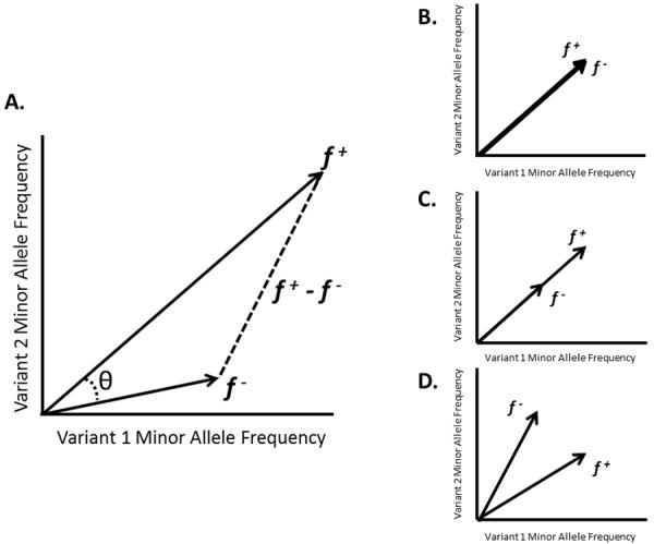
The set of graphs shows simplified scenarios for two rare variant sites in a case-control dataset and are designed to provide intuition into the geometric interpretation of rare variant tests.

A) The vectors f⁺ = (f₁⁺, f₂⁺) and f⁻ = (f₁⁻, f₂⁻) contain observed allele frequencies at two rare variant sites for cases and controls, respectively. ∥f⁺∥_p and ∥f⁻∥_p indicate the lengths of these frequency vectors with respect to the L_p norm, θ is the measure of the angle between f⁺ and, f⁻, and ∥f⁺ − f⁻∥_p is the distance between the endpoints of f⁺ and f⁻. The null hypothesis of no rare variant association (H₀: F⁺ = F⁻) can be tested using any of the three following null hypotheses related to the geometry of the frequency vectors: (i) ∥F⁺∥_p = ∥F⁻∥_p, the lengths of the vectors are equal, (ii) θ = 0, the angle between the vectors is zero, or (iii) ∥F⁺ − F⁻∥_p = 0, the distance between the endpoints of the vectors is zero. We refer to tests of the three geometric null hypotheses as, respectively, length, angle and joint tests. In the pictured scenario, the minor allele frequency is higher in cases for each variant (f₁⁺ > f₁⁻ and f₂⁺ > f₂⁻), indicating both as potential risk variants.

B) Under the null case of no association (F = F⁻) each of the geometric null hypotheses hold: (i) ∥F⁺∥_p = ∥F⁻∥_p, (ii) θ = 0, and (iii) ∥F⁺ − F⁻∥_p = 0.

C) Both variants are causative with the case vector being a scalar multiple of the control vector (F⁺ = cF⁻). This occurs if the case frequency and control frequency are the same across all variant sites. The result is that ∥F⁺∥_p ≠ ∥F⁻∥_p and ∥F⁺ − F⁻∥_p ≠ 0, but the null hypothesis of θ = 0 still holds. This scenario highlights the reason that angle tests are not powerful strategies and underscores why none have been proposed.

D) The scenario in which one rare variant is causative (f₁⁺ > f₁⁻) and the other is protective (f₂⁻ > f₂⁺). In this case, it is possible that ∥F⁺∥_p = ∥F⁻∥_p so that the signals from the two variants effectively cancel each other out, explaining reduced performance for length tests in the presence of a mix of risk and protective variants. Alternatively, ∥F⁺ − F⁻∥_p ≠ 0 and joint tests remain powerful.

In the following sections, we show that many rare variant tests of the null hypothesis H₀: F⁺ = F⁻ can be classified according to which geometric null hypothesis (eqs. 3, 4 or 6) is being tested (see Table 1).

Table 1.

Classifying existing rare variant tests using the geometric framework

	Length	Joint
Published Examples	CAST [Morgenthaler and Thilly, 2007]	CMC [Li and Leal, 2008]1
	CMC [Li and Leal, 2008]1	C-alpha [Neale et al., 2011]
	WS [Madsen and Browning, 2009]	SKAT [Wu et al., 2011]
	PR [Morris and Zeggini, 2010]	SSU [Basu and Pan, 2011]
	CMAT [Zawistowski et al., 2010]	GFRV [Lin and Tang, 2011]
	aSUM [Han and Pan, 2010]	AT [Pan and Shen, 2011]
	Variable Threshold[Price et al., 2010]	PRVT [Ionita-Laza et al., 2011]
	ORWSS [Feng et al., 2011]
	PWST [Zhang et al., 2011]
	RWAS[Sul et al., 2011]
	WHaIT [Li et al., 2011]
	WSCS [Dai et al., 2012]

¹CMC is a length test when all variants are below an arbitrarily defined MAF threshold; when some variants are above the threshold it acts as a combined length/joint test. See Appendices 1 and 2 for details.

A. Length Tests

We refer to rare variant tests of the null hypothesis H_0,Length: ∥F⁺∥_p = ∥F⁻∥_p as length tests. Here we show two examples of published statistics that are length tests. The cumulative minor allele test [CMAT; Zawistowski et al. 2010] compares the total number of minor and major alleles in cases and controls across rare, functional variants within the same gene. Using our notation, the test statistic for CMAT is ${\Sigma }_{\mathit{CMAT}}=\frac{N}{2N^{+}{N}^{-}m}\frac{c^{+}(2N^{-}-c^{-})-c^{-}(2N^{+}-c^{+})}{(c^{+}+c^{-})(2N^{-}-c^{-}+2N^{+}-c^{+})}$, where $c^{+}={\sum }_{i=1}^m{c}_j^{+}$, which can be simplified to Σ_CMAT = k(∥f⁺∥₁ − ∥f⁻∥₁), where k is a function of N⁺, N⁻, m and c = c⁺ + c⁻. The CMAT statistic is significant (as determined by permutation) when Σ_CMAT, and therefore ∥f⁺∥₁ − ∥f⁻∥₁, becomes large.

Proportion regression [PR; Morris and Zeggini, 2010] uses a logistic regression framework to test for a rare variant association. Specifically, PR uses the model $\mathrm{logit}\left({\pi }_i\right)=\alpha X_i+\beta \frac{r_i}{m}$where X_i is a vector of p covariate values for the i^th individual, α is the vector of marginal effects of the p covariates on the disease phenotype and $r_i={\sum }_{j=1}^m{c}_{ij}$ is the total number of rare alleles possessed by the i^th individual across the m variants. The score statistic $S={(y-{\widehat{\pi }}_0)}^{\prime }G{G}^{\prime }(y-{\widehat{\pi }}_0)$ is used to test H₀: β = 0, were y is a length N vector (N=total number of individuals in the study) of 0s and 1s, where 1=the individuals is a case, 0 otherwise, ${\widehat{\pi }}_0$ is a vector of predicted disease probabilities estimated under the null logistic model, and G is a vector containing r_i/m for each of the N individuals in the study. Under the null hypothesis of no association (<eq. 1>), S is distributed as a one degree of freedom chi-squared random variable. For simplicity, consider the case of no covariates and an equal number of cases and controls, which yields ${\widehat{\pi }}_0=\frac{1}{2}$ for all individuals. Then the PR score statistic can be written in terms of the vector length as follows

$$\begin{array}{c}\hfill S={(y-{\widehat{\pi }}_0)}^{\prime }{\mathit{GG}}^{\prime }(y-{\widehat{\pi }}_0)\propto 4{(y-{\widehat{\pi }}_0)}^{\prime }{\mathit{GG}}^{\prime }(y-{\widehat{\pi }}_0)\hfill \\ \hfill ={(2y-1)}^{\prime }{\mathit{GG}}^{\prime }(2y-1)\hfill \\ \hfill ={(G^{\prime }y-G^{\prime }(1-y\left)\right)}^{\prime }(G^{\prime }y-G^{\prime }(1-y\left)\right)\hfill \\ \hfill =\frac{N}{m^2}{({\parallel f^{+}\parallel }_1-{\parallel f^{-}\parallel }_1)}^2\hfill \end{array}$$

The null hypothesis H₀: β = 0 will be rejected for large S, which occurs when ∥f⁺∥₁ ≠ ∥f⁻∥₁.

We identified a total of twelve recently proposed rare variant tests as length tests based on the fact that significance of the test statistics was equivalent to testing ∥f⁺∥_p ≠ ∥f⁻∥_p (Appendix 1). Many length tests have been referred to in the literature as “burden” tests or “collapsing” tests [e.g., Dering et al. 2011]. In general, length tests measure how rare an individual is based on some index of the individual's cumulative rare allele profile across all variants in the set. This can be viewed as measuring the overall disease “burden” or “collapsing” all variants in the set. The aggregate level of burden within the cases is then compared to the aggregate burden in the controls to test for association.

B. Angle Tests

Tests of the null hypothesis H_0,Angle: θ = 0 are referred to as angle tests. To the best of our knowledge, no rare variant tests of this specific null hypothesis have been proposed. This is not necessarily a surprising observation because, as shown in Figure 1, if the case allele frequency vector, F⁺, is a scalar multiple of the control allele frequency vector, F⁻, as is the case when there is a consistent level of increased risk (the scalar multiple) across the set of variants, there will be no angle between the two vectors.

C. Joint Tests

We refer to rare variant tests of the null hypothesis H_0,Joint: ∥F⁺ − F⁻∥_p = 0 as joint tests since they jointly consider both the lengths and angles of the observed frequency vectors f⁺ and f⁻. A common example of a joint test is the Sequence Kernel Association Tests [SKAT, Wu et al. 2011]. Using a scaled version of SKAT with a linear unweighted kernel, we see that the test statistic is ${(y-{\widehat{\pi }}_{0}1)}^{\prime }A{A}^{\prime }(y-{\widehat{\pi }}_{0}1)\propto {\left(\frac{N}{\left(N^{+}\right)\left(N^{-}\right)}\right)}^2{(y-{\widehat{\pi }}_{0}1)}^{\prime }A{A}^{\prime }(y-{\widehat{\pi }}_{0}1)$ where A is an N × m genotype matrix containing the rare allele count of each individual at each site, y is an Nx1 vector indicating disease status (1 or 0) and ${\widehat{\pi }}_0$ = the fraction of cases in the sample. We note that ${\left(\frac{N}{\left(N^{+}\right)\left(N^{-}\right)}\right)}^2{(y-{\widehat{\pi }}_{0}1)}^{\prime }A{A}^{\prime }(y-{\widehat{\pi }}_{0}1)=$ ${\left(\frac{1}{N^{+}}y-\frac{1}{N^{-}}(1-y)\right)}^{\prime }A{A}^{\prime }\left(\frac{1}{N^{+}}y-\frac{1}{N^{-}}(1-y)\right)={(f^{+}-f^{-})}^{\prime }(f^{+}-f^{-})={\parallel f^{+}-f^{-}\parallel }_2^2$. Using similar rationale we classified six additional rare variant tests (Appendix 2). Appendix 2 also illustrates how SKAT can be considered as a joint test for many, but not all, kernel choices.

Unlike length tests, joint tests do not “collapse” or measure the overall individual disease burden in cases as compared to controls. Instead joint tests, by evaluating the length of the difference between the case and control vectors, consider differences in case-control allele frequency on a variant-by-variant basis, and then combine the variant-by-variant differences to obtain a statistic.

D. Novel tests suggested by the geometric framework

In addition to providing clarity on existing tests of association, the geometric framework also suggests alternative rare variant tests of association. In the following two sections we describe two alternative, generalized classes of rare variant tests of association that are direct implications of the geometric framework.

Alternative choice of norm

As shown in the previous sections many length tests use p=1, while most joint tests use p=2. While these choices are natural due to asymptotic theory of resulting test statistics and typical conceptualizations of geometric spaces, the geometric framework suggests that the choice of norm, p, in ∥x∥_p does not necessarily need to take values of 1 or 2. In particular, we can select any positive value for p, including infinity, ∞, where we define ∥x∥_∞ = arg max_i (x_i). Thus, we define the following generalized length (L_p) and joint (J_p) test statistics, with arbitrary choice of norm, p, as L_p = ∥f⁺∥_p − ∥f⁻∥_p and J_p = ∥f⁺ − f⁺∥_p. Appendix 3 provides an overview of how to modify L_p and J_p to handle covariates. Statistical significance is assessed via disease permutation. Note that L₁ is approximately equivalent to CMAT and J₂ is approximately equivalent to SKAT.

Weighted length-angle test

Another way the geometric framework can be used to generate new rare variant tests is by recognizing that length and angle tests represent two “extremes” in rare variant testing strategies. As noted earlier joint tests of the form ∥f⁺ − f⁻∥_p weight the “length” and “angle” portions of the test statistic approximately equally. This is a reasonable, though not necessary, choice. We define the following generalized joint test statistic, W, which gives the ability to increase or decrease the length or angle portion of the test by modifying w₁, as well as giving control over the choice of norm used through choice of p and q.

$$W(p,q,w_1)=w_1{({\parallel f^{+}\parallel }_p-{\parallel f^{-}\parallel }_p)}^2+(w_1-1)\cdot 2\cdot {\parallel f^{+}\parallel }_q\cdot {\parallel f^{-}\parallel }_q\cdot (1-\cos (\theta \left)\right)$$

Again, statistical significance is assessed via disease permutation. Appendix 3 provides a covariate adjusted version of W.

II. Simulation

We use two main simulation studies to validate select findings from our analysis. In the first simulation study we simulate 1500 cases and 1500 controls according to the following disease architecture. There are two rare variants in the set, each with a minor allele frequency of 1% in the controls in the populations from which the samples are selected. The choice of two variants was made to optimally illustrate the behavior of length and joint tests. As we will demonstrate later (Results), results easily generalize to any number of variants, m. Variant one has a fixed relative risk of 1.25, and we change the relative risk of variant two to take values of 0.2, 0.4, 0.6, 0.8, 1.0, 1.2, 1.4, 1.6, 1.8, 2.0, 2.5 and 3.0, for a total of 12 separate settings. At each setting we simulated 1000 sets of data. Empirical power estimates are calculated as the percentage of the 1000 simulated sets yielding a p-value less than 0.05. Three length tests (CMC, CMAT and PR) and two joint tests (SKAT (linear kernel), and C-alpha) were applied to the simulated data. Significance was determined by asymptotic distributions or 1000 permutations, depending upon the availability of an asymptotic distribution for the test. A smaller follow-up study considered a select set of these relative risks (0.2, 0.6, 1.0, 1.4 and 2.0) and applied a weighted length/angle test (described later; Results, C. Examples of further implications of the geometric framework)

In the second simulation study, we simulated 1000 cases and 1000 controls, according to the following disease model. We simulated eight causal variants: two with a minor allele frequency of 1%, and six with a minor allele frequency of 0.1% in the populations from which the samples are selected. All eight causal variants have a relative risk of 2.0. We then added increasing numbers of non-causal variants (in sets of 8, two at 1%/six at 0.1%). Ultimately, we considered 10 different simulation settings representing 0, 8, 16, 24, 32, 40, 48, 56, 64 and 72 non-causal variants in the set with the eight causal variants. Similar to the first simulation, we simulated 1000 sets of data at each setting to estimate empirical power. We considered four length test statistics, (∥f⁺∥_p − ∥f⁻∥_p)², with p=1,2,4 or ∞, and four different joint test statistics, ∥f⁺ − f⁻∥_p with p=1,2,4 or ∞, and where ∥x∥_∞ = max (|x_i|). Significance of these eight test statistics was assessed using 1000 permutations of case-control status.

Results

We have classified the majority of rare variant tests into one of two types: length or joint tests. In the following sections, we (a) present simulation results illustrating how the behavior of length and joint tests follows patterns suggested by the geometric framework (b) provided a detailed analysis of test behavior in light of genetic architecture and (c) demonstrate two specific ways that the geometric framework can be used to suggest modifications to existing rare variant tests of association.

A. Simulation results

Figure 1 and the overview of the geometric framework in the Methods section suggested that length tests focus solely on testing the null hypothesis that there is no difference in the lengths of the two allele frequency vectors, namely ∥F⁺∥_p = ∥F⁻∥_p, while joint tests focus on testing the null hypothesis that the length of the difference between the two allele frequency vectors, ∥F⁺ − F⁻∥_p is zero. We used simulation to confirm that the behavior of these values directly corresponds to the power of both length and joint tests (Figure 2).

Figure 2. Power of length and joint tests corresponds to the behavior predicted by geometric framework.

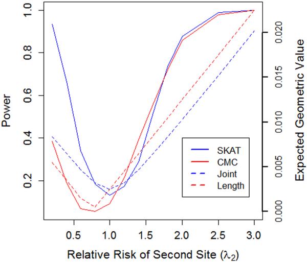
This graph illustrates the power of length and joint tests in relation to the expected value of the difference in lengths or length of difference of F⁺ and F⁻. In particular we consider the simplified scenario of a gene containing two rare variants, both with an allele frequency of 1%. The sample consists of 1500 cases and 1500 controls. The relative risk at the first variant site (λ₁) is fixed at 1.25, while the relative risk at the second site (λ₂) varies along the x-axis.

We plot the power of power of a length test (CMC) alongside the expected value of | ∥f⁺∥₂ − ∥f⁻∥₂|. The expected value of the length test statistic will be minimized (taking a value of zero) when the relative risk at site two is 0.75. As the relative risk at site two (λ₂) moves away from the value 0.75, the expected value of the length test statistic increases linearly. A similar pattern of behavior is observed for other length tests (e.g., CMAT and PR) though not shown here. We also plot the expected value of ∥f⁺ − f⁻∥₂ along with the power of a joint test (SKAT) Unlike length tests, joint tests attain their minimum value when λ₂=1, with the value of the expected value of both statistics increasing symmetrically as λ₂ moves away from 1. A similar pattern of behavior is observed for other joint tests (e.g., C-alpha), though not shown here.

B. Analytic insights into test behavior

Having provided an overview of the geometric framework and suggested intuition behind the behavior of different classes (Figure 1), as well as simulation results confirming this intuition (Figure 2), in the following sections we will explicitly demonstrate how genetic architecture affects the behavior of length, angle and joint tests. In particular we will explore how the three types of tests behave in relationship to three components of the genetic architecture of disease: (1) The relative risk of disease λ = (λ₁, λ₂, …, λ_m) where ${\lambda }_j\approx F_j^{+}∕F_j^{-}$, (2) the number of variants, m, in the gene and (3) the population minor allele frequencies at the m variant sites, F.

1. Changes in the relative risk distribution

For low prevalence diseases, $F_j^{-}\approx F_j$, and $F_j^{+}\approx {\lambda }_j{F}_j$, where λ_j is the relative risk of site j, and so λ_j>1 denotes a site where the rare allele increases disease risk, λ_j<1 denotes a site which reduces disease risk and λ_j=1 denotes a site that does not impact disease risk. We will use the terms risk, protective and non-causal site to denote these three cases, respectively.

Length tests

Length tests typically evaluate the difference between ∥f⁺∥_p and ∥f⁻∥_p which is equivalent to comparing ${\left({\sum }_{j=1}^m{\mid {\widehat{\lambda }}_j{f}_j\mid }^p\right)}^{\frac{1}{p}}\text{to}{\left({\sum }_{j=1}^m{\mid f_j\mid }^p\right)}^{\frac{1}{p}}$ where ${\widehat{\lambda }}_j$ is the MLE of λ_j. If F⁺ = F⁻, then, λ = (λ₁, λ₂, …, λ_m) = (1,1, …, 1) = 1, and so,

$${\left(\sum _{j=1}^m{\mid {\lambda }_j{F}_j\mid }^p\right)}^{\frac{1}{p}}={\left(\sum _{j=1}^m{\mid F_j\mid }^p\right)}^{\frac{1}{p}}$$ (eq. 8)

The limitation of length tests described earlier is demonstrated explicitly here, since λ = 1 is not a necessary condition for <eq. 8> to be true. In fact, there are an infinite number of values of λ which, for any given F, make <eq. 8> true, since <eq. 8> is an underdetermined equation (i.e. <eq. 8> is a single equation with m unknowns, namely λ₁, λ₂, …, λ_m for m>1). For example, consider the case where F_j = k for all j, and p=1. Then for any λ where ${\sum }_{j=1}^m{\lambda }_j=m$, <eq. 8> will be approximately true. In particular, if m=2, λ₁=1.25 and λ₂=0.75, then ${\sum }_{j=1}^m{\lambda }_j=2$ and, so, <eq. 8> is true. his example demonstrates that, within a gene with multiple variants at similar MAF, there will be little difference in ∥f⁺∥_p and ∥f⁻∥_p if the relative risks cancel out because some variants are risk and other variants are protective. Figure 2 illustrated this result.

Generally, a robust rare variant test of association will have the characteristic that the value of its test statistic will move farther from the null hypothesis value as |λ_j − 1| increases. However, for length tests the behavior of ∥f⁺∥_p − ∥f⁻∥_p as |λ_j − 1| increases is variable. In situations where all variants are risk (λ_j > 1 for all j) or all variants are protective (λ_j < 1 for all j) the difference in the lengths of ∥f⁺∥_p and ∥f⁻∥_p will increase as |λ_j − 1| increases. However, in cases where there is a mix of protective and risk variants (some λ_j are >1 and others are <1), the behavior of ∥f⁺∥_p − ∥f⁻∥_p may or may not increase. In particular, if ∥f⁺∥_p > ∥f⁻∥_p then increasing any λ_j will increase the difference in lengths of ∥f⁺∥_p and ∥f⁻∥_p, whereas if ∥f⁺∥_p < ∥f⁻∥_p decreasing any λ_j will increase the difference in lengths of ∥f⁺∥_p and ∥f⁻∥_p. Thus, length tests demonstrate a lack of robustness in the presence of mixes of risk and protective variants.

Joint tests

While length tests illustrate a lack of robustness in the presence of mixes of risk and protective variants, joint tests, in testing ∥F⁺ − F⁻∥_p = 0 do not have this same limitation. In general, $0={\parallel f^{+}-F^{-}\parallel }_p={\left({\sum }_{j=1}^m{\mid {\lambda }_j{F}_j-F_j\mid }^p\right)}^{1∕p}={\left({\sum }_{j=1}^m{F_j}^p{\mid {\lambda }_j-1\mid }^p\right)}^{1∕p}$, which is true if and only if,

$${\mid {\lambda }_j-1\mid }^p={\mid k_j\mid }^p=0\text{for all}j=1,\dots ,m$$ (eq. 9)

where λ_j = 1 + k_j, and k_j can be interpreted as the “risk deviation.”. <Eq. 9> is only true if and only if λ_j = 1 for all j, alternatively k_j = 0 for all j, which is true if and only if F⁺ = F⁻. Thus, a joint test which considers ∥f⁺ − f⁻∥_p equals 0 (the null hypothesis value) exactly when the null hypothesis is true. Alternatively, joint tests can be interpreted as finding the length of the allele frequency weighted risk deviations since ∥F⁺ − F⁻∥_p = ∥Fk∥_p. Implicitly, joint tests, unlike length tests, do not allow risk deviations to cancel out. Furthermore, it is clear from <eq.9> that joint tests are robust to mixes of risk and protective variants since the value of ∥F⁺ − F⁻∥_p will increase as |λ_j − 1| increases. Figure 2 provides an example of this behavior.

Angle tests

Our results thus far suggest that handling mixes of protective/risk variants may be problematic for length tests, while joint tests more appropriately handle mixes of protective/risk variants. Thus, since joint tests are testing a combined hypothesis which considers both length and angle differences in the vectors (see Methods), this suggests that angle tests might be robust to mixes of protective and risk variants.

To test this claim, note that when the null hypothesis (F⁺ = F⁻) is true, there is no angle between the two vectors (θ = 0). When θ = 0, then F⁺ · F⁻ = ∥F⁺∥₂ · ∥F⁻∥₂, or alternately, ${\sum }_{j=1}^m{\lambda }_j{F_j}^2=\sqrt{{\sum }_{j=1}^m{\left({\lambda }_j{F}_j\right)}^2}\sqrt{{\sum }_{j=1}^m{\left(F_j\right)}^2}$. But, we note that if λ = l (l > 0; a constant value for all λ_j) then

$$\sqrt{\sum _{j=1}^m{\left({\lambda }_j{F}_j\right)}^2}\sqrt{\sum _{j=1}^m{\left(F_j\right)}^2}=\sqrt{\sum _{i=1}^m\sum _{j=1}^m{\left({\lambda }_i{F}_i\right)}^2{\left(F_j\right)}^2}=l\sqrt{\sum _{i=1}^m\sum _{j=1}^m{\left(F_i\right)}^2{\left(F_j\right)}^2}=l\sqrt{{\left(\sum _{j=1}^m{F_j}^2\right)}^2}=l\left(\sum _{j=1}^m{F_j}^2\right).$$

Thus, there is no angle between vectors F⁺ and F⁻ whenever λ = l, not only when the null hypothesis is true (l=1). In general, larger angles will occur as the values of λ_j become increasingly different (spread out), as will occur when there are mixes of risk and protective variants. However, when values of λ_j are not that different, there will be little difference in the angle between the two vectors, even if the values of λ_j are different than 1. Thus, importantly, sets of variants showing consistent levels of risk or consistent levels of protection will yield minimal angles between the case and control allele frequency vectors. For example, if all variants in the set had a relative risk of 2 (λ = 2) there would be no angle between the two vectors; refer also to Figure 1c. Hence, angle tests, like length, show lack of robustness to a plausible scenario for the values of λ.

2. Changes in minor allele frequency

In the previous section, we described how changes to the relative risk distribution impact length, angle and joint tests. With these results in mind, we now turn our attention to how changes in the minor allele frequency vector, F impact the general behavior of length and joint tests.

Increasing the minor allele frequency, F_j, at a particular site j, will have different effects on the difference in lengths of the case and control allele frequency vectors, ∥f⁺∥_p − ∥f⁻∥_p, depending upon the value of λ_j and the starting value of ∥f⁺∥_p − ∥f⁻∥_p. In particular, increasing F_j for a risk variant (λ_j > 1) will decrease the value of ∥f⁺∥_p − ∥f⁻∥_p if ∥f⁺∥_p > 0 before the change. Increasing F_j for a protective variant (λ_j > 1) will decrease the difference in lengths, and when λ_j = 1, changing F_j does not change the difference in lengths. In contrast, for joint tests, the impact of minor allele frequency, F, on ∥f⁺ − f⁻∥_p is straightforward. Simply stated, since ${\parallel f^{+}-f^{-}\parallel }_p={\left({\sum }_{j=1}^m{F_j}^p{\mid {\lambda }_j-1\mid }^p\right)}^{1∕p}$, increases to the minor allele frequencies F_j will always increase the value of ∥f⁺ − f⁻∥_p regardless of λ.

3. Number of variants

For length tests, the impact of increasing the number of variants, m, in the set is straightforward. Simply stated, if the length of the case vector (∥f⁺∥_p) is greater than the length of the control vector (∥f⁻∥_p) before adding the additional variant, then if the additional variant has f_j⁺ > f_j⁻, the difference in lengths will increase whereas if f_j⁺ < f_j⁻ the difference in lengths will decrease. The addition of non-causal variants will, on average, increase both the case and control vectors a similar amount and, thus, have no impact on the difference in lengths. However, for joint tests, the value of ${\parallel f^{+}-f^{-}\parallel }_p={\left({\sum }_{j=1}^m{f_j}^p{\mid {\lambda }_j-1\mid }^p\right)}^{1∕p}$ will increase with the addition of each causal variant (λ_j ≠ 1) and, on average, remain the same for non-causal variants (λ_j = 1) that are added to the set being tested.

C. Examples of further implications of the geometric framework

In the previous sections we have described how the geometric framework provides direct insight into the behavior of length and joint tests. The geometric framework also suggests alternative rare variant tests of association, with predictable behavior. Earlier, we proposed two generalized tests suggested by the geometric framework. In the following two sections we describe the behavior of these tests on simulated data.

1. The impact of the choice of norm, p

Earlier, we proposed generalized length and joint test statistics, L_p and J_p, which allowed researchers to select any positive value, p>0 or ∞, for p. We now explore the behavior of these test statistics as a function of the choice of norm, p.

In most realistic situations, a fraction of the m variants will have λ_j = 1 since it is difficult to identify, a priori, which of the variants in a set are causal (λ_j ≠ 1) Thus, in the observed sample, many of the estimated relative risks will be different from 1 only by chance—not reflecting a population relative risk different than 1. Intuitively, by increasing p, we are able to mitigate the effect of non-causal sites on the test statistic, by, in essence, up-weighting larger observed effects. Ultimately, this translates into a mitigation of decreased power from the addition of non-causal sites, as seen in Figures 3a and 3b for L_p and J_p, respectively. Importantly, we see a complete reversal in the ordering of most powerful tests as we move from 0 to 72 non-causal sites for the length test, and a near complete reversal for the joint test.

Figure 3. Power of length and joint tests corresponds to the behavior predicted by geometric framework.

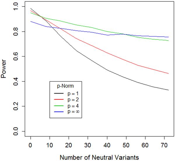
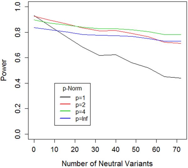
The two graphs illustrate the power of length (L_p = ∥f⁺∥_p − ∥f⁻∥_p)and joint tests (J_p = ∥f⁺ − f⁻∥_p) with different norms (p=1, 2, 4 and ∞). In each case the test statistic is computed and significance is assessed via permutation of case-control status. We consider a scenario where a gene contains eight causal risk variants, all with a relative risk of 2.0. Two of the risk variants have MAF=1%, the other six have MAF=0.1%. We simulated a sample of 1000 cases and 1000 controls for this setting. We then considered 9 additional settings where we added 8, 16, 24, 32, 40, 48, 56, 64 and 72 additional non-causal variants (relative risk=1), always maintaining 3:1 ratio of low MAF (0.1%) to high MAF (1%) variants in the set.

A) For L_p, as we move from no non-causal variants to 72 non-causal variants, the order of most powerful tests completely reverses, suggesting that higher norms are more optimal in situations with large numbers of non-causal variants.

B) For L_p, as we move from no non-causal variants to 72 non-causal variants, the order of most powerful tests nearly reverses, suggesting that, once again, higher norms are more optimal in situations with large numbers of non-causal variants.

The intuition in Figure 3 can be confirmed by looking more carefully at the formulation of the test statistics. For J_p, in all cases, increasing p, means that larger allele frequency weighted risk deviations, ${f_j}^p{\mid {\widehat{\lambda }}_j-1\mid }^p$, are counted proportionally more in $J_p={\parallel f^{+}-f^{-}\parallel }_p={\left({\sum }_{j=1}^m{f_j}^p{\mid {\widehat{\lambda }}_j-1\mid }^p\right)}^{1∕p}$. For L, a similar result also holds. Consider a case where the allele frequency at all variant sites is constant, f_j = f for all j. Then, $L_p={\parallel f^{+}\parallel }_p-{\parallel f^{-}\parallel }_p\approx {\left(f^p{\sum }_{j=1}^m{\mid {\widehat{\lambda }}_j\mid }^p\right)}^{\frac{1}{p}}-{\left({\mathit{mf}}^p\right)}^{\frac{1}{p}}=f{\left({\sum }_{j=1}^m{\mid {\widehat{\lambda }}_j\mid }^p\right)}^{\frac{1}{p}}-f{\left(m\right)}^{\frac{1}{p}}=f\left({\left({\sum }_{j=1}^m{\mid {\widehat{\lambda }}_j\mid }^p\right)}^{\frac{1}{p}}-{\left(m\right)}^{\frac{1}{p}}\right)$. Thus, if all ${\widehat{\lambda }}_j\rangle 1$, increasing p means that variants with larger estimated risk will be counted proportionally more when finding the difference in lengths. In situations where f is not constant, the same general result holds, but may be mitigated or exacerbated based on the allele frequencies of the non-causal and causal variants. Thus, higher choices of norms exhibit more robustness to the inclusion of neutral variants by upweighting larger effects and downweighting weaker effects observed in the sample data.

2. Fine-tuned combinations of length and joint tests

Earlier, we defined W(w₁, p, q) = w₁(∥f⁺∥_p − ∥f⁻∥_p)² + (w₁ − 1) · 2 · ∥f⁺∥_q · ∥f⁻∥_q · (1 − cos (θ)). Thus, W(w₁, p, q) gives more fine-tuned control over the contribution of length and angle differences to the test statistic. Most joint tests implicitly let w₁ = 0.5. Figure 4 illustrates that more powerful tests can be obtained for particular relative risks by modifying w₁.

Figure 4. Arbitrary combining of length and angle tests.

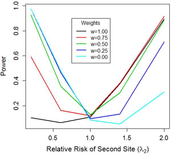
We conducted a simulation analysis and used W(W₁, p, q) with p=q=2, and let w₁ = 1 (length only), w₁ = 0.75, w₁ =0.5 (typical joint test), w₁ =0.25 and w₁0 (angle only test). Figure 4 illustrates the power of these five tests across different values of λ₂. Power curves are as predicted. In particular, the length only (w₁ =1) and angle only (w₁ =0) tests show the least robustness, while the (w₁ =0.5) test is quite robust. As expected, the (w₁ =0.75) weighted test outperforms the (w₁ =0.5) test when both variants are risk-inducing, while providing more power than the length only test when there is a mix of risk-inducing and protective variants. The reverse is true for the (w₁ =0.25) test.

Discussion

Observing all variation in large genetic datasets is fast becoming a reality due to high throughput sequencing technologies. However, an open question is how to best use these datasets in order to test for association between rare variants and phenotypes of interest. The current strategy is to simultaneously analyze multiple rare variants in the same gene in a single statistic, with at least 18 such methods having been proposed to date. While the underlying intuition for some tests provides a means for determining which are similar, in other cases it is less obvious how they are related. Here, we have derived a formal geometric framework that provides a rigorous method for comparing many existing rare variant tests. Further, we have identified strategies to increase statistical power both by adjusting features of existing tests and by combining existing tests with different properties.

When placed in context of this geometric framework, we find that the major distinguishing characteristic of rare variant tests is how they handle variants with opposing directions of effect. The geometric framework differentiates between tests that are robust to a mix of risk and protective variants (joint tests) and those that are most powerful when all causal variants have the same direction of effect (length tests). While this distinction was previously known to exist, we are now able to attribute the difference in performance to a theoretical difference in the underlying null hypotheses of the respective tests. By decomposing the compound null hypothesis of no phenotype association within a set of multiple rare variants into simple null hypotheses, it becomes clear that a “rare variant association” can be interpreted in different fashions. Namely, a rare variant association can be either a difference between cases and controls in the cumulative frequency of all rare alleles as assumed by the length tests, or a pattern of frequency differences for individual variants as assumed by the joint tests. Both definitions of rare variant association are entirely reasonable and there are likely to be traits and susceptibility genes that satisfy each definition.

We classified many existing rare variant tests according to the geometric framework, including the most common and cited methods; most could be categorized as either a length or a joint test. Thus, despite the number and seeming diversity of rare variant tests proposed to date, they are actually quite similar in philosophy. However, we did observe some tests which did not obviously fit the geometric framework; for example, Bayesian approaches [Quintana et al. 2011; Yi and Zhi 2011], extensions of single-marker methods [Li, Zhang and Yu 2010] and other approaches [Wu et al. 2011 with a non-additive kernel]. We do not view the existence of such methods as a limitation of the geometric framework, but rather a dramatic shift in methodology from what has largely been developed to date. If a test satisfies the definition of neither a length nor a joint test, it could benefit the field as it would introduce alternative interpretations of the rare variant problem and potentially improve our ability to discover rare variant associations.

The geometric framework provides several practical applications to rare variant analysis. With performance known to differ between tests, however subtly, investigators are likely to apply multiple gene-based tests to the same dataset. The geometric classification method can be a useful tool in planning an analysis that includes multiple tests on the same set of rare variants. The investigator can choose a set of tests that provide complementary pieces of information, for example ensuring both length and joint-style tests are applied. If some prior knowledge of the underlying genetic architecture is available, it can inform the set of tests that are likely to perform best. The geometric framework can also aid in the interpretation of the results from multiple rare variant tests. Given that we can predict which tests should produce similar p-values based on their classification (length versus joint), differences in significance can be attributed to additional factors such as variant weighting schemes, which in turn can be valuable for interpreting a significant association signal. For example, frequency-based weights that increase significance of a test may provide some information on the underlying frequency spectrum of causal variants. Furthermore, tests within each category are likely to perform similarly with respect to artifacts in the data such as genotyping errors [Powers et al. 2011; Mayer-Jochimsen et al. 2012] and population stratification [Zawistowski et al. 2012]. Thus, methodological research in these areas may not need to consider each of the many rare variant tests individually, but rather consider implications within each broad class of tests.

Our exploration of the effect of norms on test power also has implications for rare variant analysis designs. Combining multiple rare variants into a single test statistic leads to an inevitable signal to noise problem due to the inclusion of non-causal variants. In our analysis, we observed that the value of the norm used to compute distance between case and control frequency vectors in a rare variant statistic contributes to the robustness of that statistic to the inclusion of non-causal variants in the analysis. We showed that in some cases increasing the norm of the statistic can reduce power loss for inclusion of non-causal variants. However, only norms of p=1 and p=2 have been used to date, indicating that this is a relatively unexplored aspect of handling the signal to noise problem in rare variant testing.

This is noteworthy because the common current strategy for reducing the inclusion of non-causal variants is to combine only non-synonymous and nonsense coding variants within a gene since these are assumed to be most likely to be causal. This strategy ignores the potential deleterious effect of non-coding and synonymous variants, both of which have been shown in some cases to contribute to disease risk. In particular, the ENCODE database highlights the critical role that the non-coding portion of the genome plays in gene expression [ENCODE, 2012]. Efficiently incorporating non-coding variation into rare variant tests while controlling for non-causal variants may be a powerfully strategy for detecting novel associations. The increased-norm approach provides an alternative to the nonsynonymous-only approach of controlling power loss due to inclusion of non-causal variants with the advantage that it allows a more complete set of rare variation in the gene, particularly non-coding variants, to be investigated.

The categorization of tests based on assumptions of risk and protective variants helps to systematically explain some of the differences in performance between rare variant tests. However, there are likely several additional factors that can impact performance, most notably variant weighting strategies. Weighting rare variants based on some criteria of evidence for association is a common strategy to attempt to increase power and includes allele frequency-based weights, quantitative predictions of the damaging impact of a variant or a measure of conservation across species. Though we have not directly considered it here, the geometric framework can provide a context for evaluating the effect of various weighting strategies. The weighted variants can be viewed as transformations of the original genotype frequency vectors, and the merits of a weighting strategy could be determined by comparing the change in the original and transformed vectors. For example, if we considered weighting strategies for a length test, a set of weights would be beneficial if the weighted case and control vectors have a larger difference in normed length than did the original unweighted vectors.

The geometric framework presented here provides a rather unique perspective on the current field of rare variant association tests. In addition to improving our understanding of why certain tests perform as they do and which are methodologically most similar, we have also uncovered areas in which future modifications can be made to existing rare variant tests to improve power to detect associations.

References

- 1000 Genomes Project Consortium A map of human genome variation from population-scale sequencing. Nature. 2010;467:1061–1073. doi: 10.1038/nature09534. [DOI] [PMC free article] [PubMed] [Google Scholar]
- Asimit J, Zeggini E. Rare variant association analysis methods for complex traits. Annu Rev Genet. 2010;44:293–308. doi: 10.1146/annurev-genet-102209-163421. [DOI] [PubMed] [Google Scholar]
- Bansal V, Libiger O, Torkamani A, Schork NJ. Statistical analysis strategies for association studies involving rare variants. 2010;11:773–785. doi: 10.1038/nrg2867. [DOI] [PMC free article] [PubMed] [Google Scholar]
- Basu S, Pan W. Comparison of statistical tests for disease association with rare variants. Genet Epidemiol. 2011;35:606–619. doi: 10.1002/gepi.20609. [DOI] [PMC free article] [PubMed] [Google Scholar]
- Cooper GM, Shendure J. Needles in stacks of needs: finding disease causal variants in a wealth of genomic data. Nat Genet. 2011;12:628–640. doi: 10.1038/nrg3046. [DOI] [PubMed] [Google Scholar]
- Dai Y, Jiang R, Dong J. Weighted selective collapsing strategy for detecting rare and common variants in genetic association study. BMC Genet. 2012;13:7. doi: 10.1186/1471-2156-13-7. [DOI] [PMC free article] [PubMed] [Google Scholar]
- Dering C, Pugh E, Ziegler A. Statistical analysis of rare sequence variants: an overview of collapsing methods. Genet Epidemiol. 2011;35:S12–S17. doi: 10.1002/gepi.20643. [DOI] [PMC free article] [PubMed] [Google Scholar]
- The ENCODE Project Consortium An integrated encyclopedia of DNA elements in the human genome. Nature. 2012;489:57–74. doi: 10.1038/nature11247. [DOI] [PMC free article] [PubMed] [Google Scholar]
- Feng T, Elston RC, Zhu X. Detecting rare and common variants for complex traits: sibpair and odds ratio weighted sum statistics (SPWSS, ORWSS) Genet Epidemiol. 2011;35:398–409. doi: 10.1002/gepi.20588. [DOI] [PMC free article] [PubMed] [Google Scholar]
- Gibson G. Rare and common variants: twenty arguments. Nat Rev Genet. 2012;13:135–145. doi: 10.1038/nrg3118. [DOI] [PMC free article] [PubMed] [Google Scholar]
- Han F, Pan W. A data-adaptive sum test for disease association with multiple common or rare variants. Hum Hered. 2010;70:42–54. doi: 10.1159/000288704. [DOI] [PMC free article] [PubMed] [Google Scholar]
- Ionita-Laza I, Buxbaum JD, Laird NM, Lange C. A new testing strategy to identify rare variants with either risk or protective effect on disease. PLos Genet. 2011;7:e1001289. doi: 10.1371/journal.pgen.1001289. [DOI] [PMC free article] [PubMed] [Google Scholar]
- Ladouceur M, Dastani Z, Aulchenko YS, Greenwood CMT, Richards JB. The empirical power of rare variant association methods: results from sanger sequencing in 1998 individuals. PLoS Genet. 2012;8:e1002496. doi: 10.1371/journal.pgen.1002496. [DOI] [PMC free article] [PubMed] [Google Scholar]
- Li B, Leal SM. Methods for detecting associations with rare variants for common diseases: application to analysis of sequence data. Am J Hum Genet. 2008;83:311–321. doi: 10.1016/j.ajhg.2008.06.024. [DOI] [PMC free article] [PubMed] [Google Scholar]
- Li Y, Byrnes AE, Li M. To identify associations with rare variants, just WHaIT: weighted haplotype and imputation-based tests. Am J Hum Genet. 2011;87:728–735. doi: 10.1016/j.ajhg.2010.10.014. [DOI] [PMC free article] [PubMed] [Google Scholar]
- Lin D, Tang Z. A general framework for detecting disease associations with rare variants in sequencing studies. Am J Hum Genet. 2011;89:354–67. doi: 10.1016/j.ajhg.2011.07.015. [DOI] [PMC free article] [PubMed] [Google Scholar]
- Luedtke A, Powers S, Petersen A, Sitarik A, Bekmetjev A, Tintle NL. Evaluating methods for the analysis of rare variants in sequence data. BMC Proc. 2011;5:S119. doi: 10.1186/1753-6561-5-S9-S119. [DOI] [PMC free article] [PubMed] [Google Scholar]
- Li Q, Zhang H, Yu K. Approaches for evaluating rare polymorphisms in genetic association studies. Hum Hered. 2010;69:219–228. doi: 10.1159/000291927. [DOI] [PMC free article] [PubMed] [Google Scholar]
- Madsen BE, Browning SR. A groupwise association test for rare mutations using a weighted sum statistic. PLoS Genet. 2009;5:e1000384. doi: 10.1371/journal.pgen.1000384. [DOI] [PMC free article] [PubMed] [Google Scholar]
- Mayer-Jochimsen M, Fast S, Tintle NL. “Assessing the impact of differential genotyping errors on rare variant tests of association” In revision. PLoS One. 2012 doi: 10.1371/journal.pone.0056626. [DOI] [PMC free article] [PubMed] [Google Scholar]
- Morgenthaler S, Thilly WG. A strategy to discover genes that carry multiallelic or mono-allelic risk for common diseases: A cohort allelic sums test (CAST) Mutat Res Fund Mol Mech Mut. 2007;615:28–56. doi: 10.1016/j.mrfmmm.2006.09.003. [DOI] [PubMed] [Google Scholar]
- Morris AP, Zeggini E. An evaluation of statistical approaches to rare variant analysis in genetic association studies. Genet. Epidemiol. 2010;34:188–193. doi: 10.1002/gepi.20450. [DOI] [PMC free article] [PubMed] [Google Scholar]
- Neale BM, Rivas MA, Voight BF, Altshuler D, Devlin B, Orho-Melander M, Kathiresan S, Purcell SM, Roeder K, Daly MJ. Testing for an unusual distribution of rare variants. PLoS Genet. 2011;7:e1001322. doi: 10.1371/journal.pgen.1001322. [DOI] [PMC free article] [PubMed] [Google Scholar]
- Nelson MR, Wegmann D, Ehm MG, Kessner D, St. Jean P, Verzilli C, Shen J, Tang Z, Bacanu S, Fraser D, et al. An abundance of rare functional variants in 202 drug target genes sequenced in 14,002 people. Sci. To appear. 2012 doi: 10.1126/science.1217876. [DOI] [PMC free article] [PubMed] [Google Scholar]
- Pan W, Shen X. Adaptive tests for association analysis of rare variants. Genet Epidemiol. 2011;35:381–388. doi: 10.1002/gepi.20586. [DOI] [PMC free article] [PubMed] [Google Scholar]
- Powers S, Gopalakrishnan S, Tintle NL. Assessing the impact of non-differential genotyping errors on rare variant tests of association. Hum Hered. 2011;72:152–159. doi: 10.1159/000332222. [DOI] [PMC free article] [PubMed] [Google Scholar]
- Price AL, Kryukov GV, de Bakker PIW, Purcell SM, Staples J, Wei L, Sunyaev SR. Pooled association tests for rare variants in exon-resequencing studies. Am J Hum Genet. 2010;86:832–838. doi: 10.1016/j.ajhg.2010.04.005. [DOI] [PMC free article] [PubMed] [Google Scholar]
- Quintana MA, Berstein JL, Thomas DC, Conti DV. Incorporating model uncertainty in detecting rare variants: the Bayesian risk index. Genet Epidemiol. 2011;35:638–649. doi: 10.1002/gepi.20613. [DOI] [PMC free article] [PubMed] [Google Scholar]
- Rivas MA, Beaudoin M, Gardet A, Stevens C, Sharma Y, Zhang CK, Boucher G, Ripke S, Ellinghaus D, Burtt N, et al. Deep resequencing of GWAS loci identifies independent rare variants associated with inflammatory bowel disease. Nat Genet. 2011;43:1066–1075. doi: 10.1038/ng.952. [DOI] [PMC free article] [PubMed] [Google Scholar]
- Sul J, Han B, He D, Eskin E. An optimal weighted aggregated association test for identification of rare variants involved in common diseases. Genet. 2011;188:181–188. doi: 10.1534/genetics.110.125070. [DOI] [PMC free article] [PubMed] [Google Scholar]
- Sun YV, Sung YJ, Tintle NL, Ziegler A. Identification of genetic association of multiple rare variants using collapsing methods. Genet Epidemiol. 2011;35:S101–S106. doi: 10.1002/gepi.20658. [DOI] [PMC free article] [PubMed] [Google Scholar]
- Tennessen JA, Bigham AW, O'Connor TD, Fu W, Kenny EE, Gravel S, McGee S, Do R, Liu X, Jun G, et al. Evolution and functional impact of rare coding variation from deep sequencing of human exomes. Sci. To appear. 2012 doi: 10.1126/science.1219240. [DOI] [PMC free article] [PubMed] [Google Scholar]
- Tintle NL, Aschard H, Hu I, Nock N, Wang H, Pugh E. Inflated type I error rates when using aggregation methods to analyze rare variants in the 1000 genomes project exon sequencing data in unrelated individuals: summary results from group 7 at genetic analysis workshop 17. Genet Epidemiol. 2011;35:S56–S60. doi: 10.1002/gepi.20650. [DOI] [PMC free article] [PubMed] [Google Scholar]
- Torgerson DG, Capurso D, Mathias RA, Graves PE, Hernandez RD, Beaty TH, Bleecker ER, Raby BA, Meyers DA, Barnes KC, et al. Resequencing candidate genes implicates rare variants in asthma susceptibility. Am J Hum Genet. 2012;90:273–281. doi: 10.1016/j.ajhg.2012.01.008. [DOI] [PMC free article] [PubMed] [Google Scholar]
- Wu MC, Lee S, Cai T, Li Y, Boehnke M, Lin X. Rare-variant association testing for sequence data with the sequence kernel association test. Am J Hum Genet. 2011;89:82–93. doi: 10.1016/j.ajhg.2011.05.029. [DOI] [PMC free article] [PubMed] [Google Scholar]
- Yi N, Zhi D. Bayesian analysis of rare variants in genetic association studies. Genet Epidemiol. 2011;35:57–69. doi: 10.1002/gepi.20554. [DOI] [PMC free article] [PubMed] [Google Scholar]
- Zawistowski M, Gopalakrishnan S, Ding J, Li Y, Grimm S, Zollner S. Extending rare-variant testing strategies: analysis of noncoding sequence and imputed genotypes. Am J Hum Genet. 2010;87:604–617. doi: 10.1016/j.ajhg.2010.10.012. [DOI] [PMC free article] [PubMed] [Google Scholar]
- Zawistowski M, Reppell M, Wegmann D, St. Jean PL, Ehm MG, Nelson MR, Novembre J, Zollner S. Differential stratification in rare variant tests observed using an analytic model of joint site frequency spectra. 2012 Unpublished manuscript. [Google Scholar]
- Zhang Q, Irvin MR, Arnett DK, Province MA, Borecki I. A data-driven method for identifying rare variants with heterogeneous trait effects. Genet Epidemiol. 2011;35:679–685. doi: 10.1002/gepi.20618. [DOI] [PMC free article] [PubMed] [Google Scholar]
Associated Data
This section collects any data citations, data availability statements, or supplementary materials included in this article.