Phase separation explains a new class of self-organized spatial patterns in ecological systems

Abstract

The origin of regular spatial patterns in ecological systems has long fascinated researchers. Turing’s activator–inhibitor principle is considered the central paradigm to explain such patterns. According to this principle, local activation combined with long-range inhibition of growth and survival is an essential prerequisite for pattern formation. Here, we show that the physical principle of phase separation, solely based on density-dependent movement by organisms, represents an alternative class of self-organized pattern formation in ecology. Using experiments with self-organizing mussel beds, we derive an empirical relation between the speed of animal movement and local animal density. By incorporating this relation in a partial differential equation, we demonstrate that this model corresponds mathematically to the well-known Cahn–Hilliard equation for phase separation in physics. Finally, we show that the predicted patterns match those found both in field observations and in our experiments. Our results reveal a principle for ecological self-organization, where phase separation rather than activation and inhibition processes drives spatial pattern formation.

The activator–inhibitor principle, originally conceived by Turing in 1952 (1), provides a potential theoretical mechanism for the occurrence of regular patterns in biology (2–6) and chemistry (7–9), although experimental evidence in particular for biological systems has remained scarce (3, 4, 10). In the past decades, this principle has been applied to a wide range of ecological systems, including arid bush lands (11–15), mussel beds (16, 17), and boreal peat lands (18, 19). The principle, in which a local positive activating feedback interacts with large-scale inhibitory feedback to generate spatial differentiation in growth, birth, mortality, respiration, or decay, explains the spontaneous emergence of regular spatial patterns in ecosystems even under near-homogeneous starting conditions. Physical theory offers an alternative mechanism for pattern formation, proposed by Cahn and Hilliard in 1958 (20). They identified that density-dependent rates of dispersal can lead to separation of a mixed fluid into two phases that are separated in distinct spatial regions, subsequently leading to pattern formation. The principle of density-dependent dispersal, switching between dispersion and aggregation as local density increases, has become a central mathematical explanation for phase separation in many fields (21) such as multiphase fluid flow (22), mineral exsolution and growth (23), and biological applications (24–28). Although aggregation due to individual motion is a commonly observed phenomenon within ecology, application of the principles of phase separation to explain pattern formation in ecological systems is absent both in terms of theory and experiments (25, 26).

Here, we apply the concept of phase separation to the formation of spatial patterns in the distribution of aggregating mussels. On intertidal flats, establishing mussel beds exhibit spatial self-organization by forming a pattern of regularly spaced clumps. By so doing, they balance optimal protection against predation with optimal access to food, as demonstrated in a field experiment (29). This self-organization process has been attributed to the dependence of the speed of movement on local mussel density (29). Mussels move at high speed when they occur in low density and decrease their speed of movement once they are included in small clusters. However, when occurring in large and dense clusters, they tend to move faster again, due to food shortage. Mussel pattern formation is a fast process, giving rise to stable patterning within the course of a few hours, and clearly is independent from birth or death processes (Fig. 1 A and B). Although mussel pattern formation at centimeter scale was successfully reproduced by an empirical individual-based model (29), to date no satisfactory continuous model has been reported that can identify the underlying principle in a general theoretical context.

Fig. 1.

Pattern formation in mussels and statistical properties of the density-dependent movement of mussels under experimental laboratory conditions. (A and B) Mussels that were laid out evenly under controlled conditions on a homogeneous substrate developed spatial patterns similar to “labyrinth-like” after 24 h (images represent a surface of 60 cm × 80 cm). (C) Relation between movement speed and density within a series of mussels clusters (mussel density is rescaled, where 128 equals to 1). The blue line describes the rescaled second-order polynomial fit with Eq. 1. The red line depicts the effective diffusion of mussels as a function of the local densities according to the diffusion-drift theory. The open circles show the original experiment data, and the solid squares represent the average speed of each group. (D) The numerical simulation of Eq. 4 implemented with parameters , , and , simulating the development of spatial patterns from a near-uniform initial state.

In this paper, we present the derivation and analysis of a partial differential equation model based on an empirical description of density-dependent movement in mussels, and demonstrate that it is mathematically equivalent to the original model of phase separation by Cahn and Hilliard (20). We then compare the predictions of this model with observations from real mussel beds and experiments with mussel pattern formation in the laboratory.

Results

Model Description.

Mussel speed of movement was observed to initially decrease with increasing mussel density, but to increase when the density exceeded that typically observed in nature (Fig. 1C). The movement speed data were fitted to the following equation:

with and (Fig. 1C, blue line). A linear model proved not significant (P = 0.449). The quadratic model was overall significant (P < 0.001), where the coefficient for the second-order term was highly significant (t = 5.717, P < 0.0001), and the Akaike information criterion test showed that the quadratic model was highly preferable over the linear one (see Table S1 for details). Note that we used a quadratic equation not because it provides the most optimal fit, but because it is the most simple polynomial function.

Based on this formulation, we now derive an equation for the changes in local density M of a population of mussels, in a 2D space. As the model describes pattern formation at timescales shorter than 24 h, growth and mortality (as factors affecting local mussel density) can be ignored. Local fluxes of mussels at any specific location can therefore be described by the generic conservation equation:

Here, is the net flux of mussels, and 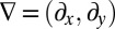is the gradient in two dimensions.

To derive the net flux J, we assume that mussel movement can be described as a random, step-wise walk with a step size V that is a function of mussel density, and a random, uncorrelated reorientation. In the case of density-dependent movement, the net flux arising from the local gradient in mussel density can be expressed as follows (SI Text):

where is the turning rate, following Schnitzer (30) (equation 4.14 of ref. 30). The “drift” term accounts for the effect of spatial variation in local mussel density on the spatial flux of mussels. This term does not appear in the case of density-independent movement, but its contribution is crucial when up-scaling the density-dependent movement of individuals to the population level.

Following earlier treatments of biological diffusion as a result of individual movement (2), we complement this local diffusion term with a term that accounts for the long-distance movement by including nonlocal diffusion as with nonlocal diffusion coefficient . The nonlocal diffusion process has a relatively low intensity, and hence parameter is much smaller in magnitude than the local movement coefficient in Eq. 3. We can now gather both fluxes into the total net flux rate in Eq. 2, , to define the general rescaled conservation equation as follows (SI Text):

Here, , where is a rescaled speed. is a rescaled diffusion coefficient that describes the average mussel movement, and is the rescaled nonlocal diffusion coefficient. Rescaling at the basis of Eq. 4 is given by the following relations: with , , , and . Here, captures the depression of diffusion at intermediate densities in a single parameter. In this model, spatial patterns develop once the inequalities and are satisfied, leading to a negative effective diffusion (aggregation) at intermediate mussel densities. Thus, if mussel movement is significantly depressed at intermediate density, then effective diffusion becomes negative, mussels aggregate, and patterns emerge. If the depression of mussel movement speed at intermediate mussel density is weak, then remains positive, and no aggregation occurs at intermediate biomass (Fig. S1). Under these conditions, no patterns emerge. The fitted values for a, b, and c reveal that the effective diffusion clearly can become negative (as ), as shown in Fig. 1C (red line). Eq. 4 predicts the formation of regular patterns (Fig. 1D), in close agreement with the patterns as observed in our experiments (Fig. 1B). Using the precise parameter setting obtained from our experiments, we are able to demonstrate that reduced mussel movement at intermediate mussel density results in an effective diffusion that can change sign, which leads to the observed formation of patterns.

A Physical Principle.

We now show that Eq. 4 is mathematically equivalent to the well-known Cahn–Hilliard equation for phase separation in binary fluids (see SI Text for detailed discussion). The original Cahn–Hilliard equation describes the process by which a mixed fluid spontaneously separates to form two pure phases (20, 27). The Cahn–Hilliard equation follows the general mathematical structure:

where typically has the form of the cubic . In SI Text, we show that density-dependent functions of of Eq. 4 and its corresponding expression in Eq. 5 have the same mathematical shape (concave upward) with two zero solutions, provided that movement speed remains positive for all values of M, which is inevitably valid for any animal. Hence, in a similar way as described in the Cahn–Hilliard equation, net aggregation of mussels at intermediate densities generates two phases, one being the mussel clump, the other having such a low density that it can be identified with open space, given the discrete nature of the mussels. This occurs due to a decrease in movement speed at intermediate density, leading to net aggregation when , similar to what is predicted by the Cahn–Hilliard equation (Fig. S2). Hence, we find that pattern formation in mussel beds follows a process that is principally similar to phase separation, triggered by a behavioral response of mussels to encounters with conspecifics.

Comparison of Experimental Results and Model’s Predictions.

Eq. 4 yields a wide variety of spatial patterns with increasing mussel density, which are in close agreement with the patterning observed in the field (Fig. 2), as well as in laboratory experiments (Fig. S3). Theoretical results demonstrate that, with the specific value of determined in our experiment, four kinds of spatial patterns can emerge, depending on mussel density. When mussel numbers are increased from a low value, a succession of patterns develops from sparsely distributed dots (Fig. 2E) to a “labyrinth pattern” (Fig. 2F) and a “gapped pattern” (Fig. 2G), and finally the patterns weaken before disappearing (Fig. 2H). Note that the theoretical results closely match the patterns observed in the field (Fig. 2 A–D). Moreover, a similar succession of patterns has been found under controlled experimental conditions (29) when the number of mussels is increased (Fig. S3). The spatial correlation function of the images obtained during the experiments generally agrees with that of the patterns predicted by Eq. 4, displaying a damped oscillation that is characteristic of regular patterns (Fig. S4 and SI Text).

Fig. 2.

Pattern formation of mussels in the field and numerical results for 2D simulations with varying densities. (A–D) Mussel patterns in the field varying respectively from isolated clumps, “open labyrinth,” “gapped patterned” to a dense, near-homogeneous bed. (E–H) Changes in simulated spatial patterning in response to changing overall density, closely follow the field observed patterns. The color bar shows values of the dimensionless density m of Eq. 4. Simulation parameters are the same as for Fig. 1D apart from the overall density of mussels.

A similar agreement was found in the emergence and disappearance of spatial patterns with respect to changing mussel numbers when we compared a numerical analysis with an experimental bifurcation analysis. The mathematical simulation predicts that the amplitude of the aggregative pattern (i.e., the maximal density observed in the pattern) dramatically increases with increasing overall mussel densities, but decreases again when mussel density becomes high (Fig. 3A). Most significantly, these predictions are qualitatively confirmed by our laboratory experiments, as shown in Fig. 3B. We observed an increase in the amplitude when the number of mussels in the arena was low, but a rapid decline of the amplitude with increasing overall mussel numbers when mussel numbers were high, in agreement with the general predictions of the model. It should be noted that, although spatial homogeneity can easily be obtained in simulated patterns, the discrete nature of living mussels precludes this in our experiments, especially at low mussel density. Hence, the agreement should only be sought in qualitative terms.

Fig. 3.

Bifurcation of the amplitude of patterns as a function of mussel density as predicted by the theoretical model (A) and found in the experimental patterns (B). (A) Parameter values are , , and , apart from mussel density; letters indicate position on the plot corresponding to the four snapshots E, F, G, and H in Fig. 2. The mussel density represents values of the dimensionless density. (B) Laboratory measurement of patterned amplitudes with different densities on surface of 30 cm × 50 cm, where the number of mussels ranges from 100 to 1,400 individuals. Amplitude versus the mean density is depicted as symbol lines with solid squares; the red lines depict average density.

As a final test of equivalence to the Cahn–Hilliard model, we investigated whether pattern formation in mussels exhibits a coarsening process referred to as the Lifshitz–Slyozov (LS) law (21, 31). Here, the spatial scale of the patterns, , grows in a power-law manner as , where the growth exponent was found to be characteristic of the Cahn–Hilliard equation (31–33). Our experimental results reveal that this scaling law also holds remarkably well during early pattern formation in mussel beds, where we found a scaling exponent very close to 1/3 during the first 6 h of self-organization, independent of mussel density (Fig. 4). Moreover, this behavior is independent of mussel density. However, the LS scaling law collapses at a later stage as the mussels settle and attach to each other with byssus threads. The theoretical model (Eq. 4) matches this result, displaying the same scaling exponent as our experiments, of course without the collapse of the scaling law, because the model does not take into account other long-term biological processes.

Fig. 4.

Scaling properties of the coarsening processes. The relation between spatial scale versus temporal-increasing on the pattern formation in double-logarithmic scale. The colored solid lines indicate the experimental data for different mussel densities and the theoretical simulation. The dashed lines fit the experimental data with a power law at early stages. We found only a slight deviation from the theoretically expected growth. No dominant wavelength emerges from the spectral analysis for the first minutes of the experiment, and hence no data could be plotted. Note that, as the simulation starts with a very fine-grained random distribution, pattern development takes longer in the model.

Discussion

The results reported here establish a general principle for spatial self-organization in ecological systems that is based on density-dependent movement rather than scale-dependent activator–inhibitor feedback. This principle is akin to the physical process of phase separation, as described by the Cahn–Hilliard equation (20). Density-dependent movement has until now not been recognized as a general mechanism for pattern formation in ecology, despite aggregation by individual movement being a commonly described phenomenon in biology (28, 34–37). Recent theoretical studies highlight similar aggregative processes as a possible mechanism behind pattern formation in microbial systems (26, 38, 39), insect migration (25), or passive movement as found in stream invertebrates (40). Furthermore, studies on ants and termites have shown that self-organization can result from individuals actively transporting particles, aggregating them onto existing aggregations to form spatial structures ranging from regularly spaced corps piles (41) to ant nests (42). Also, a number of studies highlight that, beyond food availability (43), behavioral aggregation in response to predator presence is an important determinant of the spatial distribution of birds (44). These studies indicate there may be a wide potential for application of the Cahn–Hilliard framework of phase separation in ecology and animal behavior that extends well beyond our mussel case study.

A fundamental difference exists between pattern formation as predicted by Turing’s activator–inhibitor principle and that predicted by the Cahn–Hilliard principle for phase separation. Characteristic of Turing patterns is that a homogeneous “background state” becomes unstable with respect to small spatially periodic perturbations: this so-called Turing instability is the driving mechanism behind the generation of spatially periodic Turing patterns. Moreover, the fixed wavelength of these patterns is determined by this instability. In the Cahn–Hilliard equation, there is no such “unstable background state” that can be seen as the core from which patterns grow. As we have seen (Fig. 4), the Cahn–Hilliard equation, as well as our model, exhibits a coarsening process: the wavelength slowly grows in time. Hence, Cahn–Hilliard dynamics have the nature of being forced to interpolate between two stable states, or phases, whereas a Turing instability is “driven away from an unstable state.”

Strikingly, in mussels, both processes may occur at the same time. Mussels aggregate because they experience lower mortality due to dislodgement or predation in clumps (29). This explains why, on the short term, they aggregate in a process that, as we argue in this paper, can be described by Cahn and Hilliard’s model for phase separation. On the long term, however, they settle and attach to other mussels using byssal threads, a process that arrests pattern formation, thereby disabling the coarsening nature of “pure” Cahn–Hilliard dynamics by a biological mechanism that acts on intermediate timescales and has not been taken into account in the present model that focuses on the first 6 h of the process (Fig. 4). Moreover, at an even longer timescale, mortality and individual growth further shapes the spatial structure of mussel beds, unless a disturbance leads to large-scale dislodgement, which is likely to reinitiate aggregative movement. Hence, on the long run, both demographic processes (16) and aggregative movement (29) shape the patterns that are observed in real mussel beds.

Finally, our results demonstrate that, to understand complexity in ecological systems, we need to recognize the importance of movement as a process that can create coherent spatial structure in ecosystems, rather than just dissipate them. Unlike the growth/mortality-based Turing mechanism, the movement-based Cahn–Hilliard mechanism has short timescales. It may thus allow for fast adaptation and generate transient spatial structures in ecosystems. In natural ecosystems, both processes occur, sometimes even within the same ecosystems. How the interplay between these two mechanisms affects the complexity and resilience of natural ecosystems is an important topic for future research.

Materials and Methods

Laboratory Setup and Mussel Sampling.

The laboratory setup followed that of a previous study by Van de Koppel et al. (29). Pattern formation by mussels was studied in the laboratory within a 130 cm × 90 cm × 27 cm polyester container filled with seawater. Mussel samples were obtained from wooden wave-breaker poles on the beaches near Vlissingen, The Netherlands (51.458713N, 3.531643E). They were kept in containers and fed live cultures of Phaeodactylum tricornutum daily. In the experiments, mussels were laid out evenly on a surface of either concrete tiles or a red PVC sheet. The container was illuminated using fluorescent lamps. Fresh, unfiltered seawater was supplied to the container at a rate of ∼1 L/min.

Imaging Procedures and Mussels’ Tracking.

The movement of individual mussels was recorded by taking an image every minute using a Canon PowerShot D10, which was positioned about 60 cm above the water surface, and attached to a laptop computer. Each image contained the entire experimental domain at a 3,000 × 4,000 pixels resolution. We tested the effect of increasing mussel densities on movement speed. We set up a series of mussel clusters with 1, 2, 4, 6, 8, 16, 24, 32, 48, 64, 80, 104, and 128 mussels, respectively, on a red PVC sheet to provide a contrast-rich surface for later analysis. The movement speed of individual mussels was obtained by measuring the movement distance along the trajectories during 1 min. All image analysis and tracking programs are developed in MATLAB (R2012a; The Mathworks).

Field Photos of Mussel Patterns.

Field photos of mussel patterns with different densities were taken on the tidal flats opposite to Gallows Point (53.245238N, −4.104166E) near Menai Bridge, UK, in July 2006.

Pattern Amplitude Determination.

The analysis of the amplitude of the mussel patterns was based on two experimental series. In the first series, 450, 750, 1,200, and 1,850 mussels were evenly spread over a 60 cm × 80 cm red PVC sheet. In the second series, 100, 200, 400, 600, 1,100, and 1,400 mussels were evenly spread over a 30 cm × 50 cm sheet. We analyzed small-scale variation in mussel density from the image recorded by the webcam after 24 h using a moving window of 3 cm × 5 cm, in which the mussels were counted. The maximum density was used as the amplitude of the pattern. Four typical images are shown in Fig. S2.

Calculation of the Scale of the Patterns.

The spatial scale of the patterns were obtained quantitatively by determining the wavelength of the patterns from the experimental images. We applied a 2D Fourier transform to obtain the power spectrum within a square, moving window. Local wavelength was identified for each window, and the results were averaged for all windows. This straightforward technique is suitable for identifying the wavelength in noisy images with irregular patterning (45).

Numerical Implementation.

The continuum equation (Eq. 4) was simulated on a HP Z800 workstation with an NVidia Tesla C1060 graphics processor. For the 2D spatial patterns, our computation code was implemented in the CUDA extension of the C language (www.nvidia.com/cuda). The spatial fourth-order kernel is implemented in 2D space using the numerical schemes shown in Fig. S5. Spatial patterns were obtained by Euler integration of the finite-difference equation with discretization of the diffusion (46). The model’s predictions were examined for different grid sizes and physical lengths. We adopted periodic boundary conditions for the rectangular spatial grid. Starting conditions consisted of a homogeneous distribution of mussels with a slight random perturbation. All results were obtained by setting and .

References

- 1.Turing AM. The chemical basis of morphogenesis. Philos Trans R Soc Lond B Biol Sci. 1952;237(641):37–72. doi: 10.1098/rstb.2014.0218. [DOI] [PMC free article] [PubMed] [Google Scholar]
- 2.Murray JD. Mathematical Biology. 3rd Ed. New York: Springer; 2002. [Google Scholar]
- 3.Kondo S, Miura T. Reaction-diffusion model as a framework for understanding biological pattern formation. Science. 2010;329(5999):1616–1620. doi: 10.1126/science.1179047. [DOI] [PubMed] [Google Scholar]
- 4.Maini PK. How the mouse got its stripes. Proc Natl Acad Sci USA. 2003;100(17):9656–9657. doi: 10.1073/pnas.1734061100. [DOI] [PMC free article] [PubMed] [Google Scholar]
- 5. Belousov BP (1959) Periodically acting reaction and its mechanism. Collection of Abstracts on Radiation Medicine 147:145–147.
- 6.Meinhardt H. Models of Biological Pattern Formation. London, New York: Academic; 1982. [Google Scholar]
- 7.Zhabotinsky AM. Periodical oxidation of malonic acid in solution (a study of the Belousov reaction kinetics) Biofizika. 1964;9:306–311. [PubMed] [Google Scholar]
- 8.Castets V, Dulos E, Boissonade J, De Kepper P. Experimental evidence of a sustained standing Turing-type nonequilibrium chemical pattern. Phys Rev Lett. 1990;64(24):2953–2956. doi: 10.1103/PhysRevLett.64.2953. [DOI] [PubMed] [Google Scholar]
- 9.Ouyang Q, Swinney HL. Transition from a uniform state to hexagonal and striped Turing patterns. Nature. 1991;352(6336):610–612. [Google Scholar]
- 10.Economou AD, et al. Periodic stripe formation by a Turing mechanism operating at growth zones in the mammalian palate. Nat Genet. 2012;44(3):348–351. doi: 10.1038/ng.1090. [DOI] [PMC free article] [PubMed] [Google Scholar]
- 11.Klausmeier CA. Regular and irregular patterns in semiarid vegetation. Science. 1999;284(5421):1826–1828. doi: 10.1126/science.284.5421.1826. [DOI] [PubMed] [Google Scholar]
- 12.Rietkerk M, et al. Self-organization of vegetation in arid ecosystems. Am Nat. 2002;160(4):524–530. doi: 10.1086/342078. [DOI] [PubMed] [Google Scholar]
- 13.von Hardenberg J, Meron E, Shachak M, Zarmi Y. Diversity of vegetation patterns and desertification. Phys Rev Lett. 2001;87(19):198101. doi: 10.1103/PhysRevLett.87.198101. [DOI] [PubMed] [Google Scholar]
- 14.Borgogno F, D'Odorico P, Laio F, Ridolfi L. Mathematical models of vegetation pattern formation in ecohydrology. Rev Geophys. 2009;47(1):RG1005. [Google Scholar]
- 15.van de Koppel J, Crain CM. Scale-dependent inhibition drives regular tussock spacing in a freshwater marsh. Am Nat. 2006;168(5):E136–E147. doi: 10.1086/508671. [DOI] [PubMed] [Google Scholar]
- 16.van de Koppel J, Rietkerk M, Dankers N, Herman PMJ. Scale-dependent feedback and regular spatial patterns in young mussel beds. Am Nat. 2005;165(3):E66–E77. doi: 10.1086/428362. [DOI] [PubMed] [Google Scholar]
- 17.Liu Q-X, Weerman EJ, Herman PMJ, Olff H, van de Koppel J. Alternative mechanisms alter the emergent properties of self-organization in mussel beds. Proc Biol Sci. 2012;279(1739):2744–2753. doi: 10.1098/rspb.2012.0157. [DOI] [PMC free article] [PubMed] [Google Scholar]
- 18.Rietkerk M, van de Koppel J. Regular pattern formation in real ecosystems. Trends Ecol Evol. 2008;23(3):169–175. doi: 10.1016/j.tree.2007.10.013. [DOI] [PubMed] [Google Scholar]
- 19.Eppinga MB, de Ruiter PC, Wassen MJ, Rietkerk M. Nutrients and hydrology indicate the driving mechanisms of peatland surface patterning. Am Nat. 2009;173(6):803–818. doi: 10.1086/598487. [DOI] [PubMed] [Google Scholar]
- 20.Cahn JW, Hilliard JE. Free energy of a nonuniform system 1 interfacial free energy. J Chem Phys. 1958;28(2):258–267. [Google Scholar]
- 21.Bray AJ. Theory of phase-ordering kinetics. Adv Phys. 2002;51(2):481–587. [Google Scholar]
- 22.Falk F. Cahn-Hilliard theory and irreversible thermodynamics. Journal of Non-Equilibrium Thermodynamics. 1992;17(1):53–65. [Google Scholar]
- 23.Kuhl E, Schmid DW. Computational modeling of mineral unmixing and growth—an application of the Cahn-Hilliard equation. Comput Mech. 2007;39(4):439–451. [Google Scholar]
- 24.Khain E, Sander LM. Generalized Cahn-Hilliard equation for biological applications. Phys Rev E Stat Nonlin Soft Matter Phys. 2008;77(5 Pt 1):051129. doi: 10.1103/PhysRevE.77.051129. [DOI] [PubMed] [Google Scholar]
- 25.Cohen DS, Murray JD. A generalized diffusion-model for growth and dispersal in a population. J Math Biol. 1981;12(2):237–249. [Google Scholar]
- 26. Cates ME, Marenduzzo D, Pagonabarraga I, Tailleur J (2010) Arrested phase separation in reproducing bacteria creates a generic route to pattern formation. Proc Natl Acad Sci USA 107(26):11715–11720. [DOI] [PMC free article] [PubMed]
- 27.Chomaz P, Colonna M, Randrup J. Nuclear spinodal fragmentation. Phys Rep. 2004;389(5–6):263–440. [Google Scholar]
- 28.Liu C, et al. Sequential establishment of stripe patterns in an expanding cell population. Science. 2011;334(6053):238–241. doi: 10.1126/science.1209042. [DOI] [PubMed] [Google Scholar]
- 29.van de Koppel J, et al. Experimental evidence for spatial self-organization and its emergent effects in mussel bed ecosystems. Science. 2008;322(5902):739–742. doi: 10.1126/science.1163952. [DOI] [PubMed] [Google Scholar]
- 30.Schnitzer MJ. Theory of continuum random walks and application to chemotaxis. Phys Rev E Stat Phys Plasmas Fluids Relat Interdiscip Topics. 1993;48(4):2553–2568. doi: 10.1103/physreve.48.2553. [DOI] [PubMed] [Google Scholar]
- 31.Lifshitz IM, Slyozov VV. The kinetics of precipitation from supersaturated solid solutions. J Phys Chem Solids. 1961;19(1–2):35–50. [Google Scholar]
- 32.Oono Y, Puri S. Computationally efficient modeling of ordering of quenched phases. Phys Rev Lett. 1987;58(8):836–839. doi: 10.1103/PhysRevLett.58.836. [DOI] [PubMed] [Google Scholar]
- 33.Mitchell SJ, Landau DP. Phase separation in a compressible 2D Ising model. Phys Rev Lett. 2006;97(2):025701. doi: 10.1103/PhysRevLett.97.025701. [DOI] [PubMed] [Google Scholar]
- 34.Mittal N, Budrene EO, Brenner MP, Van Oudenaarden A. Motility of Escherichia coli cells in clusters formed by chemotactic aggregation. Proc Natl Acad Sci USA. 2003;100(23):13259–13263. doi: 10.1073/pnas.2233626100. [DOI] [PMC free article] [PubMed] [Google Scholar]
- 35.Vicsek T, Zafeiris A. Collective motion. Phys Rep. 2012;517:71–140. [Google Scholar]
- 36.Turchin P. Quantitative Analysis of Movement: Measuring and Modeling Population Redistribution in Animals and Plants. Sunderland, MA: Sinauer Associates; 1998. [Google Scholar]
- 37.Buhl J, et al. From disorder to order in marching locusts. Science. 2006;312(5778):1402–1406. doi: 10.1126/science.1125142. [DOI] [PubMed] [Google Scholar]
- 38.Fu X, et al. Stripe formation in bacterial systems with density-suppressed motility. Phys Rev Lett. 2012;108(19):198102. doi: 10.1103/PhysRevLett.108.198102. [DOI] [PubMed] [Google Scholar]
- 39.Farrell FDC, Marchetti MC, Marenduzzo D, Tailleur J. Pattern formation in self-propelled particles with density-dependent motility. Phys Rev Lett. 2012;108(24):248101. doi: 10.1103/PhysRevLett.108.248101. [DOI] [PubMed] [Google Scholar]
- 40.Anderson KE, Hilker FM, Nisbet RM. Directional biases and resource-dependence in dispersal generate spatial patterning in a consumer-producer model. Ecol Lett. 2012;15(3):209–217. doi: 10.1111/j.1461-0248.2011.01727.x. [DOI] [PubMed] [Google Scholar]
- 41.Theraulaz G, et al. Spatial patterns in ant colonies. Proc Natl Acad Sci USA. 2002;99(15):9645–9649. doi: 10.1073/pnas.152302199. [DOI] [PMC free article] [PubMed] [Google Scholar]
- 42.Camazine S, et al. Self-Organization in Biological Systems. Princeton; Oxford, UK: Princeton Univ Press; 2001. [Google Scholar]
- 43.Folmer EO, Olff H, Piersma T. The spatial distribution of flocking foragers: Disentangling the effects of food availability, interference and conspecific attraction by means of spatial autoregressive modeling. Oikos. 2012;121(4):551–561. [Google Scholar]
- 44.Quinn JL, Cresswell W. Testing domains of danger in the selfish herd: Sparrowhawks target widely spaced redshanks in flocks. Proc Biol Sci. 2006;273(1600):2521–2526. doi: 10.1098/rspb.2006.3612. [DOI] [PMC free article] [PubMed] [Google Scholar]
- 45. Penny GG, Daniels KE, Thompson SE (2013) Local properties of patterned vegetation: Quantifying endogenous and exogenous effects. Proc Roy Soc A, arXiv:1303.4360. [PubMed]
- 46.van de Koppel J, Gupta R, Vuik C. Scaling-up spatially-explicit ecological models using graphics processors. Ecol Modell. 2011;222(17):3011–3019. [Google Scholar]
Associated Data
This section collects any data citations, data availability statements, or supplementary materials included in this article.