Large population solution of the stochastic Luria–Delbrück evolution model

Abstract

Luria and Delbrück introduced a very useful and subsequently widely adopted framework for quantitatively understanding the emergence of new cellular lineages. Here, we provide an analytical treatment of the fully stochastic version of the model, enabled by the fact that population sizes at the time of measurement are invariably very large and mutation rates are low. We show that the Lea–Coulson generating function describes the “inner solution,” where the number of mutants is much smaller than the total population. We find that the corresponding distribution function interpolates between a monotonic decrease at relatively small populations, (compared with the inverse of the mutation probability), whereas it goes over to a Lévy α-stable distribution in the very large population limit. The moments are completely determined by the outer solution, and so are devoid of practical significance. The key to our solution is focusing on the fixed population size ensemble, which we show is very different from the fixed time ensemble due to the extreme variability in the evolutionary process.

In 1943, Luria and Delbrück (LD) (1) used a simple model to argue that data regarding bacterial resistance were consistent with selection of preexisting mutations. The model postulated a constant probability at which dividing normal cells would have a single mutated, resistant daughter; these mutations were assumed not to affect the growth rate until the bacteria were challenged by an infectious virus and were assumed never to revert to the sensitive state. In recent years, the LD model has been used extensively to help understand the emergence of antibiotic-resistant microbes (2, 3) as well as drug therapy-resistant cancer cells (4–8). The basic approach is also used for understanding stem cell lineage data (9) and to help estimate mutation rates (10, 11). These applications require generalizations of the LD model to include differential fitness effects and cell death (12, 13), but the basic notion of the systematic accumulation of resistant clones remains unchanged.

Despite extensive analyses by the applied mathematics, statistical physics, and evolutionary biology communities (14), a tractable analytical expression for the distribution of the number of mutants in an overall population of size N for the general stochastic problem has remained elusive (15). In this work, we develop a unique approach that directly solves the master equation in the limit of (eventually) large population sizes and a small mutation rate. We will find an explicit expression for the mutant number probability distribution. Remarkably, in the further limit wherein the mutation rate is large, the distribution takes the form of a Landau distribution (16), the one-sided Lévy α-stable distribution (with ) originally obtained (17) in the context of energy loss due to ionization. (The Landau distribution should not be confused with the Cauchy distribution, which is the Lévy two-sided stable distribution.) For pedagogical purposes, we will start with the original pseudodeterministic version of the model, wherein our results agree with those obtained by earlier researchers (2, 18).

Original LD Model

The initial LD approach assumes that all populations grow with a deterministic exponential growth rate β starting from an initial sensitive population of size . The only sources of stochasticity are the number and timing of the mutational events. At each moment in time, there is a fixed probability per individual of generating a new mutant, corresponding to an average fraction μ of birth events, leading to an overall rate of . The overall probability of having m mutants can be broken down into a sum over the number of mutational events and integrals over the possible times at which those events occurred, so that

where the factor comes from an integral over the times when no mutation occurred. Changing variables to

we obtain

We already see from here why contains features of the Landau distribution. The random variable m is the sum over a Poisson-distributed [with mean ] number of random variables, each distributed as , and if this were a sum over a large definite number of z’s with no upper cutoff on the distribution, by the generalized central-limit theorem (19), m would be distributed as a one-sided Lévy α-stable distribution, with (i.e., the Landau distribution). Here, things are a bit more subtle; nevertheless, as N increases, the number of terms becomes large and relatively more definite, and the cutoff on the distribution goes off to infinity. Expanding the exponential , carrying out the integrals over the z_i, and rescaling gives

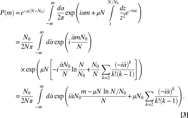This result is in accord with the Lea–Coulson scaling ansatz (2) that the N dependence of is captured by the variable

where it is easy to show that is the mean of m to lowest order in μ.

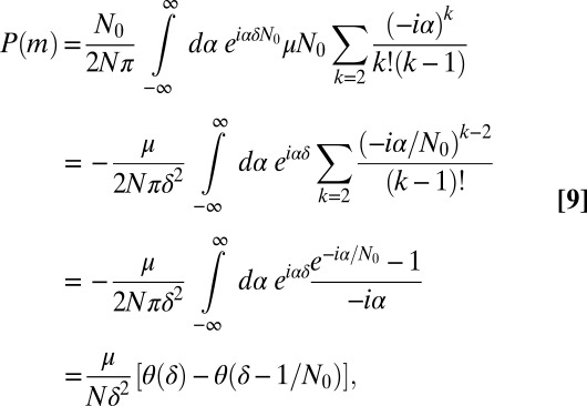
For small μ, there is an inner region where and an outer region where . In the inner region, we rescale and note that we can approximate the sum by its large argument limit:

where is the Euler–Mascheroni constant and Si and Ci are the sine and cosine integrals, respectively:

Using , as , we have

Thus,

This is nothing other than the Landau distribution:

The asymptotic behavior of is

as expected. Notice that this inner formula is independent of . This is because small clones originate near the end of the process, and so are independent of the initial conditions.

Finally, for , which means , we can expand Eq. 3 in μ and find the outer solution:

which cuts off the tail at .

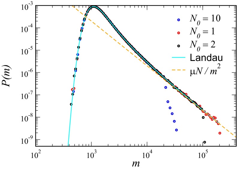
To check the validity of this result, we have directly simulated the sum in Eq. 2. The results are shown in Fig. 1, demonstrating the direct relevance of the Landau distribution as well as the sharp cutoff at .

Fig. 1.

P (m) for the original LD model from a simulation of realizations of the stochastic process in Eq. 2, together with the analytical Landau formula, for ; ; and , 2, and 10.

Stochastic LD Model: Outer Solution

An obvious refinement of the original LD model is to allow for the fact that birth events, for both the sensitive and mutant subpopulations, are also stochastic (20). Again, we assume that development of resistance is irreversible and mutants grow with no fitness disadvantage compared with wild-type (WT). As we shall see, the question of conditioning becomes crucial here, an issue that obviously does not arise in the quasideterministic original model, or in the Lea–Coulson (2) variant, where the WT grows deterministically. We start by conditioning on the total population, N, which matches most closely the quasideterministic earlier formulations. We will later see that conditioning on time (20, 21) yields very different answers in general.

The system, conditioned on N, is fully described by the master equation governing the probability of having m mutants among the N total members of the population, [i.e., that has undergone birth events (22)]:

where and . As before, μ is the mutation rate. The probability that there are no mutants is clearly

As in the original model, things are tremendously simplified if , and we work to linear order in μ. Then, the master equation takes the form

The last two terms are just birth without mutation, and the first term reflects the uniform rate of mutant creation, which arises from using the fact that , whereas is for all . The solution of this recursion relation can be seen to be

This is particularly simple for , where for , so that the power-law tail is sharply cut off past . In general, for large N,

and we again have a monotonic distribution, now with a smooth cutoff of the power-law tail as m approaches N. It is important to note that the presence of the power-law tail implies that all moments of the distribution are dominated by rare early birth, large m events, and thus are extremely difficult to measure in practice and strongly dependent on the initial conditions. As in the original model, this first order in μ solution breaks down for large enough N, such that is not small. Nonetheless, it is always valid (for small μ) for , which does, in fact, arise from early birth events that are always rare and so are treatable to linear order in μ. The vanishing of for is an immediate consequence of the fixed N ensemble in which we are working. In the fixed time ensemble, the nature of the outer behavior is exponential, because there is no limit to the total population at any fixed time. We next turn to the problem of general for m ≪ N, i.e., in the inner region.

Stochastic Model: Inner Solution

To derive the inner solution valid for large N and small μ (but with no constraint on ), we have to allow for terms in the distribution that are of arbitrary order in μ. However, to each order, we just need to keep the leading order in N. It is easy to see that terms of order have leading order dependence . If we denote the coefficient of this term in as , we find on substitution into the master equation (Eq. 12):

To derive this result, we used the fact that the coefficient of the term highest order in N (i.e., the term proportional to ) automatically vanishes, and the resultant equation emerges from the requirement that the coefficient of the order term vanishes as well. This equation is supplemented with for (because only the no-mutant sector is populated if ) and with , which follows from Eq. 11.

To solve this equation, we use a transform method. We multiply Eq. 15 by and sum from , and we denote the resulting function as . The distribution we want will be found from F via setting and identifying as the coefficient of in F. Proceeding, we obtain

We can convert this to a homogeneous equation, writing , so that

This homogeneous equation can be solved by the method of characteristics. We write and choose , whose solution is

where α labels the characteristic. Then, the equation for is the ordinary differential equation:

Solving with the boundary condition yields

Finally, we restore the original functional dependence on x and y using (from Eq. 18) to obtain

This result was originally derived by Lea–Coulson (2), but for the model where the WT population has deterministic growth dynamics. Note that the singular behavior at is ultimately responsible for the behavior at large m. Explicitly, for small :

which is, of course, the lowest order solution away from the cutoff region. It should be noted that our scaling solution cannot be used to determine the exact answers to higher than linear order in μ, however, because we have dropped higher order terms in μ, terms that do not scale as y.

As already mentioned, we can recover by extracting the coefficient of the term in an expansion about . This can be accomplished by contour integration in a small circle around the origin:

The integrand has a branch cut along the positive x axis starting at , associated with the aforementioned singular behavior. We can thus transform the contour integral into an integral of the discontinuity along the branch cut:

A similar expression based on the Lea–Coulson result appears in a paper by Kepler and Oprea (10).

If we further specialize to the case of large y, large m (because the scale of m is set by y), the integral is dominated by the region near . We thus write and denote , giving

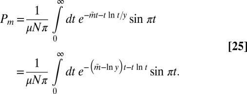This is just the Landau distribution, and our final answer is . Amazingly, this is exactly the same result [aside from a small shift in m of ] as we found for the original LD model. Note that this inner solution does not depend on , as we have come to expect. This lack of dependence of the inner solution on explains why the Lea–Coulson model, which ignores the stochasticity of the WT, produces the same large N distribution in the inner region as the fully stochastic model. Similarly, this is why the distribution agrees with that provided by Mandelbrot (18), who also used deterministic dynamics for the WT population. Because here there is no dependence, the effect of stochasticity can be made arbitrarily weak by taking large, and the models then coincide.

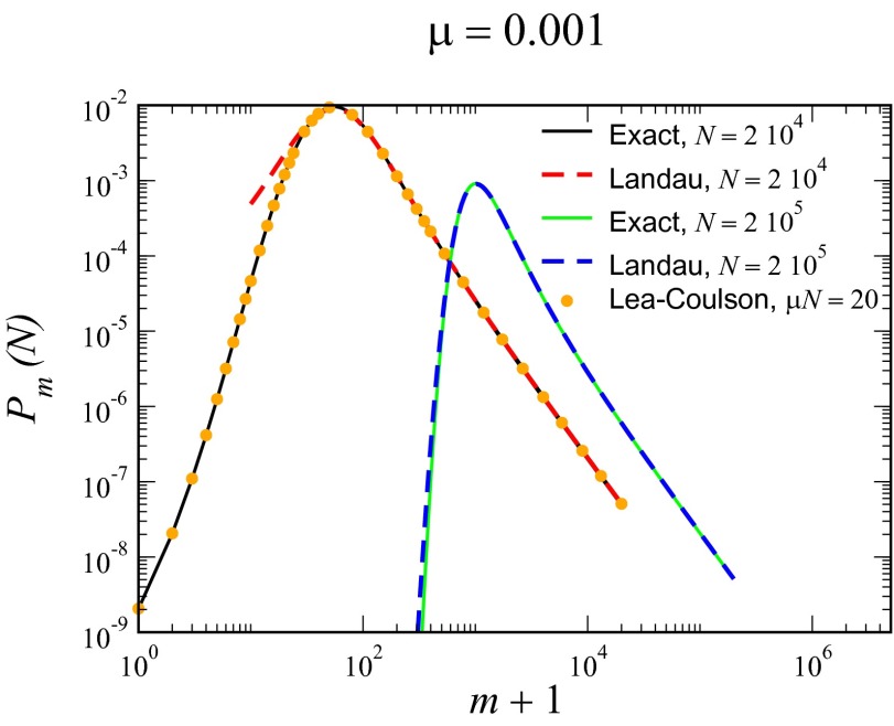
In Fig. 2, we compare this solution with an exact numerical calculation of the master equation with , with the latter not assuming anything regarding . The agreement is essentially perfect for the case but deviates for small μ from the exact answer when is reduced by an order of magnitude. The Lea–Coulson distribution, however, still works perfectly. Both approximations work all the way out to N, because the cutoff is sharp for . 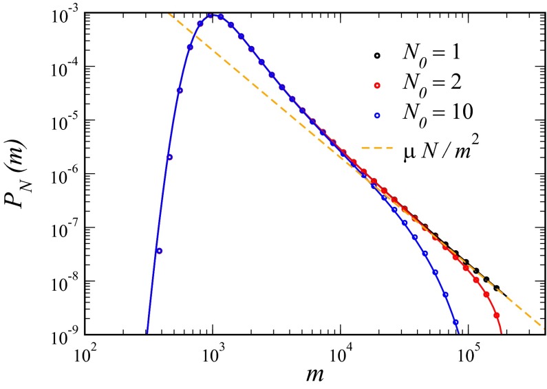Finally, in Fig. 3, we multiply this inner solution by the appropriate outer solution to create a composite solution valid for all values of m. This restores the dependence and shows how the Landau distribution is modified for .

Fig. 2.

Comparison of exact integration of the master equation (solid lines) vs. the Landau approximation (dashed lines) and the distribution represented by the Lea–Coulson generating function in Eq. 21 (dots) for , and , and .

Fig. 3.

Comparison of exact integration of the master equation (dots) vs. the Landau approximation (solid lines) with the appropriate factor for ; ; and , 2, and 10. Also shown is the asymptotic behavior.

Discussion

We have seen that in the fixed N ensemble for large N, small μ, the distribution can be divided into two regions, one an -independent inner region, where the Lea–Coulson generating function obtains, and the other an outer region, where is important and determines how the distribution is cut off. The Lea–Coulson distribution interpolates between two simple limiting behaviors: the monotonic decrease for small and the Landau distribution with its sharp rise at small m to a peak followed by a slow decay for large . In the first case, the most likely value of m is, of course, , whereas in the second, the mode is at . This is to be compared with the first moment of m, namely, , which we see larger by approximately . For a not untypical set of parameters, say , , the mode is at approximately , whereas the mean is ∼184. This reiterates how uninformative the mean is as a characterization of the distribution. Similar statements hold for the variance, and using these to estimate parameters of the evolution process by comparison with data is essentially impossible. This is a direct consequence of the (cutoff) power-law nature of the distribution, which is the underlying mechanism of the LD fluctuation experiment. The convergence to the α-stable Landau distribution at large is another consequence of this. As already mentioned, only one previous work (18) appears to have noticed this fundamental property of this process and that aspect of this work seems to have been completely ignored.

In this paper, we have focused on the original model with deterministic growth as well as the stochastic variation, where birth events occur probabilistically. In extensions to be discussed elsewhere, we show that the results presented here can be generalized to include differential fitness effects as well as effects of death. For completeness, we note that in each of those cases, the distribution in the large limit is a one-sided Lévy α-stable distribution, whose asymptotic power-law is determined solely by the fitness difference of the two subpopulations. The extension of the Lea–Coulson generating function to the differential fitness case is known (18), and it is again the inner solution to the fixed N stochastic problem. No similar results exist, however, for the case in which death is included.

It should be pointed out that the stochastic LD model is exactly solvable, and a formal but not very tractable explicit expression for the probability distribution has appeared previously (22). This was shown to reproduce the Lea–Coulson generating function in the inner region. The outer region was not analyzed. More crucially, the connection to power-law tails and, in particular, the Landau distribution seems not to have been appreciated in this work. This exact solution also applies only for equal birth rates and in the absence of death; thus, our approximate technique is more informative in the general case. It also should be noted that the analytical exact solution is, as a numerical tool, less effective than a direct solution of the master equation, because the number of operations is comparable and the exact solution involves terms of both signs, so that round off becomes an issue.

For the general case, Antal and Krapivsky (AK) (21) have recently derived a rather complex set of formulae embodying the solution for the generating function of the probability distribution in the fixed time ensemble, generalizing the results of Bartlett (20) for the neutral pure birth stochastic model. Bartlett succeeded in recovering the Lea–Coulson distribution in the limit of large , because the WT dynamics become deterministic there and the two ensembles coincide. To appreciate the problem, we first discuss the results of the time ensemble, working from the AK solution for the neutral pure birth model. The generating function of AK for , which is called , where y stands for WT and x for mutants, satisfies

where B is the generating function for the pure mutant growth problem, starting from a single mutant, which is given by

and , . The solution for A is given by

which can be seen, using the definition of z, to satisfy Eq. 26. The constant C is determined by the condition that , so that

The generating function for the mutants, independent of the number of WT cells, is given by . It is also convenient to work in terms of , the expected total population size, rather than t:

We thus obtain

We see immediately that the singularity at has been shifted to , so that the asymptotic decay of is exponential, and there is again a crossover from the inner region when .

The limit we wish to consider is the large , small μ limit: . In the inner region, we can drop the term, and we have

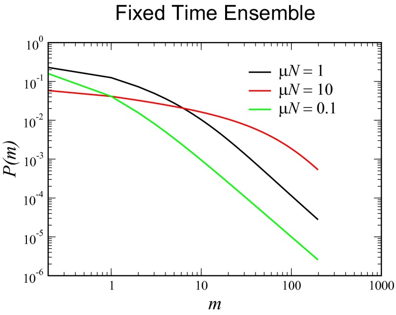
so that, again, is the relevant control parameter. However, this is not the Lea–Coulson generating function. In particular, , so that it does not decay exponentially with as in the fixed N ensemble. The reason for this is the presence of anomalous members of the fixed time ensemble with small total population sizes. Plotting the distribution that arises from this solution for various values of (Fig. 4), we see that there is no peak, ostensibly for the same reason.

Fig. 4.

Distribution for the fixed time ensemble resulting from Eq. 32 for , , and . Notice that in all cases, the distribution is monotonic decreasing and not at all like the Lea–Coulson result with its Landau limit at large .

Thus, going to the time ensemble makes a huge difference and, in fact, is not the relevant ensemble for application to cases where one measures N, for example, by determining the tumor size. We can recover relevant results if we additionally condition on N, that is, pick only those members of the statistical ensemble that have exactly individuals. This is gotten by looking at the coefficient of in A. We can do this analytically, because A is of the form , where :

Thus, the normalized generating function for the subensemble is explicitly

where is the normalization factor, chosen so that . Now, in the limit ,

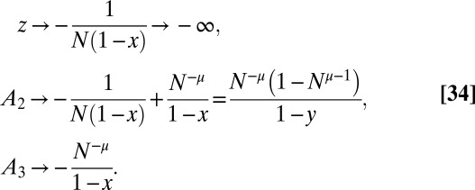Thus,

Given this, we now need to calculate the leading N behavior of . For fixed y, large N, , and

and

Collecting all the pieces, we arrive at the result that in this limit is equal to

This is just the Lea–Coulson result, including the term; thus, it also contains the small and Landau limits discussed above. Of course, the true fixed N ensemble contains contributions from different elapsed times, but this has no impact, because conditioning on N forces the time to be close to the nominal time (although conditioning on time does not force N to be close to its mean value). The small variation in these times clearly does not change the distribution, as can be shown explicitly.

Methods

Here, we present more information regarding the generation of the curves presented in the figures. The data for the original LD model was obtained for each realization by picking k from a Poisson distribution with mean and then summing k independent identically distributed random variables drawn from a distribution running from to . The individual sums were then logarithmically binned to generate the histogram.

The Landau distribution, , was computed for via the integral in Eq. 25. For , the form in Eq. 6 was used, where the region of integration was restricted to by symmetry, and the contour was then deformed to the steepest descent contour, extending from the critical point on the negative α axis off into the complex plane (23).

The data for the stochastic birth model were obtained via a direct solution of the master equation, Eq. 10. The data for the Lea–Coulson distribution came from a Taylor expansion of the generating function obtained from the symbolic algebra program Maple (Maplesoft). The data for the AK distribution came from a Maple-generated Taylor expansion of the corresponding generating function as well.

References

- 1.Luria SE, Delbrück M. Mutation of bacteria from virus sensitivity to virus resistance. Genetics. 1943;28(6):491–511. doi: 10.1093/genetics/28.6.491. [DOI] [PMC free article] [PubMed] [Google Scholar]
- 2.Lea DE, Coulson CA. The distribution of the numbers of mutants in bacterial populations. J Genet. 1949;49(3):264–285. doi: 10.1007/BF02986080. [DOI] [PubMed] [Google Scholar]
- 3.Lenski RE, Slatkin M, Ayala FJ. Mutation and selection in bacterial populations: Alternatives to the hypothesis of directed mutation. Proc Natl Acad Sci USA. 1989;86(8):2775–2778. doi: 10.1073/pnas.86.8.2775. [DOI] [PMC free article] [PubMed] [Google Scholar]
- 4.Coldman AJ, Goldie JH. A stochastic model for the origin and treatment of tumors containing drug-resistant cells. Bull Math Biol. 1986;48(3-4):279–292. doi: 10.1007/BF02459682. [DOI] [PubMed] [Google Scholar]
- 5.Moolgavkar SH. Carcinogenesis modeling: From molecular biology to epidemiology. Annu Rev Public Health. 1986;7(1):151–169. doi: 10.1146/annurev.pu.07.050186.001055. [DOI] [PubMed] [Google Scholar]
- 6.Komarova N. Stochastic modeling of drug resistance in cancer. J Theor Biol. 2006;239(3):351–366. doi: 10.1016/j.jtbi.2005.08.003. [DOI] [PubMed] [Google Scholar]
- 7.Tomasetti C, Levy D. An elementary approach to modeling drug resistance in cancer. Math Biosci Eng. 2010;7(4):905–918. doi: 10.3934/mbe.2010.7.905. [DOI] [PMC free article] [PubMed] [Google Scholar]
- 8.Diaz LA, Jr, et al. The molecular evolution of acquired resistance to targeted EGFR blockade in colorectal cancers. Nature. 2012;486(7404):537–540. doi: 10.1038/nature11219. [DOI] [PMC free article] [PubMed] [Google Scholar]
- 9.Clayton E, et al. A single type of progenitor cell maintains normal epidermis. Nature. 2007;446(7132):185–189. doi: 10.1038/nature05574. [DOI] [PubMed] [Google Scholar]
- 10.Kepler TB, Oprea M. Improved inference of mutation rates: I. An integral representation for the Luria-Delbrück distribution. Theor Popul Biol. 2001;59(1):41–48. doi: 10.1006/tpbi.2000.1498. [DOI] [PubMed] [Google Scholar]
- 11.Gerrish P. A simple formula for obtaining markedly improved mutation rate estimates. Genetics. 2008;180(3):1773–1778. doi: 10.1534/genetics.108.091777. [DOI] [PMC free article] [PubMed] [Google Scholar]
- 12.Dewanji A, Luebeck EG, Moolgavkar SH. A generalized Luria-Delbrück model. Math Biosci. 2005;197(2):140–152. doi: 10.1016/j.mbs.2005.07.003. [DOI] [PubMed] [Google Scholar]
- 13.Iwasa Y, Nowak MA, Michor F. Evolution of resistance during clonal expansion. Genetics. 2006;172(4):2557–2566. doi: 10.1534/genetics.105.049791. [DOI] [PMC free article] [PubMed] [Google Scholar]
- 14.Zheng Q. Progress of a half century in the study of the Luria-Delbrück distribution. Math Biosci. 1999;162(1-2):1–32. doi: 10.1016/s0025-5564(99)00045-0. [DOI] [PubMed] [Google Scholar]
- 15.Kashdan E, Pareschi L. Mean field mutation dynamics and the continuous Luria-Delbrück distribution. Math Biosci. 2012;240(2):223–230. doi: 10.1016/j.mbs.2012.08.001. [DOI] [PubMed] [Google Scholar]
- 16.Gentle JE. Random-Number Generation and Monte Carlo Methods. NY: Springer; 2003. p. 196. [Google Scholar]
- 17.Landau L. On the energy loss of fast particles by ionization. J Phys (USSR) 1944;8:201–205. [Google Scholar]
- 18.Mandelbrot B. A population birth-and-mutation process!: Explicit distributions for the number of mutants in an old culture of bacteria. J Appl Probab. 1974;11(3):437–444. [Google Scholar]
- 19.Gnedenko BV, Kolmogorov AN. Limit Distributions for Sums of Independent Random Variables. Reading, MA: Addison Wesley; 1954. [Google Scholar]
- 20.Bartlett MS. An Introduction to Stochastic Processes. UK: Cambridge Univ Press; 1955. [Google Scholar]
- 21.Antal T, Krapivsky PL. Exact solution of a two-type branching process: Models of tumor progression. J Stat Mech. 2011;2011(8):P08018. [Google Scholar]
- 22.Angerer WP. An explicit representation of the Luria-Delbrück distribution. J Math Biol. 2001;42(2):145–174. doi: 10.1007/s002850000053. [DOI] [PubMed] [Google Scholar]
-
23.Börsch-Supan W. On the evaluation of the function
for real values of λ. Journal of Research of the National Bureau of Standards B: Mathematics and Mathematical Physics. 1961;65B(4):245–250. [Google Scholar]